Phase behavior and structure of model colloid-polymer mixtures confined between two parallel planar walls

Abstract

Using Gibbs ensemble Monte Carlo simulations and density functional theory we investigate the fluid-fluid demixing transition in inhomogeneous colloid-polymer mixtures confined between two parallel plates with separation distances between one and ten colloid diameters covering the complete range from quasi two-dimensional to bulk-like behavior. We use the Asakura-Oosawa-Vrij model in which colloid-colloid and colloid-polymer interactions are hard-sphere like, whilst the pair potential between polymers vanishes. Two different types of confinement induced by a pair of parallel walls are considered, namely either through two hard walls or through two semi-permeable walls that repel colloids but allow polymers to freely penetrate. For hard (semi-permeable) walls we find that the capillary binodal is shifted towards higher (lower) polymer fugacities and lower (higher) colloid fugacities as compared to the bulk binodal; this implies capillary condensation (evaporation) of the colloidal liquid phase in the slit. A macroscopic treatment is provided by a novel symmetric Kelvin equation for general binary mixtures, based on the proximity in chemical potentials of statepoints at capillary coexistence and the reference bulk coexistence. Results for capillary binodals compare well with those obtained from the classic version of the Kelvin equation due to Evans and Marini Bettolo Marconi [J. Chem. Phys. 86, 7138 (1987)], and are quantitatively accurate away from the fluid-fluid critical point, even at small wall separations. However, the significant shift of the critical polymer fugacity towards higher values upon increasing confinement, as found in simulations, is not reproduced. For hard walls the density profiles of polymers and colloids inside the slit display oscillations due to packing effects for all statepoints. For semi-permeable walls either similar structuring or flat profiles are found, depending on the statepoint considered.

I Introduction

Capillary effects that are induced by the confinement of a system are crucial to a variety of phenomena. An everyday example is the capillary rise, against gravity, of the meniscus of a free gas-liquid interface at the wall of a container that encompasses the fluid. The contact angle at which the gas-liquid interface hits the wall is described by Young’s equation J. S. Rowlinson and B. Widom (2002), $\gamma_{\text{lg}}\cos\theta=\gamma_{\text{wg}}-\gamma_{\text{wl}}$, where the relevant interfacial tensions are those between the coexisting liquid and gas phase, $\gamma_{\text{lg}}$, the wall and the gas phase, $\gamma_{\text{wg}}$, and the wall and the liquid phase, $\gamma_{\text{wl}}$. When the contact angle is finite, $0<\theta<\pi$, the liquid phase partially wets the wall; for $\theta=0$ a macroscopic layer of liquid grows between the wall and the gas phase far away from the wall, hence the liquid completely wets the wall; for $\theta=\pi$ a correspondingly reversed situation occurs: a macroscopic layer of gas grows between the wall and the liquid phase far away from the wall, hence the wall is completely “wet” by the gas phase and drying occurs. All these phenomena are driven by the influence of a single wall on the fluid.

Different, but related effects occur under confinement of fluids in pores, e.g. between two parallel planar walls. The phase diagram of such a confined system can differ significantly from that in bulk Gelb et al. (1999); R. Evans (1990). Depending on the nature of the interactions between fluid particles and the walls, the bulk gas with chemical potential $\mu<\mu_{\text{sat}}$, where $\mu_{\text{sat}}$ is the value at saturation, can condense inside the pore and form a dense confined liquid phase. This capillary phase transition is accompanied by a jump in the adsorption isotherm at a given value of $\mu<\mu_{\text{sat}}$. Confinement may lead to stabilization of a phase that is unstable (or at least metastable) in bulk for a given statepoint. As opposed to capillary condensation the opposite effect, referred to as capillary evaporation, is also feasible: A fluid with chemical potential $\mu>\mu_{\text{sat}}$ forms a liquid in bulk, but evaporates inside the capillary. A simple, yet powerful, way to quantitatively describe capillary phase transitions is based on the Kelvin equation, derived from a macroscopic treatment of the thermodynamics of the inhomogeneous system. For capillaries with planar slit-like geometries R. Evans and U. Marini Bettolo Marconi (1987), it predicts that liquid-gas coexistence inside the slit will occur at $\mu=\mu_{\text{sat}}+\gamma_{\text{lg}}\cos(\theta)/h$, where $h$ is the separation distance between the two walls. Hence, contact angles $0\leq\theta<\pi/2$ correspond to capillary condensation, while $\pi/2<\theta\leq\pi$ corresponds to capillary evaporation.

In this work we investigate capillary phenomena occurring on a mesoscopic scale using a simple model for a mixture of sterically-stabilized colloidal particles and non-adsorbing polymer coils confined between two parallel planar walls. Using colloids as model systems offers advantages over molecular substances due to easy experimental access to the relevant length and time scales, and the possiblilty of using real space techniques like confocal microscopy. Our work is intended to stimulate such investigations in order to gain further insights into capillary phenomena. The topology of the bulk phase diagram of colloid-polymer mixtures depends on the polymer size (as compared to the size of the colloids) and the polymer concentration. At sufficiently high polymer concentration and for sufficiently large polymer, the bulk system demixes into a colloidal liquid phase that is rich in colloids (and dilute in polymers), and a colloidal gas phase that is dilute in colloids (and rich in polymers) Meijer and Frenkel (1991, 1994); Ilett et al. (1994); M. Dijkstra et al. (1999); M. Dijkstra (2001). This phenomenology is similar to gas-liquid coexistence in simple fluids with the polymer fugacity $z_{\text{p}}$ playing the role of inverse temperature, and hence governing the strength of interparticle attractions. However the phase separation in colloid-polymer mixtures is purely entropy-driven, due to an effective depletion interaction between the colloidal particles, that is mediated by the polymer W. C. K. Poon (2002); Tuinier et al. (2003). A similar mechanism induces an effective depletion interaction between a colloidal particle and a planar hard wall J. M. Brader et al. (2001). For a review on the properties of colloid-polymer mixtures in contact with a hard wall, we refer the reader to Brader et al. J. M. Brader et al. (2003). Recently the wall-fluid interfacial tensions D. G. A. L. Aarts et al. (2004); P. P. F. Wessels et al. (2004a); Fortini et al. (2005) and the contact angle of the free interface and a hard wall P. P. F. Wessels et al. (2004b), and the gas-liquid interfacial tension R. L. C. Vink and J. Horbach (2004a, b) have been studied theoretically and with computer simulations. Moreover complete wetting of the colloidal liquid phase at a hard wall is found, close to the critical point, in both simulation M. Dijkstra and R. van Roij (2002); Dijkstra and van Roij (2005); Dijkstra et al. (2005) and theory J. M. Brader et al. (2003, 2002). Complete wetting of the colloidal liquid is also observed in experimental realizations of colloid-polymer mixtures in contact with glass substrates D. G. A. L. Aarts et al. (2003); D. G. A. L. Aarts and H. N. W. Lekkerker (2004) or glass substrates that possess the same coating with an organophilic group as the colloidal particles do W. K. Wijting et al. (2003a). On the other hand, experiments W. K. Wijting et al. (2003b) with polymer-grafted substrates (of the same chemical nature as the dissolved polymers) showed that the contact angle is larger than $\pi/2$. Although the structure of the polymer coating was not studied in detail, Wijting et al. W. K. Wijting et al. (2003b) expect the polymers to form a fluffy layer with a distribution of loops and tails. Such a layer is known to diminish the depletion interaction between colloidal particles and the substrate Jenkins and Snowden (1996). Wessels et al. P. P. F. Wessels et al. (2004a) modeled this type of substrate using a semi-permeable wall, that is completely penetrable to the polymers but act like a hard wall on the colloids. Using DFT they predict complete drying. More recently the behavior of the mixtures in contact with porous walls was investigated, and both wetting of the surface and drying into the porous matrix depending on the precise path in the phase diagram were found Wessels et al. (2005). Porous walls are wet by the liquid phase, with a transition from partial to complete wetting at a polymer fugacity $z_{\text{p}}$ almost independent on the porosity of the wall.

Although much research has been devoted to the understanding of the behavior of the mixture in contact with a single wall, few studies have been reported on the effect of confinement on the phase behavior of the mixture. Computer simulations and theory were used to study porous matrices. When impenetrable to both components they were found to induce capillary condensation, whereas matrices penetrable to the polymers, but not to the colloids, induce capillary evaporation M. Schmidt et al. (2002a); Wessels et al. (2003). Furthermore laser induced confinement I. O. Götze et al. (2003) was found to induce capillary condensation. The only experimental result on capillary condensation that we are aware of is that by Aarts et al. D. G. A. L. Aarts and H. N. W. Lekkerker (2004). These authors found capillary condensation for colloid-polymer mixtures confined in a wedge formed by a glass bead placed on a glass substrate.

The aim of the present paper is to determine the phase behavior and the structure of colloid-polymer mixtures confined between two parallel planar walls for a complete range of wall separation distances. We focus on the fluid part of the phase diagram, and present results for hard walls and semi-permeable walls, obtained from computer simulations and density functional theory. A preliminary account of this work was given in Refs. M. Schmidt et al. (2003, 2004). Here we supply all relevant details of the simulation method. We also investigate the structure of the mixtures inside the pore, and derive and test a generalized Kelvin equation for binary mixtures confined in slit-like pores and compare its predictions with our simulation results.

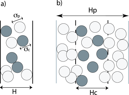
Figure 1: (a) Illustration of the AOV model of hard sphere colloids (gray circles) of diameter $\sigma_{\text{c}}$ and ideal polymers (transparent circles) of diameter $\sigma_{\text{p}}$ confined between parallel hard walls of area $A$ and separation distance $H$. Colloids behave as hard spheres, polymers cannot penetrate colloids, and polymers may freely overlap. The walls are impenetrable to both components. The $z$-axis is perpendicular to both walls, and the origin is located in the middle of the slit. (b) Same as in (a) but for walls that are penetrable for polymers and impenetrable for colloids (semi-permeable walls) of area $A$ and separation distance $H_{\text{c}}$. Polymers are confined between parallel hard walls (continuous line) with separation distance $H_{\text{p}}$. This is a model for substrates at distance $H_{\text{p}}$ coated with a polymer brush (not shown) of thickness $(H_{\text{p}}-H_{\text{c}})/2$; the free distance between both polymer brushes is $H_{\text{c}}$. Solute polymers (open spheres) are able to penetrate the brush (dashed lines) but not the substrate; the brush acts like a hard wall to the colloids.

II Model

Consider a binary mixture of $N_{\text{c}}$ hard spheres of diameter $\sigma_{\text{c}}$ representing the colloidal particles and $N_{\text{p}}$ non-interacting spheres of diameter $\sigma_{\text{p}}$ representing the (ideal) polymers in a volume $V$ at temperature $T$. This is a simple model for a colloid-polymer mixture as the interaction between sterically-stabilized colloids can be made such that it resembles closely that of hard spheres, and a dilute solution of polymers in a $\theta$-solvent is weakly interacting. Colloids and polymers interact via a hard-sphere-like potential, as the polymers are excluded from a centre-of-mass distance $(\sigma_{\text{c}}+\sigma_{\text{p}})/2$ from the colloid, where $\sigma_{\text{p}}=2R_{g}$, and $R_{g}$ is the radius of gyration of the polymer coils. We treat the solvent as an inert continuum. This so-called Asakura-Oosawa-Vrij (AOV) model S. Asakura and F. Oosawa (1954); Asakura and Oosawa (1958); A. Vrij (1976) is defined by the pair potentials

$$v_{\text{cc}}(R_{ij})=\left\{\begin{array}[]{ll}\infty&\textrm{ if $R_{ij}<\sigma_{\text{c}}$ }\\ 0&\textrm{otherwise},\end{array}\right.$$ (1)

where $R_{ij}=|\vec{R}_{i}-\vec{R}_{j}|$ is the distance between two colloidal particles, with $\vec{R}_{i}$ the position of the centre-of-mass of colloid $i$,

$$v_{\text{pp}}(r_{ij})=0,$$ (2)

where $r_{ij}=|\vec{r_{i}}-\vec{r_{j}}|$ is the distance between two polymers, with $\vec{r_{i}}$ the position of the centre-of-mass of polymer $i$ and

$$v_{\text{cp}}(|\vec{R}_{i}-\vec{r}_{j}|)=\left\{\begin{array}[]{ll}\infty&\textrm{ if $|\vec{R}_{i}-\vec{r}_{j}|<(\sigma_{\text{c}}+\sigma_{\text{p}})/2$ }\\ 0&\textrm{ otherwise,}\end{array}\right.$$ (3)

where $|\vec{R}_{i}-\vec{r}_{j}|$ is the distance between colloid $i$ and polymer $j$.

The size ratio $q=\sigma_{\text{p}}/\sigma_{\text{c}}$ is a geometric parameter that controls the range of the effective depletion interaction between the colloids. We denote the packing fraction by $\eta_{k}=(\pi\sigma_{k}^{3}N_{k})/(6V)$, with $k=\text{c, p}$ for colloids and polymers, respectively. As alternatives to $\eta_{\text{p}}$, we use as a thermodynamic variable the colloidal fugacity $z_{\text{c}}$, or the polymer reservoir packing fraction $\eta_{\text{p}}^{\text{r}}$ that satisfies the (ideal gas) relation

$$\eta_{\text{p}}^{\text{r}}=\frac{\pi}{6}\sigma_{\text{p}}^{3}z_{\text{p}}.$$ (4)

The hard walls are modeled such that neither polymers nor colloids can penetrate the walls. The wall-particle potential acting on species $k=\text{c, p}$ is

$$v_{\text{w}k}(z)=\left\{\begin{array}[]{ll}0&\textrm{if $-(H-\sigma_{k})/2<z<(H-\sigma_{k})/2$ }\\ \infty&\textrm{otherwise,}\end{array}\right.$$ (5)

where $z$ is the coordinate normal to the walls, and $H$ is the wall separation distance. We define the volume of the system as $V=AH$, where $A$ is the (lateral) area of the confining walls. Fig. 1(a) shows an illustration of the model.

Semi-permeable walls are defined by the external potential

$$v_{\text{w}k}(z)=\left\{\begin{array}[]{ll}0&\textrm{if $-(H_{k}-\sigma_{k})/2<z<(H_{k}-\sigma_{k})/2$ }\\ \infty&\textrm{otherwise,}\end{array}\right.$$ (6)

where $H_{\text{c}}$ is the wall separation distance that the colloids experience, while $H_{\text{p}}$ is the wall separation distance that the polymers feel; the latter can be interpreted as the distance between substrate walls. We define the volume as $V=AH_{\text{c}}$. Fig. 1(b) shows an illustration of this model. Any choice of $H_{\text{p}}>H_{\text{c}}+2\sigma_{\text{p}}$ leads to decoupling of the (inner) colloid and (outer) polymer wall, since the ideal gas of polymers cannot mediate correlations from the substrate to the interior of the system.

III Simulation method

We perform Gibbs Ensemble Monte Carlo (GEMC) simulations to determine the phase behavior of the AOV model in bulk and confined between two parallel planar walls. The number of colloids $N_{\text{c}}$, the number of polymers $N_{\text{p}}$, and the volume $V$ are kept fixed and are divided into two separate subsystems a and b with volume $V^{\text{a}}$ and $V^{\text{b}}$, respectively, with the constraints that $V=V^{\text{a}}+V^{\text{b}}$ , $N_{\text{c}}=N_{\text{c}}^{\text{a}}+N_{\text{c}}^{\text{b}}$ and $N_{\text{p}}=N_{\text{p}}^{\text{a}}+N_{\text{p}}^{\text{b}}$. The two subsystems are allowed to exchange both particles and volume in order to satisfy the conditions for phase equilibrium, i.e., equality in both phases of the chemical potentials of the two species and of the pressure. The method can be applied to bulk as well as to confined systems A. Z. Panagiotopoulos (1987a, b), and will be described briefly below; for more details, we refer the reader to Ref. D. Frenkel and B. Smit (2002).

In more detail, the bulk equilibrium conditions between two coexisting phases require equal temperature $T$, equal chemical potential $\mu_{i}$ for each species $i$ ($i=\text{c, p}$ in our case) and equal pressure $P$. In our model, the temperature $T$ is irrelevant; because of the hard-core nature of the interaction potentials it acts only as a scaling factor setting the thermal energy scale. In the GEMC method, the two coexisting phases are simulated simultaneously in two separate (cubic) boxes with standard periodic boundary conditions. The acceptance probability for a trial move to displace a randomly selected particle is

$$\mathcal{P}=\text{min}\{1,\exp[-\beta(U_{\text{new}}-U_{\text{old}})]\},$$ (7)

where

$$\exp[-\beta(U_{\text{new}}-U_{\text{old}})]=\left\{\begin{array}[]{ll}1&\textrm{ if $\beta U_{\text{new}}=0$ }\\ 0&\textrm{ if $\beta U_{\text{new}}=\infty$ }\end{array}\right.$$ (8)

with $U_{\text{new}}$ and $U_{\text{old}}$ the energy of the new and old generated configuration, and $\beta=1/(k_{B}T)$ the inverse temperature with $k_{B}$ being the Boltzmann constant. Note that $U_{\text{old}}=0$ as configurations with $U_{\text{old}}=\infty$ are excluded by a vanishing Boltzmann factor (regardless of the temperature). Transfer of (single) particles between the two boxes is used to satisfy equal chemical potential for both species. We select at random which subsystem is the donor and which is the recipient as well as the species (colloid or polymer) of the particle transfer. Subsequently, a specific particle is randomly selected in the donor box and transferred to a random position in the recipient box with probability

$$\mathcal{P}=\text{min}\left\{1,\frac{N_{i}^{\text{a}}V^{\text{b}}}{(N_{i}^{\text{b}}+1)V^{\text{a}}}\exp[-\beta(U_{\text{new}}-U_{\text{old}})]\right\},$$ (9)

where $i=\text{c, p}$ is the species of the selected particle, $V^{\text{a}}$ is the volume of the donor box and $V^{\text{b}}$ is the volume of the recipient box.

In addition, volume changes of the boxes are used to satisfy the condition of equal pressure in both subsystems. We hence perform a random walk in $\ln(V_{a}/V_{b})$ with the acceptance probability

$$\mathcal{P}=\text{min}\left\{1,\mathcal{R}\exp[-\beta(U_{\text{new}}-U_{\text{old}})]\right\},$$ (10)

where

$$\mathcal{R}=\left(\frac{V^{\text{a}}_{\text{new}}}{V^{\text{a}}_{\text{old}}}\right)^{N_{\text{c}}^{\text{a}}+N_{\text{p}}^{\text{a}}+1}\left(\frac{V^{\text{b}}_{\text{new}}}{V^{\text{b}}_{\text{old}}}\right)^{N_{\text{c}}^{\text{b}}+N_{\text{p}}^{\text{b}}+1},$$ (11)

and with the condition that the total volume $V=V^{\text{a}}_{\text{old}}+V^{\text{b}}_{\text{old}}=V^{\text{a}}_{\text{new}}+V^{\text{b}}_{\text{new}}$ is constant , where the subscript old (new) marks quantities before (after) the trial displacement.

Phase equilibria in confined geometries, like e.g. inside slit pores as considered here, can be determined by either determining the adsorption isotherm in simulation or by employing the GEMC simulation method extended to a slit pore A. Z. Panagiotopoulos (1987b). In the first method, the pore is coupled to a reservoir of bulk fluid. The adsorption of the fluid inside the pore is then measured at constant temperature for different bulk densities of the reservoir, i.e. the chemical potentials of the various species are fixed. A jump in the adsorption isotherm corresponds to capillary condensation or evaporation in the slit pore. However, this method is inaccurate for determining phase coexistence due to hysteresis.

In order to determine the binodal lines, we hence employ the GEMC method adapted to a slit pore A. Z. Panagiotopoulos (1987b): Two separate simulation boxes are simulated, one containing the confined gas and one containing the confined liquid. Each box has periodic boundary conditions in both directions parallel to the walls. Capillary coexistence implies equality of temperature, chemical potentials for both species as well as equality of the wall-fluid interfacial tension. Fulfilling the first two conditions is performed similar to the procedure for determining bulk phase equilibria, i.e. using particle displacements with acceptance probability given by Eq. (7) and particle transfers with acceptance probability given by Eq. (9). We satisfy the third requirement of equal wall-fluid interfacial tension in both phases by exchanging wall area (and hence volume) between the two boxes, while fixing both the wall separation distance $H$ in each box as well as the total lateral area of both boxes $A^{\text{a}}+A^{\text{b}}=A$ is constant, with $A^{\text{a}}$ and $A^{\text{b}}$ the area of the subsystems a and b, respectively. A random walk in $\ln(A^{\text{a}}/A^{\text{b}})$ is then performed with an acceptance probability given by

$$\mathcal{P}=\text{min}\left\{1,\mathcal{R}\exp[-\beta(U_{\text{new}}-U_{\text{old}})]\right\},$$ (12)

with

$$\mathcal{R}=\left(\frac{A^{\text{a}}_{\text{new}}}{A^{\text{a}}_{\text{old}}}\right)^{N_{\text{c}}^{\text{a}}+N_{\text{p}}^{\text{a}}+1}\left(\frac{A^{\text{b}}_{\text{new}}}{A^{\text{b}}_{\text{old}}}\right)^{N_{\text{c}}^{\text{b}}+N_{\text{p}}^{\text{b}}+1}.$$ (13)

We determine the fugacities of the colloids and of the polymers by applying the GEMC version of the particle insertion method B. Smit and D. Frenkel (1989)

$$z_{k}^{\text{a,b}}=\left<\frac{V^{\text{a,b}}}{N^{\text{a,b}}_{k}+1}\exp[-\beta\Delta U]\right>^{-1}\,k=\text{c, p}$$ (14)

where $a,b$ label the two simulation boxes and $\Delta U$ is the energy defined by the acceptance rule of Eq. (9). We determine the densities of the two coexisting phases by sampling histograms of the probability density $P(\eta_{\text{c}},\eta_{\text{p}})$ to observe the packing fractions $\eta_{\text{p}}$ and $\eta_{\text{c}}$ for the polymers and colloids, respectively. The two maxima of $P(\eta_{\text{c}},\eta_{\text{p}})$ correspond to the coexisting packing fractions in the thermodynamic limit B. Smit and D. Frenkel (1989). Statistical uncertainties of the sampled quantities were determined by performing three or four independent sets of simulations. The standard deviation of the results from the simulation sets was used as the error estimate.

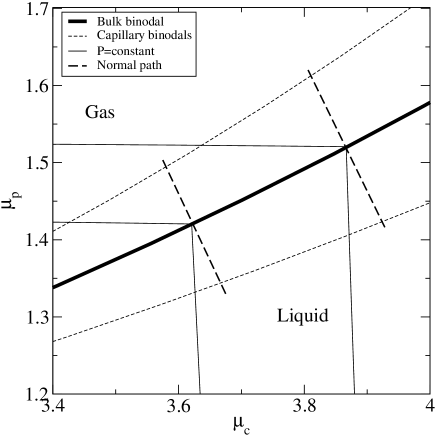
Figure 2: Phase diagram of the AOV model with size ratio $q=\sigma_{\text{p}}/\sigma_{\text{c}}=1$ as a function of the colloidal chemical potential $\mu_{\text{c}}$ and the polymer chemical potential $\mu_{\text{p}}$. The bulk binodal from free volume theory (thick continuous curve) is shown along with isobaric lines (thin continuous curves) for two bulk reference points. The thick dashed curves indicate the normal paths for the same reference points. The thin dashed curves are an illustration of the possible prediction of the Kelvin equation for the capillary binodals. For clarity we omitted the paths with constant polymer chemical potential.

IV Kelvin equation for binary mixtures

In this Section, we derive expressions for the shift in chemical potentials for the gas-liquid binodal of a binary mixture confined between parallel plates assuming knowledge of bulk quantities like the bulk coexisting densities, the chemical potentials at bulk coexistence, and the liquid-wall and gas-wall interfacial tensions, $\gamma_{\rm wl}$ and $\gamma_{\rm wg}$, respectively. Using a macroscopic picture we employ the grand potential of the mixture confined in a slit of two parallel walls with area $A$ and separation distance $h$ between the two walls

$$\Omega(\mu_{\rm c},\mu_{\rm p})=Ah\omega(\mu_{\rm c},\mu_{\rm p})+2A\gamma(\mu_{\rm c},\mu_{\rm p},h),$$ (15)

where $\mu_{\rm c}$ and $\mu_{\rm p}$ are the chemical potentials of colloids and polymers, respectively, $\omega$ is the bulk grand potential density (per unit volume), and $2\gamma$ is the interfacial tension of the mixture and the plates at distance $h$. For large $h$, we can approximate the latter quantity by twice the interfacial tension of the mixture in contact with a single wall, e.g., $2\gamma_{\rm w\alpha}(\mu_{\rm c},\mu_{\rm p})$, where $\alpha$=l,g are for the liquid and the gas phase, respectively. The aim is to predict the grand potential in the capillary given the knowledge of the thermodynamics of the bulk at coexistence, i.e. at a statepoint specified through the bulk values of the chemical potentials $\mu_{\rm c}^{\rm\ast}$ and $\mu_{\rm p}^{\rm\ast}$. Hence, we can reexpress the chemical potentials of both species for the confined fluid as $\mu_{\rm c}=\mu_{\rm c}^{\rm\ast}+\Delta\mu_{\rm c}$ and $\mu_{\rm p}=\mu_{\rm p}^{\rm\ast}+\Delta\mu_{\rm p}$. Quantities at coexistence carry a superscript $\alpha=\rm l,g$, where $\rm l,g$ indicate liquid and gas respectively.

The thermodynamic relations for the bulk densities of the colloids and polymers, $\rho_{c}$ and $\rho_{p}$, respectively, read

$$\rho_{\rm c}=-\left.\frac{\partial\omega}{\partial\mu_{\rm c}}\right|_{\mu_{\rm p}},\quad\rho_{\rm p}=-\left.\frac{\partial\omega}{\partial\mu_{\rm p}}\right|_{\mu_{\rm c}},$$ (16)

while the (excess) adsorption of the colloids and the polymers, $\Gamma_{c}$ and $\Gamma_{p}$, are given by

$$\Gamma_{\rm c}=\left.\frac{\partial\gamma_{\rm w\alpha}}{\partial\mu_{\rm c}}\right|_{\mu_{\rm p}},\quad\Gamma_{\rm p}=\left.\frac{\partial\gamma_{\rm w\alpha}}{\partial\mu_{\rm p}}\right|_{\mu_{\rm c}}.$$ (17)

Using Eqs. (16) and (17), we can perform a Taylor expansion of the right hand side of Eq. (15)

$$\frac{1}{Ah}\Omega(\mu_{\rm c},\mu_{\rm p})\approx \omega(\mu_{\rm c}^{\rm\ast},\mu_{\rm p}^{\rm\ast})-\rho_{\rm c}^{\alpha}\Delta\mu_{\rm c}-\rho_{\rm p}^{\alpha}\Delta\mu_{\rm p}$$ (18)

$$+\frac{2}{h}\Bigl{[}\gamma_{{\rm w}\alpha}+\Gamma_{\rm c}^{\alpha}\Delta\mu_{\rm c}+\Gamma_{\rm p}^{\alpha}\Delta\mu_{\rm p}\Bigr{]},$$

where the bulk densities, $\rho_{\rm c}^{\alpha}$ and $\rho_{\rm p}^{\alpha}$, and the (excess) adsorptions, $\Gamma_{c}^{\alpha}$ and $\Gamma_{\rm p}^{\alpha}$, are evaluated in one of the coexisting phases $\alpha=\rm l,g$ at the statepoint given by $\mu_{\rm c}^{\rm\ast}$ and $\mu_{\rm p}^{\rm\ast}$.

We next consider the capillary to be at phase coexistence, i.e. we might envisage two capillaries in contact with each other, one being filled with gas, the other being filled with liquid. Phase equilibrium between both capillaries implies equality of the chemical potential of each species and of the grand potential in both phases,

$$\Omega_{\rm g}(\mu_{\rm c},\mu_{\rm p})=\Omega_{\rm l}(\mu_{\rm c},\mu_{\rm p}),$$ (19)

where $\Omega_{\rm g}$ and $\Omega_{\rm l}$ is the grand potential of the gas and the liquid phase, respectively. Using the approximation (18) in (19) yields

$$\Bigl{(}\rho_{\rm c}^{\rm l}-\rho_{\rm c}^{\rm g}-\frac{2}{h}(\Gamma_{\rm c}^{\rm l}-\Gamma_{\rm c}^{\rm g})\Bigr{)}\Delta\mu_{\rm c}$$ (20)

$$+ \Bigl{(}\rho_{\rm p}^{\rm l}-\rho_{\rm p}^{\rm g}-\frac{2}{h}(\Gamma_{\rm p}^{\rm l}-\Gamma_{\rm p}^{\rm g})\Bigr{)}\Delta\mu_{\rm p}\quad$$

$$= \frac{2}{h}\Bigl{(}\gamma_{\rm wl}(\mu_{\rm c}^{\rm\ast},\mu_{\rm p}^{\rm\ast})-\gamma_{\rm wg}(\mu_{\rm c}^{\rm\ast},\mu_{\rm p}^{\rm\ast})\Bigr{)}.$$

In the limit $h$ is large compared with the microscopic lengths and that the adsorptions remain finite, we can neglect the terms proportional to $(\Gamma_{i}^{\rm l}-\Gamma_{i}^{\rm g})/h$. Hence, Eq. (20) simplifies to

$$\bigl{(}\rho_{\rm c}^{\rm l}-\rho_{\rm c}^{\rm g}\bigr{)}\Delta\mu_{\rm c}+\bigl{(}\rho_{\rm p}^{\rm l}-\rho_{\rm p}^{\rm g}\bigr{)}\Delta\mu_{\rm p}=\frac{2}{h}\Bigl{(}\gamma_{\rm wl}-\gamma_{\rm wg}\Bigr{)},$$ (21)

which constitutes a single equation for the two unknown shifts in the chemical potentials, $\Delta\mu_{\rm c}$ and $\Delta\mu_{\rm p}$. In order to obtain a closed system of equations one requires another assumption. We will present three different approaches in the following. Each approach can be viewed as a different choice of an “optimal” bulk reference state as illustrated in Fig. 2. A comparison with the numerical results will be presented in Sec. V.5.

IV.1 Constant Polymer Chemical Potential

The bulk reference state is chosen to be at the same polymer chemical potential. This requirement is similar to imposing the same temperature in a simple substance. The optimal bulk reference state with the same chemical potential of polymers leads to

$$\Delta\mu_{\rm p}=0.$$ (22)

Eqs. (21) and (22) readily yield a one-component Kelvin equation

$$\Delta\mu_{\rm c}=\frac{2}{h}\frac{\gamma_{\rm wl}-\gamma_{\rm wg}}{\rho_{\rm c}^{\rm l}-\rho_{\rm c}^{\rm g}}.$$ (23)

Clearly this result can be obtained with less labour by directly dealing with the effective one-component system of colloids interacting with a depletion potential, and rather serves as a illustration for the validity of the reasoning leading to Eq. (21).

IV.2 Constant Pressure

This reference state was used by Evans and Marini Bettolo Marconi in Ref. R. Evans and U. Marini Bettolo Marconi (1987). The bulk reference state is chosen to possess the same pressure. In order to derive a corresponding condition consider the (finite difference version of the) Gibbs-Duhem relation

$$(S/V)\Delta T-\Delta P+\rho_{\rm c}\Delta\mu_{\rm c}+\rho_{\rm p}\Delta\mu_{\rm p}=0,$$ (24)

where $S$ is the entropy. Clearly, for athermal systems $\Delta T=0$. We use (24) to compare the statepoint at capillary coexistence with the reference statepoint at bulk coexistence that possesses the same pressure, i.e. $\Delta P=0$, hence

$$\Delta\mu_{\rm p}=-\frac{\rho_{\rm c}^{\alpha}}{\rho_{\rm p}^{\alpha}}\Delta\mu_{\rm c},\quad\alpha=\rm g,l.$$ (25)

As shown in Fig. 2 the constant pressure paths (for which the Gibbs-Duhem relation is a good approximation close to the bulk binodal) have a discontinuity at bulk coexistence. To predict the capillary phase behavior for statepoints that lie on the gas side of the bulk gas-liquid binodal (hence to predict capillary condensation), the correct reference state is the coexisting gas phase, and we use (25) with $\alpha=\rm g$. Together with (21) we obtain the classic result for capillary condensation,

$$\Delta\mu_{\rm c} = \frac{2}{h}\frac{\gamma_{\rm wl}-\gamma_{\rm wg}}{\rho_{\rm c}^{\rm l}-(\rho_{\rm c}^{\rm g}/\rho_{\rm p}^{\rm g})\rho_{\rm p}^{\rm l}},$$

$$\Delta\mu_{\rm p} = \frac{2}{h}\frac{\gamma_{\rm wl}-\gamma_{\rm wg}}{\rho_{\rm p}^{\rm l}-(\rho_{\rm p}^{\rm g}/\rho_{\rm c}^{\rm g})\rho_{\rm c}^{\rm l}}.$$ (26)

Alternatively, predicting the capillary phase behavior for statepoints that lie on the liquid side of the bulk gas-liquid binodal (and to predict capillary evaporation), we choose the coexisting liquid phase as a reference. Eq. (25) with $\alpha=\rm l$ together with Eq. (21) leads to the following result for capillary evaporation

$$\Delta\mu_{\rm c} = -\frac{2}{h}\frac{\gamma_{\rm wl}-\gamma_{\rm wg}}{\rho_{\rm c}^{\rm g}-(\rho_{\rm c}^{\rm l}/\rho_{\rm p}^{\rm l})\rho_{\rm p}^{\rm g}},$$

$$\Delta\mu_{\rm p} = -\frac{2}{h}\frac{\gamma_{\rm wl}-\gamma_{\rm wg}}{\rho_{\rm p}^{\rm g}-(\rho_{\rm p}^{\rm l}/\rho_{\rm c}^{\rm l})\rho_{\rm c}^{\rm g}}.$$ (27)

The derivation presented here yields the same results as given in Ref. R. Evans and U. Marini Bettolo Marconi (1987), where a single capillary is considered in contact with a bulk reservoir. We note that this procedure leads to two different equations for the two phenomena of capillary condensation and evaporation.

IV.3 Normal Path Relation

As a third and novel alternative we choose the reference state such that the statepoint of interest lies on a path in the phase diagram that crosses the bulk liquid-gas binodal in perpendicular (or normal) direction in the plane of chemical potentials. This implies optimizing proximity in the $\mu_{c}-\mu_{p}$ plane between both statepoints.

The corresponding relation can readily be established starting from the relation of the slope of the bulk binodal to the difference in coexisting densities,

$$\left.\frac{d\mu_{\rm c}}{d\mu_{\rm p}}\right|_{\rm coex}=-\frac{\rho_{\rm p}^{\rm l}-\rho_{\rm p}^{\rm g}}{\rho_{\rm c}^{\rm l}-\rho_{\rm c}^{\rm g}}.$$ (28)

Hence a path normal to the bulk binodal is given by

$$\left.\frac{d\mu_{\rm c}}{d\mu_{\rm p}}\right|_{\rm normal}=\frac{\rho_{\rm c}^{\rm l}-\rho_{\rm c}^{\rm g}}{\rho_{\rm p}^{\rm l}-\rho_{\rm p}^{\rm g}},$$ (29)

from which we deduce the finite-difference version

$$\Delta\mu_{\rm p}=\frac{\rho_{\rm p}^{\rm l}-\rho_{\rm p}^{\rm g}}{\rho_{\rm c}^{\rm l}-\rho_{\rm c}^{\rm g}}\Delta\mu_{\rm c},$$ (30)

which, together with Eq. (21) yields

$$\Delta\mu_{\rm c} = \frac{2}{h}(\gamma_{\rm wl}-\gamma_{\rm wg})\frac{\rho_{\rm c}^{\rm l}-\rho_{\rm c}^{\rm g}}{(\rho_{\rm c}^{\rm l}-\rho_{\rm c}^{\rm g})^{2}+(\rho_{\rm p}^{\rm l}-\rho_{\rm p}^{\rm g})^{2}},$$

$$\Delta\mu_{\rm p} = \frac{2}{h}(\gamma_{\rm wl}-\gamma_{\rm wg})\frac{\rho_{\rm p}^{\rm l}-\rho_{\rm p}^{\rm g}}{(\rho_{\rm c}^{\rm l}-\rho_{\rm c}^{\rm g})^{2}+(\rho_{\rm p}^{\rm l}-\rho_{\rm p}^{\rm l})^{2}},$$ (31)

valid both for capillary condensation and evaporation. As shown in Fig. 2 the normal paths are symmetric with respect to the gas and liquid side of the bulk binodal. The somewhat subtle choice of the reference state, which is different for the two phenomena in Sec. IV b, resulting in using either Eq. (26) or Eq (27) is now avoided. The procedure described here leads to one equation, which can be used for both phenomena. This might be advantageous for mixtures where the corresponding phases are less obvious, like e.g. confined liquid crystals.

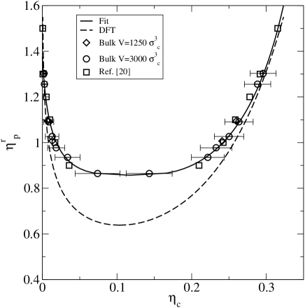
Figure 3: Bulk phase diagram of the AOV model with size ratio $q=\sigma_{\text{p}}/\sigma_{\text{c}}=1$ as a function of the colloidal packing fraction $\eta_{\text{c}}$ and the polymer reservoir packing fraction $\eta_{\text{p}}^{\text{r}}$. Coexistence is along the horizontal tie lines (not shown). Shown are GEMC simulation results for volumes $V=3000\sigma_{\text{c}}^{3}$ (circles) and $V=1250\sigma_{\text{c}}^{3}$ (diamonds), as well as the simulation results from Ref. M. Dijkstra and R. van Roij (2002) (squares). We also display the result of the fit of Eqs. (32) and (33) (solid line) to the simulation data to and the binodal obtained from DFT, or, equivalently, free volume theory (dashed line).

V Results

In this section, we focus on colloid-polymer mixtures with a size ratio $q=1$, a previously well-studied and also experimentally accessible case. We have performed GEMC simulations with $4\times 10^{8}$ steps discarding the initial $10^{8}$ steps for equilibration. The acceptance probability of particle displacement was kept around 10% to 20%, the acceptance probability for volume exchanges was around 50%, while the acceptance probability for transfer of particles was strongly dependent on the statepoint and varied between 50% and 5% for the polymers and from 10% to less than 0.1% for the colloids. The probability of a successful particle transfer typically decreases with increasing particle density. The statistical error of the fugacities serves as a good indicator for the efficiency of the particle transfer between the two boxes; an unreasonably high error indicates that the simulation results are unreliable due to too low particle transfer probabilities. Using this indicator the maximum packing fraction that could be reached in our simulations was $\eta_{\text{c}}\approx 0.34$.

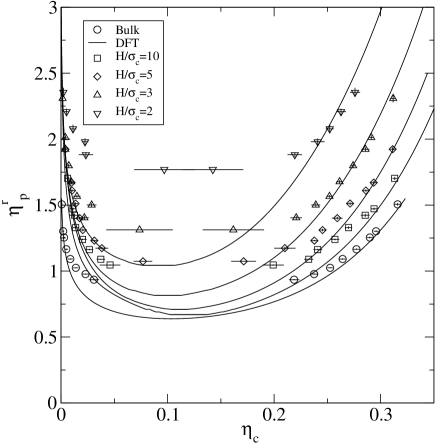
Figure 4: Capillary phase diagram of the AOV model with size ratio $q=\sigma_{\text{p}}/\sigma_{\text{c}}=1$ confined between parallel hard walls with separation distance H/$\sigma_{\text{c}}$=2, 3, 5, 10 and $\infty$ as a function of colloid packing fraction $\eta_{\text{c}}$ and polymer reservoir packing fraction $\eta_{\text{p}}^{\text{r}}$. Shown are results from simulation (symbols) and DFT (continuous lines).

Fig. 3 shows the bulk phase diagram obtained from simulations with a simulation box of volume $V=3000\sigma_{\text{c}}^{3}$. Simulation runs with smaller system sizes display negligible finite size effects. In the $\eta_{\text{c}}$-$\eta_{\text{p}}^{\text{r}}$ representation, the shape of the binodal is similar to that of a simple fluid upon identifying $\eta_{\text{p}}^{\text{r}}$ with inverse temperature. The tielines, connecting the coexisting phases, are horizontal (not shown) as $\eta_{\text{p}}^{\text{r}}$ possesses the same value in the two coexisting phases. We have checked that our results agree well with those obtained by Dijkstra and van Roij M. Dijkstra and R. van Roij (2002) who performed simulations of an effective one component system, which was obtained by formally integrating out the degrees of freedom of the polymers in the partition function.

To estimate the location of the critical point, we fitted the binodals using the scaling law

$$\eta_{\text{c}}^{\text{l}}-\eta_{\text{c}}^{\text{g}}=A\left(\frac{1}{(\eta_{\text{p}}^{\text{r}})_{\text{crit}}}-\frac{1}{\eta_{\text{p}}^{\text{r}}}\right)^{\beta}$$ (32)

and the law of rectilinear diameter

$$\eta_{\text{c}}^{\text{l}}+\eta_{\text{c}}^{\text{g}}=2(\eta_{\text{c}})_{\text{crit}}+B\left(\frac{1}{(\eta_{\text{p}}^{\text{r}})_{\text{crit}}}-\frac{1}{\eta_{\text{p}}^{\text{r}}}\right),$$ (33)

where $\eta_{\text{c}}^{\text{l}}$ is the colloid packing fraction of the coexisting liquid phase, $\eta_{\text{c}}^{\text{g}}$ is the colloid packing fraction of the coexisting gas phase and the subscript $crit$ indicates the value at the critical point. $A$ and $B$ are two free parameters determined from the fit, and $\beta=0.32$ is the three-dimensional Ising critical exponent. We used the standard functional form of the two laws D. Frenkel and B. Smit (2002) but replaced the temperature by the inverse of the polymer reservoir packing fraction. The continuous curve in Fig. 3 is the result of the fit of Eqs. (32) and (33). The fit is remarkably good, but we point out that this only gives an estimate of the critical point. To get a more precise value of the critical packing fractions, it would be necessary to carry out simulations in a region of the phase diagram much closer to the critical point than is possible with GEMC.

In Fig. 3, we also compare our results with those obtained from density functional theory (DFT). We use the approximation for the Helmholtz excess free energy for the AOV model as given in Schmidt et al. (2000). For given external potential, the density functional is numerically minimized using a standard iteration procedure. The discrepancies between theory and simulation can be understood by considering that the DFT for homogeneous (bulk) fluid states of the AOV model is equivalent to the free volume theory of Lekkerkerker et al. H. N. W. Lekkerkerker et al. (1992). Dijkstra et al. M. Dijkstra et al. (1999) showed that this theory is equivalent to a first order Taylor expansion of the free energy around $\eta_{\text{p}}^{\text{r}}=0$

$$\beta F(N_{\text{c}},V,\eta_{\text{p}}^{\text{r}})=\beta F(N_{\text{c}},V,\eta_{\text{p}}^{\text{r}}=0)+$$ (34)

$$+ \int_{\text{0}}^{\eta_{\text{p}}^{\text{r}}}d(\eta_{\text{p}}^{\text{r}})^{\prime}\left(\frac{\partial\beta F(N_{\text{c}},V,(\eta_{\text{p}}^{\text{r}})^{\prime})}{\partial(\eta_{\text{p}}^{\text{r}})^{\prime}}\right)_{(\eta_{\text{p}}^{\text{r}})^{\prime}}$$

$$\simeq \beta F(N_{\text{c}},V,\eta_{\text{p}}^{\text{r}}=0)-\frac{6}{\pi\sigma_{\text{p}}^{3}}\eta_{\text{p}}^{\text{r}}<V_{\text{free}}>_{\eta_{\text{p}}^{\text{r}}=0}\,,$$

neglecting terms ${\cal O}((\eta_{\text{p}}^{\text{r}})^{2})$ and where $\langle V_{\text{free}}\rangle_{\eta_{\text{p}}^{\text{r}}=0}$ is the free volume available for the polymer in the pure hard sphere reference system. It is evident in Fig. 3 that the theory (dashed curve) performs better at high $\eta_{\text{c}}$ where the system is so crowded that it resembles the reference hard sphere system and $\langle V_{\text{free}}\rangle_{(\eta_{\text{p}}^{\text{r}})^{\prime}=0}\simeq\langle V_{\text{free}}\rangle_{(\eta_{\text{p}}^{\text{r}})^{\prime}=\eta_{\text{p}}^{\text{r}}}$. For very small $\eta_{\text{c}}$ the free volume is close to the total volume of the system $V$ for both the pure hard sphere reference system and the actual mixture. For high $\eta_{\text{p}}^{\text{r}}$, the gas-liquid coexistence is very broad and quantitatively well-predicted by the theory. The critical point of the AOV mixture for size ratio $q=1$ is in the region of $\eta_{\text{c}}\sim 0.1$ and the theory underestimates the critical value of $\eta_{\text{p}}^{\text{r}}$. Furthermore, the discrepancy in location of the critical point arises from the mean field critical exponent of the theory against the 3D Ising critical exponent of the simulation R. L. C. Vink and J. Horbach (2004b).

Figure 5: The same as Fig. 4, but as a function of colloid fugacity $z_{\text{c}}\sigma_{\text{c}}^{3}$ and polymer reservoir packing fraction $\eta_{\text{p}}^{\text{r}}$. Statepoint A is in the gas region of the phase diagram for wall separation distances $H/\sigma_{\text{c}}=\infty$, 10, and 5 and in the liquid region of the phase diagram for wall separation distances $H/\sigma_{\text{c}}=3$ and 2. The arrow indicates the direction of the binodal shift upon increasing confinement (decreasing values of $H/\sigma_{\text{c}}$) of the mixture between parallel hard walls.

$H/\sigma_{\text{c}}$	$(\eta_{\text{p}}^{\text{r}})_{\text{crit}}$	$(\eta_{\text{c}})_{\text{crit}}$	DFT $(\eta_{\text{p}}^{\text{r}})_{\text{crit}}$	DFT $(\eta_{\text{c}})_{\text{crit}}$
$\infty$	0.86(1)	0.117(2)	0.638	0.103
10	1.00(1)	0.124(1)	0.670	0.120
5	1.09(1)	0.123(2)	0.710	0.111
3	1.27(2)	0.116(3)	0.815	0.100
2	1.76(2)	0.119(1)	1.044	0.091

Table 1: Capillary critical points of the AOV model between parallel hard walls with separation distance $H/\sigma_{\text{c}}=\infty,10,5,3,$ and 2 obtained from the fit of Eqs. (32) and (33), and from DFT.

V.1 Phase diagrams

First we present the results for the colloid-polymer mixtures confined between two smooth, planar hard walls at distance $H$. In Fig. 4 we show a set of phase diagrams for $H/\sigma_{\text{c}}=\infty$ (bulk), 10, 5, 3, and 2, in the $\eta_{\text{c}}$-$\eta_{\text{p}}^{\text{r}}$ representation. Upon decreasing the plate separation distance $H/\sigma_{\text{c}}$, the critical value of $\eta_{\text{p}}^{\text{r}}$ shifts to higher values, in accordance with the decrease in critical temperature of simple fluids. The theoretical binodals agree well with those from simulation, except close to the critical point. The theory underestimates for all plate separations the critical value of $\eta_{\text{p}}^{\text{r}}$, as it does for the bulk system M. Dijkstra and R. van Roij (2002). We observe that the deviation increases upon decreasing $H/\sigma_{\text{c}}$. In Tab. 1 we show the critical packing fractions obtained from the fit of Eqs. (32) and (33) and from DFT. We used the 3-dimensional Ising critical exponent for all wall separations. Although recent studies Vink et al. (2006) suggests a critical behavior for small wall separations that is neither three-dimensional, nor two-dimensional, the difference is likely to be negligible at the level of precision of our GEMC simulations.

In Fig. 5 we show a set of phase diagrams for $H/\sigma_{\text{c}}=\infty$, 10, 5, 3, and 2 in the $z_{\text{c}}$-$\eta_{\text{p}}^{\text{r}}$ representation. The coexistence gap in colloid packing fractions collapses to a line since two phases at coexistence possess the same colloid fugacity. Note that the system is in the gas phase for fugacity $z_{\text{c}}<z_{\text{c}}^{\text{sat}}$, while it is in the liquid phase for $z_{\text{c}}>z_{\text{c}}^{\text{sat}}$, where $z_{\text{c}}^{\text{sat}}$ denotes the colloid fugacity at bulk coexistence. Statepoint A is gas-like for $H/\sigma_{\text{c}}\geq 5$, but is liquid-like for $H/\sigma_{\text{c}}\leq 3$. Hence, planar slits with $H/\sigma_{\text{c}}\leq 3$ are filled with liquid phase, while the bulk reservoir is in the gas phase, proving the occurrence of capillary condensation upon reducing the width of the slit that is in contact with a bulk gas.

We now turn our attention to colloid-polymer mixtures confined between two smooth, planar semi-permeable walls at distance $H_{\text{c}}$. In Fig. 6 we show a set of phase diagrams for $H_{\text{c}}/\sigma_{\text{c}}=\infty$, 10, 4, and 2 in the $\eta_{\text{c}}$-$\eta_{\text{p}}^{\text{r}}$ representation. Upon increasing the confinement (via reduction of $H_{\text{c}}/\sigma_{\text{c}}$), the critical value of $\eta_{\text{p}}^{\text{r}}$ shifts to higher values. The trend is similar to the behavior of the slit with hard walls, although we find a smaller shift of the critical point (see Tab. 2). In Fig. 7 we show a set of phase diagrams for $H/\sigma_{\text{c}}=\infty,10,4,$ and 2 in the $z_{\text{c}}$-$\eta_{\text{p}}^{\text{r}}$ representation. Statepoint B is liquid-like for $H_{\text{c}}/\sigma_{\text{c}}\geq 10$, but is gas-like for $H_{\text{c}}/\sigma_{\text{c}}\leq 2$. Hence, planar slits with $H_{\text{c}}/\sigma_{\text{c}}\leq 2$ are filled with gas, while the bulk reservoir is in the liquid phase, indicating the occurrence of capillary evaporation.

$H/\sigma_{\text{c}}$	$(\eta_{\text{p}}^{\text{r}})_{\text{crit}}$	$(\eta_{\text{c}})_{\text{crit}}$	DFT $(\eta_{\text{p}}^{\text{r}})_{\text{crit}}$	DFT $(\eta_{\text{c}})_{\text{crit}}$
$\infty$	0.86(1)	0.117(2)	0.638	0.103
10	1.09(2)	0.13(1)	0.660	0.075
4	1.11(4)	0.10(3)	0.699	0.076
2	1.29(1)	0.11(4)	0.818	0.092

Table 2: Capillary critical points of the AOV model between parallel semi-permeable plates with separation distance $H/\sigma_{\text{c}}=\infty,10,4,$ and 2 obtained from the fit of Eqs. (32) and (33), and from DFT.

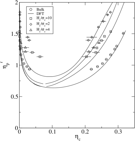
Figure 6: Capillary phase diagram showing the gas-liquid binodal for the AOV model with $q=\sigma_{\text{p}}/\sigma_{\text{c}}=1$ between two parallel semi-permeable walls with separation distances $H_{\text{c}}/\sigma_{\text{c}}$=2, 4, 10, $\infty$ as a function of colloid packing fraction $\eta_{\text{c}}$ and polymer reservoir packing fraction $\eta_{\text{p}}^{\text{r}}$. Shown are results from simulations (symbols) and DFT (lines).

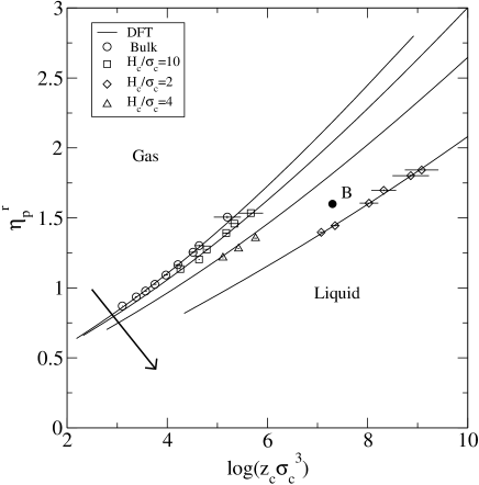
Figure 7: The same as Fig. 6, but as a function of colloid fugacity $z_{\text{c}}\sigma_{\text{c}}^{3}$ and polymer reservoir packing fraction $\eta_{\text{p}}^{\text{r}}$. The arrow indicates the direction of the shift of the binodal upon increasing confinement of the mixture (decreasing values of $H_{\text{c}}/\sigma_{\text{c}}$) between two parallel semi-permeable walls.

V.2 Structure at coexistence

We next analyze the density profiles of both species at capillary coexistence of gas and liquid phases. Such fluid states are translationally invariant against lateral displacements, and the density distributions (of both species) depend solely on the (perpendicular) distance from the walls. We compare theoretical and simulation results for coexistence states at the same values for $\eta_{\text{p}}^{\text{r}}$. In practice, we have used the result for $\eta_{\text{p}}^{\text{r}}$ from the simulations, and have calculated the corresponding DFT profiles. The value for $z_{\text{c}}$ used in the DFT calculations was adjusted according to the respective theoretical capillary binodal. Recall that the quantitative differences in results for the capillary binodals from simulation and theory are small.

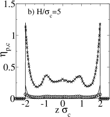
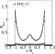
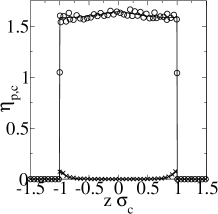
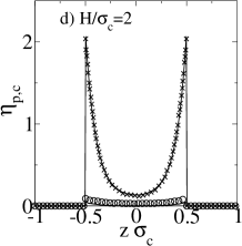
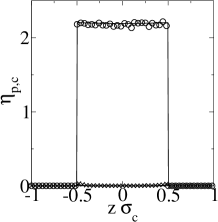
Figure 8: Density profiles of the coexisting liquid (left) and gas (right) phases of the AOV model confined between parallel hard walls with separation distance: a) H/$\sigma_{\text{c}}$=10, at $\eta_{\text{p}}^{\text{r}}$=1.23(1),$z_{\text{c}}\sigma_{\text{c}}^{3}$=66.3(1), b) H/$\sigma_{\text{c}}$=5 at $\eta_{\text{p}}^{\text{r}}$=1.39(1), $z_{\text{c}}\sigma_{\text{c}}^{3}$=99.4(3), c) H/$\sigma_{\text{c}}$=3, at $\eta_{\text{p}}^{\text{r}}$=1.68(1), $z_{\text{c}}\sigma_{\text{c}}^{3}$=128(2), and d) H/$\sigma_{\text{c}}$=2, at $\eta_{\text{p}}^{\text{r}}$=2.23(1), $z_{\text{c}}\sigma_{\text{c}}^{3}$=228(10). Shown are results from simulations for the density profiles of the colloids (crosses) and polymers (circles), along with results from DFT (full lines).

The results for a slit of hard walls are shown in Fig. 8. The colloidal profiles in the liquid phase display strong layering at either wall. For wall separation $H/\sigma_{\text{c}}=10$, at $\eta_{\text{p}}^{\text{r}}=1.23\pm 0.01$, and $z_{\text{c}}\sigma_{\text{c}}^{3}=66.3\pm 0.1$ these oscillations decay to flat, bulk-like behavior in the center of the slit. For smaller wall separations, namely $H/\sigma_{\text{c}}=5$, at $\eta_{\text{p}}^{\text{r}}=1.39\pm 0.01$, and $z_{\text{c}}\sigma_{\text{c}}^{3}=99.4\pm 0.3$, $H/\sigma_{\text{c}}=3$, at $\eta_{\text{p}}^{\text{r}}=1.68\pm 0.01$, and $z_{\text{c}}\sigma_{\text{c}}^{3}=128\pm 2$, and $H/\sigma_{\text{c}}=2$, at $\eta_{\text{p}}^{\text{r}}=2.23\pm 0.01$, and $z_{\text{c}}\sigma_{\text{c}}^{3}=228\pm 10$, we observe the presence of 5, 3, and 2 well-defined layers of particles, respectively. Although their density is much lower, the polymers in the liquid phase display similar behavior. The layering is weaker, but we can observe that a maximum in the colloid profile corresponds also to a maximum in the polymer profile. This result suggests that for such low concentrations polymers behave as hard spheres as packing effects are concerned. In the gas phase, for wall separations $H/\sigma_{\text{c}}=10$ and 5, we find strong adsorption of the colloids at both walls, and a tendency of the polymers to desorb from the walls. In the center of the slit almost no colloids are present and the polymers display flat density profiles with a packing fraction very similar to the polymer reservoir packing fraction. For wall separation distances $H/\sigma_{\text{c}}=3$ and 2, we observe an almost flat polymer density profile, while the density of the colloids is very low throughout the slit. Different from the liquid profiles, a maximum in the colloidal profile corresponds to a minimum of the polymer profiles.

Fig. 9 displays density profiles for the slit of semi-permeable walls. For wall separation distance of $H_{\text{c}}/\sigma_{\text{c}}=10$, at $\eta_{\text{p}}^{\text{r}}=1.39\pm 0.01$, and $z_{\text{c}}\sigma_{\text{c}}^{3}=167\pm 5$, we clearly observe for the liquid state points the presence of a gas layer between the wall and the liquid phase centered in the slit. For wall separation $H_{\text{c}}/\sigma_{\text{c}}=4$, at $\eta_{\text{p}}^{\text{r}}=1.35\pm 0.01$, and $z_{\text{c}}\sigma_{\text{c}}^{3}=318\pm 10$ the gas layers at the walls disappear and indications of layering effects appear. For wall separation $H_{\text{c}}/\sigma_{\text{c}}=2$, at $\eta_{\text{p}}^{\text{r}}=1.61\pm 0.01$, and $z_{\text{c}}\sigma_{\text{c}}^{3}=2950\pm 200$ the colloid density profile displays very significant peaks at both walls. Moreover, we do find layering at larger wall separations, for statepoints well inside the liquid phase. We will discuss this in more detail in the next section. In the gas phase, the density of colloids is very low throughout the slit, while the polymer density profile is almost flat with a packing fraction close to the polymer reservoir packing fraction.

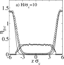
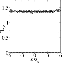
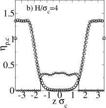
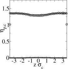
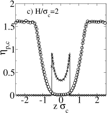
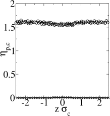
Figure 9: Density profiles of the coexisting liquid (left) and gas (right) phases of the AOV model confined between two parallel semi-permeable walls with varying separation distance: a) H${}_{\text{c}}$/$\sigma_{\text{c}}$=10, at $\eta_{\text{p}}^{\text{r}}$=1.39(1), $z_{\text{c}}\sigma_{\text{c}}^{3}$=167(5), b) H${}_{\text{c}}$/$\sigma_{\text{c}}$=4, at $\eta_{\text{p}}^{\text{r}}$=1.35(1), $z_{\text{c}}\sigma_{\text{c}}^{3}$=318(10), and c) H${}_{\text{c}}$/$\sigma_{\text{c}}$=2, at $\eta_{\text{p}}^{\text{r}}$=1.61(1), $z_{\text{c}}\sigma_{\text{c}}^{3}$=2950(200). Shown are results from simulations for the density profiles of the colloids (crosses) and polymers (circles), and results from DFT (full lines).

The comparison between DFT and simulation indicates good agreement of results from both approaches. Differences in structure can be traced back to differences in the phase diagrams. For fixed $\eta_{\text{p}}^{\text{r}}$ the DFT predicts higher colloid densities and smaller polymer densities, and these differences are reflected by the discrepancies in the profiles. For wall separations where the statepoint is close to the critical point the agreement is worse, especially close to the walls. Such discrepancies between simulation and DFT were previously reported in studying the wall-fluid tension and the adsorption of colloid-polymer mixtures Fortini et al. (2005).

V.3 Structure off-coexistence

We next consider density profiles for a fixed statepoint off-coexistence. For slits with hard walls we chose statepoint A ($\eta_{\text{p}}^{\text{r}}$=1.49 and $\ln(z_{\text{c}}\sigma_{\text{c}}^{3})$=4.6) of Fig. 5, that lies in the stable gas region of the bulk phase diagram. We carried out simulations for wall separation distances $H/\sigma_{\text{c}}=10,5,3,$ and 2. Fig. 10 shows that for wall separations $H/\sigma_{\text{c}}=10$ and 5 the slit is filled with gas. However, for wall separation of $H/\sigma_{\text{c}}=3$ we observe that the capillary fills with liquid. Hence, for this particular statepoint, the critical wall separation distance for capillary condensation lies between 3 and 5 colloid diameters, consistently with the findings of Sec. V.1. Reducing the wall separation to $H/\sigma_{\text{c}}=2$, the liquid phase remains stable. The density profiles in the gas phase possess adsorption peaks in the colloid profile, and corresponding desorption peaks in the polymer profiles. In the liquid phase we observe strong layering of the colloids, and, to a lesser extent, of the polymers. The agreement between simulation and DFT results is good. The differences seem to be related to the vicinity of statepoint A to the critical point. The critical point for wall separation $H/\sigma_{\text{c}}=3$, and 5, is much closer to statepoint A than the critical points for wall separations $H/\sigma_{\text{c}}=10$, and 2, where we find a better agreement between simulation and theory profiles.

We next discuss the structure of the mixture inside the slit with semi-permeable walls (Fig. 11). We fix the fugacities of both species to those at statepoint B ($\eta_{\text{p}}^{\text{r}}$=1.60 and $\ln(z_{\text{c}}\sigma_{\text{c}}^{3})$=7.3), see Fig. 7. The statepoint B is in the liquid part of the bulk phase diagram phase. The liquid fills slits with wall separations $H_{\text{c}}/\sigma_{\text{c}}=10$, and 4, while for $H_{\text{c}}/\sigma_{\text{c}}=2$ the slit is filled with gas. This is an indication of capillary evaporation consistent with the findings of Sec. V.1. The liquid phase is characterized by structureless polymer profiles, and a layering of colloids for both $H_{\text{c}}/\sigma_{\text{c}}=10$, and 4. Note that we did not observe such layering for the statepoints at coexistence (see previous section). Simulation and theory are in good agreement at all wall separations.

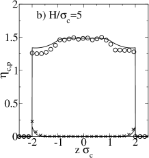
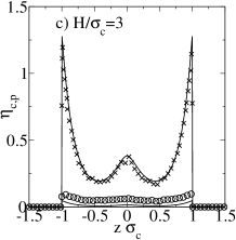
Figure 10: Density profiles of the AOV model with $q=1$ between parallel hard walls with varying separation distance: a) $H/\sigma_{\text{c}}$=10, b) $H_{\text{c}}/\sigma_{\text{c}}$= 5, c) $H_{\text{c}}/\sigma_{\text{c}}$=3, and d) $H_{\text{c}}/\sigma_{\text{c}}$=2 at statepoint A of the phase diagram of Fig. 5, i.e., for polymer reservoir packing fraction $\eta_{\text{p}}^{\text{r}}=1.49$ and colloid fugacity $\ln(z_{\text{c}}\sigma_{\text{c}}^{3})=4.6$. Shown are results from simulations for the density profiles of the colloids (crosses) and polymers (circles), and results from DFT (full lines).

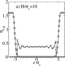
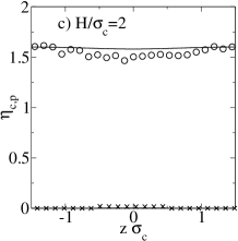
Figure 11: Density profiles of the AOV model between two parallel semi-permeable walls with varying separation distance: a) $H_{\text{c}}/\sigma_{\text{c}}$=10, b) $H_{\text{c}}/\sigma_{\text{c}}$=4, and c) $H_{\text{c}}/\sigma_{\text{c}}$=2 at statepoint B of the phase diagram of Fig. 7, i.e., for polymer reservoir packing fraction $\eta_{\text{p}}^{\text{r}}=1.60$ and colloid fugacity $\ln(z_{\text{c}}\sigma_{\text{c}}^{3})=7.3$. Shown are results from simulations for the density profiles of the colloids (crosses) and polymers (circles), and results from DFT (full lines).

V.4 Two dimensional limit

We next analyze the dimensional crossover from three to two spatial dimensions by reducing the distance of the hard walls towards $H/\sigma_{\text{c}}\rightarrow 1$. The two-dimensional system encountered for $H/\sigma_{\text{c}}=1$ is identical to a two-dimensional mixture of colloidal hard disc and ideal polymer discs. Two-dimensional mixtures were previously studied with both theory J.-T. Lee and M. Robert (1999); M. Schmidt et al. (2002b), and experiments T.-C Lee et al. (2003). For $H$ very close to $\sigma_{\text{p}}$ the polymer reservoir packing fraction scale as

$$\eta_{\text{p}}^{\text{r}}\sim\frac{\pi}{6}\frac{N_{\text{p}}\sigma_{\text{p}}^{3}}{A(H-\sigma_{\text{p}})}.$$ (35)

We eliminate the divergence using scaled variables for the polymer reservoir packing fraction $\eta_{\text{p}}^{\text{r}}(H-\sigma_{\text{p}})/H$ and for the colloidal fugacity $z_{\text{c}}(H-\sigma_{\text{c}})/H$. Effectively, we map the three-dimensional system with packing fractions $\eta_{i}=\pi\sigma_{i}^{3}N_{\text{i}}/(6AH)$ to the two-dimensional system with packing fractions $\eta_{i}=\pi\sigma_{i}^{2}N_{i}/(4A)$, where $i=\text{c, p}$.

In Fig. 12(a) we plot the phase diagrams in the scaled $\eta_{\text{p}}^{\text{r}}-\eta_{\text{c}}$ representation and we observe that the binodals for $H/\sigma_{\text{c}}=1.01$ and $H/\sigma_{\text{c}}=1.005$ are superimposed, demonstrating that this is a reliable estimate for the binodals of the 2-dimensional system. The comparison with a two-dimensional DFT M. Schmidt et al. (2002b) equivalent to a two-dimensional free volume theory J.-T. Lee and M. Robert (1999) indicates poorer agreement as in the three-dimensional case. The discrepancy in the critical polymer reservoir packing fraction is very substantial. We also find that in this representation the binodals of the three-dimensional system of the slits collapse over the bulk binodal, indicating a scaling of the critical value of $\eta_{\text{p}}^{\text{r}}$ as $(\eta_{\text{p}}^{\text{r}})_{\text{crit}}\sim 1/(H-\sigma_{\text{p}})$. In Fig. 12(b) we see that the collapse of the binodals onto a master curve in the scaled $\eta_{\text{p}}^{\text{r}}-$ scaled $z_{\text{c}}$ representation is not as good as in the other representation, moreover the sequence of binodals is inverted, indicating that the critical value of the colloid fugacity scales differently.

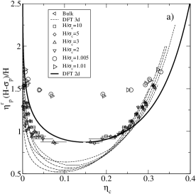
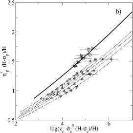
Figure 12: Phase diagrams showing the binodals for the AOV model between parallel hard walls with separation distance $H/\sigma_{\text{c}}=\infty,10,5,3,2,1.01,$ and $1.005$. Shown are results from simulation (symbols), from three-dimensional DFT (dashed curves), and from DFT for the AOV model in two dimensions (full lines). a) The gas-liquid binodal as a function of the scaled variable $\eta_{\text{p}}^{\text{r}}(H-\sigma_{\text{p}})/H$ and $\eta_{\text{c}}$; b) The gas-liquid binodals as a function of the scaled variables $z_{\text{c}}\sigma_{\text{c}}^{3}(H-\sigma_{\text{c}})/H$ and $\eta_{\text{p}}^{\text{r}}(H-\sigma_{\text{p}})/H$.

V.5 Kelvin equation

In this section, we compare the simulation results with the predictions of the Kelvin equations that we derived in section IV. First, we address the relationship of the parameter $h$, we used in the Kelvin equations, to our model parameter $H$. There are two, a priori equivalent, choices that we investigate, namely $h=H$, and $h=H-\sigma_{c}$. Second, the Kelvin equations need, as a input, the difference of the gas and liquid tensions at the wall interface. Since this data are not readily available we will assume, in the case of capillary condensation, the relation $\gamma_{wg}-\gamma_{wl}=\gamma_{lg}$, strictly valid only in the complete wetting regime, to hold at all state points considered. Likewise, for the capillary evaporation case, we assume $\gamma_{wl}-\gamma_{wg}=\gamma_{lg}$, valid in the complete drying regime to hold at all state points. For the liquid-gas interfacial $\gamma_{\rm lg}$ tension we use DFT data from Ref. Brader and Evans (2000).

Figs. 13(a) and 13(c) display the simulation results for the hard wall slit together with the predictions of the Kelvin equations (22), (26), and (31) for $h=H-\sigma_{\text{c}}$, and $h=H$ respectively. The Kelvin equation (22), derived from the path with constant polymer chemical potential, is superimposed at all separation distances with the Kelvin equation (26) derived using the constant pressure path. This is consistent with the observation of Aarts and Lekkerkerker D. G. A. L. Aarts and H. N. W. Lekkerker (2004). Now we can offer an alternative explanation. As shown in Fig 2, for the capillary condensation case the bulk in the gas phase (polymer rich phase), and the path with constant polymer chemical potential is almost equivalent to the constant pressure path. In other words, the bulk reference point for Eq. (22) and Eq. (26) is very similar in the case of capillary condensation. The Kelvin equation (31) derived using a normal path, predict a smaller shift with respect to Eq. (26). To estimate the error introduced by the complete wetting approximation ($\gamma_{wg}-\gamma_{wl}=\gamma_{lg}$), we show few points (filled diamonds) predicted by Eq. (26) using the actual difference in wall tensions, as published in our previous work M. Schmidt et al. (2003).

The Figs. 13(b) and 13(d) display the simulation results for the semi-permeable wall slit together with the predictions of the Kelvin equations (22), (27), and (31) for $h=H-\sigma_{\text{c}}$, and $h=H$ respectively. The prediction of Eq. (27) and (31) are superimposed at all separation distances considered. This is surprising since they are derived from very different ”paths”, as shown in Fig. 2.

We can conclude that the Kelvin equation we derived using a novel approach, gives predictions that are consistent, and in quantitatively agreement with the prediction of the classic equation. In addition our equation is the same for capillary condensation and evaporation, and the choice of reference state, which is different for both phenomena, is avoided. As the Kelvin equation is based on macroscopic arguments, is surprising that we find reasonable quantitative agreement for nearly two-dimensional systems. The shift of the critical polymer fugacity towards higher values upon increasing confinement, as found in simulations, is not reproduced, because the Kelvin equation is entirely based on properties of the (semi)infinite system. Finally, the two choices of $h$ we presented give essentially the same results for wall separations H$/\sigma_{c}$ as small as 4.

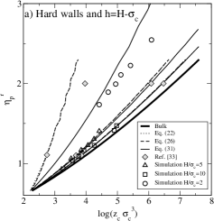
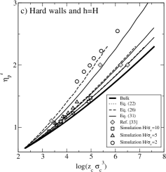
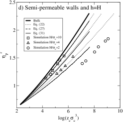
Figure 13: Phase diagram of colloid-polymer mixtures in the colloidal chemical potential $\log(z_{\text{c}}\sigma^{3}_{\text{c}})$ and the polymer reservoir packing fraction $\eta_{\text{p}}^{\text{r}}$ representation. a) Results for slits with hard walls, and $h=H-\sigma_{c}$. b) Results for the slit with semi-permeable walls , and $h=H-\sigma_{c}$. c) Results for the slits with hard walls, and $h=H$. d) Results for the slit with semi-permeable walls, and $h=H$. In a) and c) the simulation results (symbols) are compared with the prediction of the Kelvin equations (22), (26), and (31) assuming complete wetting ($\gamma_{wg}-\gamma_{wl}=\gamma_{lg}$). The filled diamonds are results from Eq. (26) using the difference in wall tensions $\gamma_{wg}-\gamma_{wl}$ taken from Ref. M. Schmidt et al. (2003). In b) and d) the simulation results (symbols) are compared with the prediction of the Kelvin equations (22), (27), and (31) assuming complete drying ($\gamma_{wl}-\gamma_{wg}=\gamma_{lg}$). For the liquid-gas interfacial tension $\gamma_{\rm lg}$ we used DFT data from Ref. Brader and Evans (2000). Few lines are superimposed, see text for the explanation.

VI Conclusions

In conclusion, we have studied the effect of strong confinement provided by two parallel walls on the phase behavior and structure of model mixtures of colloids and polymers of size ratio $q=1$. The densities of the gas and liquid phases at coexistence, as well as the chemical potentials were computed by GEMC simulations and DFT. Two different models of confining walls were investigated: i) Hard walls, impenetrable to both colloids and polymers, as a model for glass walls in contact with colloid-polymer mixtures were found to stabilize the liquid phase for statepoints that lie in the gas part of the bulk phase diagram; this effect is referred to as capillary condensation. ii) Semi-permeable walls, impenetrable to colloids but penetrable to polymers, could be experimentally realized using polymer coated substrates W. K. Wijting et al. (2003b). If the coating density is not too high the polymer brushes can act as impenetrable for colloids while being penetrable for polymers. We find that the effect of semi-permeable walls is to stabilize the gas phase for statepoints in the liquid part of the bulk phase diagram; this effect is referred to as capillary evaporation. Both capillary evaporation and condensation are consistently predicted by GEMC simulations and DFT. The differences between simulations and DFT in the vicinity of the critical point are confirmed for bulk mixtures and were found to be larger for the confined mixtures. The differences reach a maximum in the limit of two-dimensional colloid-polymer mixtures.

We have studied the structure of the mixture between parallel walls by measuring the density profiles in the direction normal to the confining walls. For the liquid phase, rich in colloids and poor in polymers, we found layering of colloids with an oscillation period roughly equal to the diameter of the particles for all wall separations and statepoints considered. In the case of semi-permeable walls, the structure, i.e. the layering of colloids and the adsorption or desorption of gas layers at the semi-permeable walls, depends strongly on the statepoint and on the lengthscale of the confinement. For the gas phase, rich in polymers and poor in colloids, we found flat polymer profiles with moderate desorption of polymers from the hard walls. We found that density oscillations for colloids and polymers are correlated in the liquid phase and anti-correlated in the gas phase. This can be understood by the following argument. In the liquid phase the fraction of polymers is small and a polymer is always surrounded by other colloids to which it interacts with an hard-core potential. Clearly the polymer structure must be similar to that of the colloids. In the gas phase the fraction of polymers is large with respect to the colloids and the entropy is increased by segregation of colloids, so if a region is locally denser in polymer than the average polymer density, it will be more dilute in colloids. The comparison between simulation and DFT is overall good, with small differences in the vicinity of the critical point. Our findings of capillary condensation for hard walls and capillary evaporation for semi-permeable walls are consistent with the experimental findings of Aarts et al. D. G. A. L. Aarts and H. N. W. Lekkerker (2004) and Wijting et al. W. K. Wijting et al. (2003a, b). Nevertheless the comparison is only qualitative. Experiments with better controlled geometries are needed to relate directly to our predictions. The use of the surface force apparatus, for example, should be possible for colloid-polymer mixtures. Simulations and theory should proceed to more realistic models for colloid-polymer mixtures Bolhuis et al. (2002); Vink and Schmidt (2005); Vink et al. (2005). For example, the inclusion of excluded volume interactions between polymer coils has given accurate results for the bulk phase diagram Bolhuis et al. (2002). The use of realistic models for confined mixtures should help understanding the surface phase behavior of real colloid-polymer mixtures. Work along this line is in progress.