Signature of the electron-electron interaction in the magnetic field dependence of nonlinear I-V characteristics in mesoscopic conductors

Abstract

The nonlinear I-V characteristics of mesoscopic samples contain parts which are linear in the magnetic field and quadratic in the electric field. These contributions to the current are entirely due to the electron-electron interaction and consequently they are proportional to the electron-electron interaction constant. We present detailed calculations of the magnitude of the effect as a function of the temperature, and the direction of the magnetic field. We show that in the case of a magnetic field oriented parallel to the sample, the effect exists entirely due to spin-orbit scattering. The temperature dependence of the magnitude of the effect has an oscillating character with a characteristic period on the order of the temperature itself. We also clarify in this article the nature of the electron-electron interaction constant which determines the magnitude of the effect.

I Introduction

According to Onsager, the linear conductance $G(\mathbf{H})$ of a conductor measured by the two-probe method must be an even function of the magnetic field $\mathbf{H}$ Landau :

$$G(\mathbf{H})=G(-\mathbf{H})$$ (1)

This is a consequence of general principles: the time reversal symmetry and the positive sign of the entropy production. Therefore it holds in all nonmagnetic conductors. In a single particle approximation and at zero temperature the validity of Eq. 1 also can be verified using the Landauer formula for the conductance of a sample

$$G=\frac{e^{2}}{h}\sum_{ij}|T_{ij}(\mathbf{H})|^{2}$$ (2)

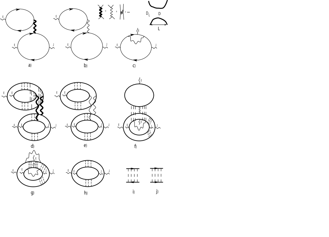
Figure 1: Diagrams describing $I_{nl}$, and $\langle I_{nl}^{2}\rangle$. Thin thin solid lines correspond to the electron green functions, thick solid lines correspond to electron Green functions averaged over random realizations of the scattering potential, dashed lines correspond to the correlation function of the scattering potential given by Eq. 18 . The fat wiggly line is the effective electron interaction interaction, thick wiggly lines correspond to the elecron-electron interaction $V(\mathbf{r})$. Diagrams b,c corresponds to Hartree (b ) and Fock (c) terms of the perturbation theory with respect to $V(\mathbf{r})$.

and requirement of time reversal symmetry $T_{ij}(\mathbf{H})=T_{ji}^{\ast}(-\mathbf{H)}$. Here $T_{ij}$ is a scattering matrix between electronic channels labelled by the indices $i$ and $j$ (see for review of the subject Ref. binnakker ). To verify the validity of Eq. 1 in mesoscopic samples AltshulerKhmelnitski one has to prove that $\langle(G(\mathbf{H})-G(-\mathbf{H}))^{2}\rangle=0$, which requires the cancellation of the odd-in-$\mathbf{H}$ parts of the Cooperon and Diffuson type of diagrams shown in Fig. 1h,i,j. Here the brackets $\langle\rangle$ denote averaging over random realizations of the impurity potential (we use standard diagram technique for averaging over random scattering potential Abricosov ).

On the other hand there are no general principles preventing the existence of odd-in-$\mathbf{H}$ terms in the nonlinear I-V characteristics of conductors. In this article we study the quadratic-in-voltage $V$ part of the I-V characteristics which can be represented as

$$I_{(nl)}=V^{2}[F_{o}(\mathbf{H})+F_{e}(\mathbf{H})]$$ (3)

where $F_{o}(\mathbf{H})$ and $F_{e}(\mathbf{H})$ are odd and even functions of $\mathbf{H}$ respectively. Since $\mathbf{H}$ is an axial vector and the current density, $\mathbf{j}$, is a polar one, the function $F_{o}(\mathbf{H})$ can be non-zero only in non-centro-symmetric media. It is important to study $F_{o}(\mathbf{H})$ because of the fact that in the approximation of noninteracting electrons, $F_{o}(\mathbf{H})=0$. It is particularly simple to verify this fact using the Landauer formula. Indeed, in the absence of the electron-electron or electron-phonon interactions, the total current through the sample will be the sum of contributions from different electron energies. Each of these contributions is an even function of $\mathbf{H}$, and hence the total current will also be an even function of $\mathbf{H}$. Thus the effect is entirely due to electron-electron or electron-phonon interaction. In contrast, the even-in-$\mathbf{H}$ function $F_{e}(\mathbf{H})$ can be described even in a single particle approximation (see, for example, Ref. LarkinKhmelnitskii where the calculations were done in the case of mesoscopic samples).

In the case of pure bulk non-centro-symmetric crystals, and at high temperatures the effect described by $F_{o}(\mathbf{H})$ has been investigated both theoretically and experimentally (see, for example, Ref. Photovoltaic ). In the case of chiral carbon nanotubes a classical theory of this effect was discussed in Ref. ivchenko . At high temperatures there are two contributions to the effect:

a) The first contribution is purely classical and it can be described in the framework of the Boltzmann kinetic equation: An electric field accelerates electrons creating a non-equilibrium distribution function. This non-equilibrium distribution function consists of two parts: an anisotropic-in-momentum part that is proportional to $V$ and a quadratic-in-$V$ contribution which is isotropic in the momentum. In isotropic media, the relaxation of this non-equilibrium distribution due to inelastic scattering processes yields no net current; however, in non-centrosymetric media and in the presence of the magnetic field, the inelastic relaxation rate has odd in electron momentum components, which give rise to the odd-in-$\mathbf{H}$ part of Eq. 3 described by $F_{o}(\mathbf{H})$.

b) The second contribution BelinicherIvchenko is due to a shift in the center of mass of a wave-packet during collisions. The description of these processes is beyond the classical Boltzmann kinetic equation. In non-equilibrium and non-centro-symmetric media and in the presence of the magnetic field these shifts take place in a particular direction determined by a crystal symmetry, and lead to an odd in $\mathbf{H}$ contribution in the net current through the sample. This contribution is similar to that discussed in the framework of the anomalous Hall effect Hall . The above two contributions to $F_{o}(\mathbf{H})$ are proportional to the inelastic electron relaxation rate $1/\tau_{\epsilon}$, and consequently, they vanish at $T=0$ (there are of course contributions from the above effect to the I-V characteristics which at $T=0$ are proportional to higher powers of $V$).

It has been pointed out in Refs. Buttiker ; SpivakZyuzin1 that in mesoscopic metallic samples, where all spatial symmetries are broken, there is an odd-in-$\mathbf{H}$ contribution to Eq. 3 which survives in the limit $T=0$ and which therefore determines the magnitude of the effect at small $T$. This effect has been observed experimentally Cobden ; Markus ; Leturcq ; Marlow ; Helene . As usual for mesoscopic effects, this contribution is due to random electronic interference. Therefore it exhibits random sample specific oscillations as a function of the external magnetic field, temperature and the electron chemical potential. The characteristic feature of the effect is that it is proportional to the amplitude of the electron-electron interaction rather than the scattering rate. The qualitative explanation of the effect is the following SpivakZyuzin1 : The linear in $V$ mesoscopic fluctuations of the current density are due to random interference of electron waves travelling along different diffusive paths. Though the total current through the sample should be an even function of $\mathbf{H}$, the local current densities contain a part which is odd-in-$\mathbf{H}$. By the same token, there is a part of the electron density $\Delta n(\mathbf{r},V,\mathbf{H})$ which is proportional to $V$ and odd-in-$\mathbf{H}$ SpivakZyuzin . In the presence of the spin-orbit scattering the applied voltage also induces local fluctuations of the spin density $\Delta\mathbf{S}(\mathbf{r},V,\mathbf{H})$. These nonequilibrium densities create an additional random potential due to electron-electron interaction

$$\Delta u(\mathbf{r},V,\mathbf{H})=\beta_{eff}^{(1)}\Delta n(\mathbf{r},V,\mathbf{H})$$ (4)

and an additional exchange magnetic field

$$\mathbf{h}(\mathbf{r},V,\mathbf{H})=\beta_{eff}^{(2)}\Delta\mathbf{S}$$ (5)

were $\beta_{eff}^{(1,2)}$ are interaction constants. We can then calculate a change of a linear conductance of a sample, $\Delta G=G(\{u(\mathbf{r)}+\Delta u(\mathbf{r}),\mathbf{h}(\mathbf{r})\})-G(\{u\})$, induced by a change of the scattering potential given by Eq. 4, which gives us

$$I_{(nl)}=\Delta G[V,\mathbf{H},\{\Delta u(\mathbf{r},V,\mathbf{H}),\mathbf{\ h}(\mathbf{r},V,\mathbf{H})\}]V$$ (6)

Expanding Eq. 6 with respect to $\Delta u(\mathbf{r})$ , and $\mathbf{h}(\mathbf{r})$ we arrive at Eq. 3.

In this paper, we present calculations of the magnitude of the effect as a function of the temperature and the magnetic field. We show that in the case of parallel magnetic field, the effect exists entirely due to spin-orbit scattering. The temperature dependence of the magnitude of the effect (both in parallel and in the perpendicular magnetic field) randomly oscillates with a characteristic period on the order of the temperature itself. We also take into account the exchange contribution to the effect and clarify the nature of the electron-electron interaction constant which determines the value of $F_{o}(\mathbf{H})$ in Eq.3.

II Diagrammatic calculations of the magnitude of the effect

Let us consider a sample shown in the insert of Fig.1 with the characteristic size $L$ which is much larger than the electron elastic mean free path $l$. In this limit $\langle I_{nl}\rangle=0$. Therefore we shall characterize the magnitude of the current by the variance $\langle I_{nl}^{2}\rangle$. Before averaging over random potential configurations, to first order in the electron-electron interaction constant, the value of $I_{nl}$ is given by the diagram shown in Fig. 1a. After averaging, the quantity $\langle I_{nl}^{2}\rangle$ is given by diagrams shown in Fig. 1d. In these diagrams, the solid lines which correspond to the electron Green functions carry frequencies on the order of the temperature $T$, so we can neglect frequency dependence of interaction propagators. Thus one can introduce an additional scattering scalar potential given by Eqs. 4, 5 substitute it into Eq. 6, and arrive at Eq. 3.

Generally $\beta_{eff}^{(1)}$ and $\beta_{eff}^{(2)}$ are phenomenological parameters represented by thick wiggly lines in Fig.1a,d. At high electron density, electrons are weakly interacting. In this limit the diagram in Fig. 1a is reduced to those shown in Fig.1b,c. These diagrams correspond to the Hartree and Fock contributions respectively. This means that $\beta_{eff}^{(1,2)}$ can be calculated to first order in perturbation theory with respect to the electron-electron interaction $V(\mathbf{r})$

$$\beta_{eff}^{(1)}=V(0)-\frac{1}{2}\overline{V(k_{F}(\mathbf{\hat{n}-\hat{n^{\prime}}}))}$$

$$\beta_{eff}^{(2)}=\frac{1}{2}\overline{V(k_{F}(\mathbf{\ \hat{n}-\hat{n^{\prime}}}))}$$ (7)

where $V(\mathbf{q})$ is a Fourier transform of a screened Coulomb interaction. The bar denotes the average over the angle of the unit vectors $\mathbf{n}$, and $\mathbf{n}^{\prime}$. To verify this fact one has to show that diagrams Fig.1e,f,g contains only combinations $\left(V(0)-\frac{1}{2}\overline{V(k_{F}(\mathbf{\hat{n}-\hat{n^{\prime}}}))}\right)^{2}$ and $\left(\frac{1}{2}\overline{V(k_{F}(\mathbf{\ \hat{n}-\hat{n^{\prime}}}))}\right)^{2}$.

The system of equations 4,5,6,7 is a generalization of that in Ref. SpivakZyuzin1 where only Hartree term was taken into account. Eq. 7 is typical for many effects in mesoscopic conductors with interacting electrons (see for example AronovAltshuler ; Aleiner ). Usually, however, electron-electron interaction effects give small corrections to the conductance of good conductors with $G\gg e^{2}/\hbar$. In our case, the magnitude of the effect is proportional to $\beta_{eff}$.

To get Eq. 3 one has to expand the expression for the conductance in Eq. 6 with respect to $\Delta u(\mathbf{r})$ and $\mathbf{h}(\mathbf{r})$. To do so it is convenient to expand the potential ZyuzinSpivakNL

$$\Delta u(\mathbf{r})=\sum_{i}^{\infty}u_{i}n_{i}(\mathbf{r})$$ (8)

and the effective magnetic field

$$h_{\alpha}(\mathbf{r})=\sum_{i}^{\infty}h_{\alpha,i}n_{i}(\mathbf{r})$$ (9)

in a complete set of orthogonal eigenstates $n_{i}(\mathbf{r})$ of the diffusion equation $(\int d\mathbf{r}n_{i}^{2}(\mathbf{r})=1)$:

$$D\frac{\partial^{2}}{\partial^{2}\mathbf{r}}n_{i}(\mathbf{r})=E_{i}n_{i}(\mathbf{r})$$ (10)

where $E_{i}$ are the eigenvalues of Eq.10, and $i$ labels the eigenstates. We assume boundary conditions, which correspond to zero current through a closed boundary, and $n_{i}(\mathbf{r})=0$ at the open boundary. Generally speaking the electron density $\Delta n(\mathbf{r})$ and, consequently $\Delta u(\mathbf{r})$ contain all spatial harmonics, and the problem is similar to the sensitivity of the sample conductance to a change in the scattering potential $\Delta u(\mathbf{r})$ considered in LeeStone ; AltshulerSpivak . Thus we have

$$F_{o}(\mathbf{H})=\frac{1}{2V}\sum_{i}\frac{dG(u_{i})}{du_{i}}(u_{i}(\mathbf{H})-u_{i}(\mathbf{-H}))+\frac{1}{2V}\sum_{i,\alpha}\frac{dG}{dh_{i,\alpha}}(h_{i,\alpha}(\mathbf{H})-h_{i,\alpha}(\mathbf{-H}))$$ (11)

In the absence of the spin-orbit scattering the second term in Eq.11 is zero while $dG/du_{i}$ is an even function of $\mathbf{H}$. Thus in this case the effect originates from the odd in $\mathbf{H}$ part of $\Delta n(\mathbf{r},V,\mathbf{H})$. In the presence of the spin-orbit scattering the second term is nonzero and there is another contribution to the effect which comes from the odd-in-$\mathbf{H}$ part of $\mathbf{h}(\mathbf{r},V,\mathbf{H})$. Using Eq. 11 and neglecting small correlations between $\Delta G$, $\Delta u(\mathbf{r})$ and $\mathbf{h}(\mathbf{r})$ we get

$$\langle F_{o}^{2}\rangle = \frac{1}{4V^{2}}\sum_{i,j}\langle\frac{dG}{du_{i}}\frac{dG}{du_{j}}\rangle\langle(u_{i}(\mathbf{H})-u_{i}(-\mathbf{H}))(u_{j}(\mathbf{H})-u_{j}(-\mathbf{H}))\rangle+$$ (12)

$$\frac{1}{4V^{2}}\sum_{i,j,\alpha,\beta}\langle\frac{dG}{dh_{i,\alpha}}\frac{dG}{dh_{j,\beta}}\rangle\langle(h_{i,\alpha}(\mathbf{H})-h_{i,\alpha}(\mathbf{-H}))(h_{j,\beta}(\mathbf{H})-h_{j,\beta}(\mathbf{-H}))\rangle$$

Eq. 12 only contains correlation functions which can be estimated in a single particle approximation (in zero order in $V(\mathbf{r})$). This can be done in a standard way (see for example AronovAltshuler ; LeeStone ; SpivakZyuzin ) by calculating diagrams shown in Fig.1e,f,g. These diagrams contain ladder parts, shown in Fig.1i,j, which depend on the electron spin indices. After summation over the spin indices, the diagrams shown in Fig.1e,f,g only contain the blocks $P_{i}(\mathbf{r,r}_{1}\mathbf{,}\epsilon_{12}\mathbf{,H,}\omega_{s})$ $(i=1,2,3)$ described by the equations

$$\begin{array}[]{c}\left(-D\left(\mathbf{\nabla}+i\frac{e}{c}\mathbf{A}\right)^{2}+i\omega+i\omega_{s}sign\omega+\tau_{\varphi}^{-1}\right)P_{1}(\mathbf{r,r^{\prime},}\omega\mathbf{,H,}\omega_{s})+\frac{1}{2\tau_{so}}\left(P_{1}-P_{2}\right)=\delta\left(\mathbf{r}-\mathbf{r}^{\prime}\right)\\ \left(-D\left(\mathbf{\nabla}+i\frac{e}{c}\mathbf{A}\right)^{2}+i\omega-i\omega_{s}sign\omega+\tau_{\varphi}^{-1}\right)P_{2}(\mathbf{r,r^{\prime},}\omega\mathbf{,H,}\omega_{s})+\frac{1}{2\tau_{so}}\left(P_{2}-P_{1}\right)=0\\ \left(-D\left(\mathbf{\nabla}+i\frac{e}{c}\mathbf{A}\right)^{2}+i\omega+\frac{1}{\tau_{so}}+i\omega_{s}sign\omega+\tau_{\varphi}^{-1}\right)P_{3}(\mathbf{r,r^{\prime},}\omega\mathbf{,H,}\omega_{s})=\delta\left(\mathbf{r}-\mathbf{r}^{\prime}\right)\end{array}$$ (13)

Here $\tau_{so}$ is the spin-orbit mean free time. These equations account for the dependence of $P_{i}$ on spin-orbit scattering and magnetic field. The magnetic field enters through the vector potential $\mathbf{A}$ and the Zeeman splitting $\omega_{s}=g\mu_{B}H$, where $\mu_{B}$ is the Bohr magneton. The boundary condition for these diffusion poles at the insulating boundary is $\mathbf{n}\left(\mathbf{\nabla}+i\frac{e}{c}\mathbf{A}\right)P_{i}(\mathbf{r,r^{\prime},}\omega\mathbf{,H,}\omega_{s})=0$. In the case of ideal leads, when the electron diffusion coefficient in the leads is infinite, the boundary condition at the leads is $P_{i}(\mathbf{r,r^{\prime},}\omega\mathbf{,H,}\omega_{s})=0$. The quantities $P_{i}(\mathbf{r,r}_{1}\mathbf{,}\epsilon_{12}\mathbf{,H,}\omega_{s})$ enter expressions for $I_{nl}$ only in the combination

$$\begin{array}[]{c}\sum_{i=1,2}\left(P_{i}(\mathbf{r,r}_{1}\mathbf{,}\epsilon_{12}\mathbf{,}0,0)P_{i}(\mathbf{r}_{1}\mathbf{,r,}\epsilon_{21}\mathbf{,}0,0)-P_{i}(\mathbf{r,r}_{1}\mathbf{,}\epsilon_{12},2\mathbf{H,}\omega_{s})P_{i}(\mathbf{r}_{1}\mathbf{,r,}\epsilon_{21},2\mathbf{H,}\omega_{s})\right)+\\ +P_{3}(\mathbf{r,r}_{1}\mathbf{,}\epsilon_{12}\mathbf{,}0,\omega_{s})P_{3}(\mathbf{r}_{1}\mathbf{,r,}\epsilon_{21}\mathbf{,}0,\omega_{s})-P_{3}(\mathbf{r,r}_{1}\mathbf{,}\epsilon_{12},3\mathbf{H,}0)P_{3}(\mathbf{r}_{1}\mathbf{,r,}\epsilon_{21},3\mathbf{H,}0)\end{array}$$ (14)

It is convenient to choose the gauge $\mathbf{nA}=0$ at insulating boundary. In this gauge, when calculating magnetic field dependence we can use standard perturbation theory with respect to the magnetic field.

The sum over $i$ in Eq. 12 converges quickly and, consequently, the main contribution comes from the zero-harmonic with $i\sim 0$ (this fact is related to the long range character of the correlation function of the part of the electron densities which are proportional to $V$ SpivakZyuzin ). Consequently the approximation where only this zero harmonic of the potential

$$u_{0}(V,\mathbf{H})=\frac{\beta_{eff}}{v}\int_{v}\Delta n(\mathbf{r},V,\mathbf{H})d\mathbf{r}$$ (15)

is taken into account gives a result valid in order of magnitude. In this formula, $v$ is the volume of the sample, which reduces to $A$, the area of the sample, in the two-dimensional case. In the case when $r_{s}\ll 1$ $\beta_{eff}^{\left(1\right)}\gg\beta_{eff}^{\left(2\right)}$ we also can neglect the exchange field $\mathbf{h}(\mathbf{r},V,\mathbf{H})$ .

In the rest of the article we consider the case of a two-dimensional sample which has a thickness much smaller that its lateral dimension, $L\gg L_{z}$. In this case the results are different for cases of a perpendicular and a parallel magnetic field.

II.0.1 Effect in a Perpendicular Magnetic Field

In the case where the magnetic field is oriented perpendicular to the film, spin-orbit scattering can be neglected as long as $\tau_{so}\gg\tau$. In this case the result depends on the relations between the sample size $L$, the magnetic length $L_{H}$, the dephasing length $L_{\varphi}$, and the thermal coherence length of normal metal $L_{T}$. It also depend on the nature of the leads to the sample.

Let us start with the case of ideal leads when the electron diffusion coefficient in the leads is infinite, $D_{L}=\infty$.

Then at small temperatures $L_{T},L_{\varphi}\gg L$ we get

$$\langle F_{o}^{2}(\mathbf{H})\rangle=BH^{2}(\beta_{eff}^{(1)})^{2}\frac{e^{2}}{\hbar^{2}\Gamma^{4}A^{2}}\bigg{(}\frac{e^{2}}{h}\bigg{)}^{2}\bigg{(}\frac{L^{2}}{\Phi_{0}}\bigg{)}^{2}$$ (16)

where $\Gamma=D/L^{2}$, $D=v_{F}l/2$ is the diffusion coefficient inside a two-dimensional sample, $B$ is a numerical factor of order one, and $A$ is the area of the sample.

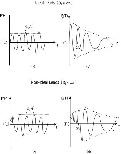
Figure 2: Qualitative pictures of $H$- and $T$ dependencies of $F_{0}(H,T)$. Figs. a) and b) correspond to the case of ideal leads ($D_{L}=\infty$), while Figs. c and d correspond to the case of diffusive leads $D_{L}<\infty$ .

The linear $H$-dependence of $I_{nl}$ given by Eq. 16 holds at small magnetic fields when $HL^{2}\ll\Phi_{0}$, where $\Phi_{0}=\hbar e/c$ is the flux quanta. In the opposite limit $HL^{2}\gg\Phi_{0}$ the function $F_{o}(\mathbf{H})$ exhibit random oscillations as a function of $H$ with a characteristic period of order $\Delta H\sim\Phi_{0}/L^{2}$. To verify this one can show that the correlation function $\langle F_{o}(H+\Delta H)F_{o}(H)\rangle$ decays at $\Delta H\sim\Phi_{0}/L^{2}$. Qualitatively the dependence $F_{o}(\mathbf{H})$ in the case $D_{L}=\infty$ is shown in Fig. 2a.

The temperature dependence of $F_{o}(\mathbf{H},T)$ is nontrivial because it exhibit random oscillations as a function of $T$ which are shown qualitatively in Fig. 2b. To verify this one has to calculate two correlation functions

$$\langle F_{o}^{2}(T)\rangle\sim\langle F_{o}(0)F_{o}(T)\rangle$$ (17)

and notice that they have the same temperature dependencies. It also follows from Eq. 17 that at $T>D/L^{2}$, the period of oscillations is on the order of the temperature itself. Let us turn now to the case when the leads have the same diffusion coefficient as the sample, $D_{L}=D$. In this case $H$ and $T$ dependencies of $F(H,T)$ are qualitatively shown in Figs. 2c,d. The main difference with the case $D_{L}=0$ is that in this case $F_{o}(T,H)$ exhibits random oscillations as functions of $H$ and $T$ even in the case $L_{H}\gg L$ and $L_{T}\gg T$. These oscillations are related to the existence of diffusive electron trajectories which leave the sample, travel in the leads and then come back. Their contribution to the total current is small, but their sensitivity to changes of $H$ and $T$ are so big that the derivatives $\partial F_{o}/\partial T\rightarrow\infty$ and $\partial F_{o}/\partial H\rightarrow\infty$ at zero temperature and magnetic field $H\rightarrow 0$. Qualitatively the $T$ and $H$ dependencies of $F_{o}(T,H)$ are similar of those of the linear conductance LeeStone ; ZyuzinSpivakH ; CobdenSpivakZyuzin .

II.0.2 Effect in a Parallel Magnetic Field

When deriving Eq. 16 we neglected the effect of Zeemann splitting of the electron spectrum because it gives a small contribution to the effect. However, when a thin enough sample is oriented parallel to a magnetic field $\mathbf{H}_{\|}$, the orbital contribution of the magnetic filed is absent, and Zeemann splitting causes the dominant contribution to $I_{nl}$. However, in the absence of spin-orbit scattering, $\delta n(\mathbf{H}_{\|})$ , and consequently $I_{nl}$ are even functions of $\mathbf{H}_{\|}$. Thus in this case the effect is determined by the spin-orbit scattering rate $1/\tau_{so}$. In the presence of spin-orbit scattering the dashed lines in Fig.1 correspond to the following expression

$$\frac{1}{2\pi\nu\tau}\delta_{\alpha\beta}\delta_{\delta\gamma}+\frac{1}{8\pi\nu\tau_{so}}\mathbf{\sigma}_{\alpha\beta}\mathbf{\sigma}_{\delta\gamma}$$ (18)

In the case of a weak magnetic field, $\mathbf{\mu_{B}\cdot H_{\|}}\ll 1/\tau_{so},\Gamma$, and at $T=0$, we get an expression for the odd-in-$\mathbf{H}_{\|}$ part of the zero mode of the density fluctuation

$$\langle F_{o}^{2}(\mathbf{H}_{\|})\rangle=C\left(\frac{e^{2}}{h}\right)^{2}\frac{e^{2}}{\hbar^{2}A^{2}\Gamma^{2}}\left(\beta_{eff}^{(1)}\right)^{2}\frac{1}{\tau_{so}}\frac{1}{\Gamma\left(\Gamma+\frac{1}{\tau_{so}}\right)^{4}}\left[2\Gamma^{2}+2\Gamma\frac{1}{\tau_{so}}+\frac{1}{\tau_{so}^{2}}\right]\left(\frac{\mu_{B}\mathbf{H}_{\|}}{\Gamma}\right)^{2}$$ (19)

where $C\sim 1$. In the case of weak spin-orbit scattering $\Gamma\gg\tau_{so}^{-1}$ we have $\langle F_{o}^{2}\rangle=\Gamma^{-7}$. It is interesting that the amplitude of the effect is proportional to the amplitude of the spin-orbit scattering rather than it’s rate. This expression holds as at $\mu_{B}H_{\|}<\Gamma$. In the opposite limit we have $\langle F_{o}^{2}\rangle=\Gamma^{-5}$ which is independent of $\mathbf{H}_{\|}$. In this region $F_{o}(\mathbf{H}_{\|})$ exhibit random sample specific oscillations as a function of $H_{\|}$ with a characteristic period of order $\Gamma/\mu_{B}$. To get this result one has to calculate the correlation function $\langle\left[F_{o}(\mathbf{H}_{\|})-F_{o}(\mathbf{H_{\|}+\Delta H_{\|}})\right]^{2}\rangle$ and to see that it decays at $\mu H_{\|}>\Gamma$.

In the limit of a strong spin-orbit scattering $\Gamma,\mu_{B}\mathbf{H}_{\|}\ll 1/\tau_{so}$ we have $\langle F_{o}^{2}\rangle\sim 1/\tau_{so}$ , and the amplitude of the effect which decreases as $\tau_{so}$ increases. In the limit of strong magnetic field $\mu_{B}\mathbf{H}_{\|}\gg 1$ we have $\langle F_{o}^{2}\rangle=\tau_{so}^{2}/\Gamma^{5}$. In this case the period of the oscillations of $F_{o}(\mathbf{H}_{\|})$ as a function of $\mathbf{H}_{\|}$ is of order $1/\tau_{so}$.

III Conclusion

We have shown that odd-in-$\mathbf{H}$ and quadratic-in-$V$ part of the current is proportional to the electron-electron interaction constant. Thus detailed measurement of this effect should yield information about the strength of the electron interaction. On the other hand, in mesoscopic samples the amplitude of the current given by Eq. 3 is proportional to a random sample-specific sign. Thus it is unclear at the moment whether it is feasible to extract the sign of the electron interaction from measurements of the nonlinear current Eq. 3.

At some level the effect considered above is similar to the effect of the interactional corrections to average conductivity of disordered metals AronovAltshuler . These corrections originate from a correlation between random electron diffusive trajectories and the Friedel oscillations of the electron density in the presence of random potential. The difference is the following. In the case of Ref. AronovAltshuler electrons scatter on equilibrium Friedel oscillations of the electron density, which are even in $\mathbf{H}$. At $G\gg e^{2}/h$ this leads to non-analytic but small and even in $\mathbf{H}$ corrections to the Drude conductance. The origin of our effect is the electron scattering on non-equilibrium fluctuations of the electron density. In this case the electron interaction determines the magnitude of the effect. The effect considered above is also different from classical effects Photovoltaic ; ivchenko the amplitude of which is proportional to the inelastic relaxation rate and which does not exhibit oscillations as a function of temperature, magnetic field and the chemical potential.

The magnitude of the effect discussed above decays as the temperature increases. If the crystalline structure of the material is non-centro-symmetric, at high enough temperatures, the $T$-dependence of $F_{o}(\mathbf{H},T)$ is determined by the ”classical” effects considered in Ref. Photovoltaic ; BelinicherIvchenko ; ivchenko . However, if the structure of the pure crystal is centro-symmetric, then the only source of the effect at high temperatures is the non-centro-symmetric distribution of the scattering potential $u(\mathbf{r})$. In this case the effect is of a classical nature. Namely, one should consider the classical motion of interacting electrons in the presence of a frozen random potential, similar to what has been done for average quantities in Poliakov . This problem however, is beyond the scope of this article.

Finally we would like to discuss a difference between our approach and the approach in Ref. Buttiker . At $T=0$ and in the absence of the electron interaction the Landauer formula in a combination with the random matrix theory has been a useful tool for describing the linear conductance of mesoscopic samples. In this approximation it can be derived from the Kubo formula LeeFisher . However, even in this case the derivation can be carried out only in the case of ideal leads, $D_{L}=\infty$, when incident and transmitted waves through the sample are well defined. At finite temperature, and in the absence of inelastic processes $L\ll L_{\phi}$ equation 2 still can be applied. However, to describe the temperature dependence of the conductance $G(T)$ one has to know delicate properties of the energy dependencies of the matrix elements $T_{ij}(\epsilon)$. At even higher temperatures, $L\gg\sqrt{D\tau_{\epsilon}}$, when inelastic scattering processes are significant, Eq. 2 cannot be applied. One of the reasons for this is that the electron channels (and even their number) in Eq. 2 are not well defined in this case. For example, the Landauer formula cannot reproduce the well-known Bloch $T^{5}$ and $T^{2}$ temperature dependencies of resistivity of bulk metals associated with electron-electron and electron-phonon scattering AbrikosovMetals . It also can not reproduce electron interaction corrections to the conductance considered in AronovAltshuler .

Sometimes the Landauer approach gives correct results for linear conductance of samples even in the case when the leads are not ideal and $D_{L}<\infty$. Consider for example a constriction between two semi-infinite 3D metals and assume that the diffusion coefficient is independent of the coordinates. The Landauer formula still gives a correct result for the conductance of the sample in a single particle approximation because the conductance is determined by the part of the sample near the constriction. On the other hand, the magnetic field $G(\mathbf{H}+\delta\mathbf{H})-G(\mathbf{H})$ and the temperature $G(T+\delta T)-G(T)$ dependencies of the conductance in this case are determined by the interference of diffusive paths travelling on distances of order of the magnetic length $L_{\delta H}$ and the coherence length $L_{\delta T}$ of the normal metal. At small $\Delta T$ and $\delta\mathbf{H}$ these lengths are much bigger than the constriction size, and they diverge as $\delta H,\delta T\rightarrow 0$. As a result, in the case of non-ideal leads, $D_{L}<\infty$, and in the absence of inelastic phase breaking processes, the periods of oscillations of $G(H,T)$ as a function of $\delta T$ and $\delta\mathbf{H}$ decrease at small $H$ and $T$, and the derivatives $dG/dH$ and $dG/dT$ diverge at $T\rightarrow 0$ and $H\rightarrow 0$ SpivakZyuzin . To cut off these divergencies one has to take into account inelastic electron scattering processes. Such effects are beyond the Landauer formula.

The situation with non-linear parts of the I-V characteristics is more complicated. In the single particle approximation the I-V characteristics can be expressed in terms of the $\epsilon$-dependence of the matrix elements $T_{ij}(\epsilon)$, where $\epsilon$ is the electron energy. This procedure gives a result equivalent to that obtained in LarkinKhmelnitskii using Keldysh diagram technique. In this approximation, however, $F_{o}(H)=0$. Generally speaking in the presence of the electron interaction the Landauer approach can not be justified even in the case of ideal leads, and even at $T=0$. One of the reasons is that in the presence of electron-electron and electron-phonon inelastic processes allowed at $V\neq 0$, the electron channels are not well defined. In other words the voltage plays the role similar to the temperature, and at $V\neq 0$ there exist effects which are similar to $T$-dependent interactional corrections to conductivity AronovAltshuler . On the other hand, at small voltages these processes lead to the value of $I_{nl}$ proportional to a power of V greater than or equal to three. Then the question arises whether the Landauer scheme can be modified to describe the quadratic-in-$V$ current of Eq. 3. The authors of Ref. Buttiker introduced a concept of non-equilibrium capacitance which relates $V$ and the total charge induced in the sample. On a phenomenological level this approach is similar to those presented in Ref. SpivakZyuzin1 and in this article. We would however like to mention, the differences. The approach of Ref. Buttiker corresponds to accounting for only the zero harmonics of $\Delta u(\mathbf{r})$ in Eq. 6. Though this approximation is not exact, in diffusive samples and at $T=0$ it gives the correct order of magnitude of the effect. In ballistic quantum dots the mistake is much bigger. More importantly the approach of Refs. Buttiker is restricted to the Hartree approximation and can not account for the exchange interaction. We would like to mention that before averaging over realizations of the scattering potential, the exchange terms in Eqs. 4 and 5 can change even the sign of the effect.

In conclusion we would like to mention that there must also exist currents through the sample which are proportional to $H(\nabla T)^{2}$ and $HV\nabla T$ .

This work was supported by the National Science Foundation under Contracts No. DMR-0228104, and by the Russian Fund for Fundamental Research 05-02-17816a. We thank A. Andreev, P. Brouwer, D. Cobden, C. M. Marcus, D. M. Zumbuhl, and H. Bouchiat for useful discussions.

References

- (1) L. D. Landau E. M. Lifshitz, Statistical physics, Butterworth, Heinemann, (1980).
- (2) C. W. J. Beenakker Rev. Mod. Phys. 69, 731-808 (1997).
- (3) B. L. Altshuler, D. E. Khmelnitskii, JETP Lett, 42, 359, (1985).
- (4) A.A. Abrikosov, L.P. Gorkov, I. Dzyaloshinski, Methods of Quantum Field Theory in Statistical Physics, Dover Publ. Inc. NY 1975.
- (5) A. Larkin, D. Khmelnitskii, JETP, 91, 1815, (1986); Physics Scripta, T14, 4, (1986).
- (6) V.Fal’ko, D.Khmelnitskii, Sov.Phys.JETP, 68, 186, (1989).
- (7) B.I. Sturman, V.M. Fridkin, The Photovoltaic and Photorefractive effects in Non-centrosymmetric Materials, Gordon and Breach Science Publishers, (1992); G. A. Rikken, J. Fulling, and P. Wyder Phys.Rev.Lett. 87, 236602, (2002).
- (8) E. Ivchenko, B. Spivak, Phys. Rev. B 66, 155404, (2002).
- (9) V.I. Belinicher, E.L. Ivchenko, B.I. Sturman, Sov.Phys. JETP 56, 359, (1982); Sov.Phys. Solid State. 26, 2020, (1984).
- (10) J.M. Berger, Phys. Rev. B 2 4559, (1970); N. Sinittsyn, Q. Niu, A.H. MacDonald, cond-mat/0511310.
- (11) D. Sanchez, M. Büttiker, Phys. Rev. Lett. 93, 106803, (2004).
- (12) B. Spivak, A. Zyuzin Phys. Rev. Lett. 93, 226801, (2004).
- (13) J. Wei, M. Shimogawa, Z. Wang, I. Radu, R. Dormaier, and D. H. Cobden Phys. Rev. Lett. 95, 256601 (2005).
- (14) D. M. Zumbuhl, C. M. Marcus, M. P. Hanson, A. C. Gossard; cond-mat/0508766.
- (15) R. Leturcq cond-mat/0510483.
- (16) C.A. Marlow et al., cond-mat/0511931.
- (17) L. Angers, E. Zakka-Bajjani, R. Deblock, S. Gueron, A. Cavanna, U.Gennser, H.Bouchiat, cond-mat/0603303
- (18) A. Zyuzin, B. Spivak, Sov.Phys.JETP.66, 560-565 ,(1987); B. Spivak, A. Zyuzin, ”Mesoscopic Fluctuations of Current Density in Disordered Conductors” In ”Mesoscopic Phenomena in Solids” Ed. B. Altshuler, P. Lee, R. Webb, Modern Problems in Condensed Matter Sciences vol.30, (1991).
- (19) B.L. Altshuler, A.G.Aronov, Electron-electron Interaction in Disordered Systems ed. A.L. Efros, M. Polak, North-Holland, Amsterdam, (1985).
- (20) G.Zala, B.N. Narozhny, and I.L.Aleiner, Phys. Rev. B 64, 214204, (2001); Phys. Rev. B. 65, 020201, (2001).
- (21) B. Spivak, A. Zyuzin, J. Opt. Soc. Am. B21, 177, (2004).
- (22) P.A. Lee, A.D. Stone, Phys.Rev.Lett.55, 1622-1625, (1985).
- (23) B. Altshuler, B. Spivak, JETP Lett.42, 447-449, (1986).
- (24) B. Spivak, A. Zyuzin, and D. H. Cobden Phys. Rev. Lett. 95, 226804 (2005).
- (25) A.Zyuzin, B.Spivak, JETP 71, 563, (1990).
- (26) B.Spivak, Fei Zhou, M.T.Beal Monod, Phys.Rev. B 51, 13226 (1994).
- (27) Vadim V. Cheianov, A.P. Dmitriev, V.Yu. Kachorovskii, cond-mat/0404397; I. A. Dmitriev, A. D. Mirlin, D. G. Polyakov, cond-mat/0403598.
- (28) D.S. Fisher, P.A. Lee, Phys. Rev. B23, 6851, (1981).
- (29) A.A. Abrikosov, Fundamentals of the Theory of Metals, (North-Holland, Amsterdam), (1988).