Subcritical series expansions for multiple-creation nonequilibrium models

Abstract

Perturbative subcritical series expansion for the steady properties of a class of one-dimensional nonequilibrium models characterized by multiple-reaction rules are presented here. We developed long series expansions for three nonequilibrium models: the pair-creation contact process, the A-pair-creation contact process, which is closely related system to the previous model, and the triplet-creation contact process. The long series allowed us to obtain accurate estimates for the critical point and critical exponents. Numerical simulations are also performed and compared with the series expansions results.

PACS numbers: 02.50.Ga,05.10.-a,05.70.Ln

I Introduction

Nonequilibrium systems have been used to describe a variety of problems in physics, chemistry, biology and other areas. Different classes of nonequilibrium systems have been studied and a special attention has been devoted to systems with absorbing states. The most studied system with absorbing states is the contact process (CP) harris . The basic CP is composed of spontaneous annihilation of particles and creation of particles in empty sites provided they have at least one nearest neighbor site occupied by a particle. The critical behavior of CP belongs to the directed percolation (DP) universality class marro . Several approaches have been aplied for describing the CP, such as numerical simulations marro , continuous description by means of a Langevin equation dick1994 ; dornic , renormalization group jef1 ; jef2 and series expansions dic89b ; jen1993 ; jendic1994 ; innui . Very accurate estimates for the critical point and critical exponents have been obtained for the basic CP model. However for the models that concern us here, the avaiable results come from only numerical simulations. The use of different tecniques may be a useful tool for studying the behavior of systems whose avaiable results are controversial.

In this paper, we developed subcritical perturbative series expansions for the steady state properties of a class of one-dimensional nonequilibrium models characterized by catalytic creation of particles in the presence of $m$-mers. We have considered here creation of particles in the presence of pairs of particles ($m=2$) and triplet of particles ($m=3$). To exemplify, we developed the series expansion for three nonequilibrium models: the pair-creation contact process (PCCP) dictome ; fiore1 , the A-pair-creation contact process (APCCP), which is closely related to the PCCP, except that an empty site in the presence of at least a pair of particles becomes occupied with rate $\lambda$ (in the PCCP it becomes occupied with rate $\lambda/2$ times the number of pairs of adjacent particles), and the triplet-creation contact process (TCCP)dictome ; fiore1 . Very precise estimates of the critical behavior and critical exponents are obtained from the analysis of the series. We compared our results with their respective numerical simulations.

II Operator formalism

Let us consider a one-dimensional lattice with $N$ sites. The system envolves in the time according to a Markovian process with local and irreversible rules. The time evolution of the probability $P(\eta,t)$ of a given configuration $\eta\equiv(\eta_{1},\eta_{2},...,\eta_{N})$ is given by the master equation,

$$\frac{d}{dt}P(\eta,t)=\sum_{i}^{N}\{w_{i}(\eta^{i})P(\eta^{i},t)-w_{i}(\eta)P(\eta,t)\},$$ (1)

where $\eta^{i}\equiv(\eta_{1},\eta_{2},...,1-\eta_{i},...,\eta_{N})$. The total rate $w_{i}(\eta)$ of the interacting models studied here is composed of two parts

$$w_{i}(\eta)=w_{i}^{a}(\eta)+w_{i}^{c}(\eta),$$ (2)

where the rates $w_{i}^{a}(\eta)$ and $w_{i}^{c}(\eta)$ take into account the annihilation and the catalytic creation of particles, respectively. The annihilation of a single particle is illustrated by the scheme $\bullet\rightarrow\circ$, and the catalytic creation of particles by $\circ\bullet\bullet\rightarrow\bullet\bullet\bullet$ and $\circ\bullet\bullet\bullet\rightarrow\bullet\bullet\bullet\bullet$, for the PCCP and TCCP, respectively. The scheme for the APCCP is similar to the PCCP, but here if an empty site has at least one pair of adjacent particles, a new particle will be created with rate $\lambda$. More precisely these rules are given by

$$w_{i}^{a}(\eta)=\eta_{i},$$ (3)

for the annihilation subprocess, and $w_{i}^{c}(\eta)$ by

$$w_{i}^{c}(\eta)=\frac{\lambda}{2}(1-\eta_{i})(\eta_{i+1}\eta_{i+2}+\eta_{i-2}\eta_{i-1}),$$ (4)

for the PCCP,

$$w_{i}^{c}(\eta)=\lambda(1-\eta_{i})(\eta_{i+1}\eta_{i+2}+\eta_{i-2}\eta_{i-1}-\eta_{i+1}\eta_{i+2}\eta_{i-2}\eta_{i-1}),$$ (5)

for the APCCP, and

$$w_{i}^{c}(\eta)=\frac{\lambda}{2}(1-\eta_{i})(\eta_{i+1}\eta_{i+2}\eta_{i+3}+\eta_{i-3}\eta_{i-2}\eta_{i-1}),$$ (6)

for the TCCP.

Before developing the series expansion, it is necessary to write down the master equation in terms of creation and annihilation operators. The base states corresponding to a given site $i$ of the lattice are $|\eta_{i}\rangle$ with $|\eta_{i}\rangle=|\circ\rangle$ or $|\eta_{i}\rangle=|\bullet\rangle$ according to whether site $i$ is vacant or occupied by a particle, respectively. The creation and annihilation operators for the site $i$ are defined in the following manner

$$A_{i}^{+}|\eta_{i}\rangle=(1-\eta_{i})|1-\eta_{i}\rangle,$$ (7)

and

$$A_{i}|\eta_{i}\rangle=\eta_{i}|1-\eta_{i}\rangle,$$ (8)

and they satisfy the property $A_{i}^{+}A_{i}+A_{i}A_{i}^{+}=1$.

Introducing the probability vector $|\Psi(t)\rangle$ defined by

$$|\Psi(t)\rangle=\sum_{\eta}P(\eta,t)|\eta\rangle,$$ (9)

where $|\eta\rangle=\prod_{i=1}^{N}\otimes|\eta_{i}\rangle=|\eta_{1},\eta_{2},...,\eta_{N}\rangle$ is the vector defined by the direct product of the base vectors. Substituting Eq. (9) in to Eq. (1) and using Eqs. (7) and (8), the time evolution for the probability vector is given by,

$$\frac{d}{dt}|\Psi(t)\rangle=W|\Psi(t)\rangle,$$ (10)

where the operator $W=W_{0}+\lambda V$ is a sum of the unperturbed term $W_{0}$ and a perturbed term $\lambda V$. The operator $W_{0}$, that takes into account only the annihilation subprocess, is a nontinteraction term, given by

$$W_{0}=\sum_{i}(A_{i}-A_{i}^{+}A_{i}).$$ (11)

Each term of the summation has the following set of right and left eigenvectors

$$|0\rangle\equiv|\circ\rangle,\hskip 28.45274pt\langle 0|\equiv\langle\circ|+\langle\bullet|,$$ (12)

with eigenvalue $\Lambda_{0}=0$ and

$$|1\rangle\equiv-|\circ\rangle+|\bullet\rangle,\hskip 28.45274pt\langle 1|\equiv\langle\bullet|,$$ (13)

with eigenvalue $\Lambda_{1}=-1$. The operator $V$, correspondint to the catalytic creation of particles, is an interacting term, given by

$$V=\frac{1}{2}\sum_{i}S_{i}(n_{i+1}n_{i+2}+n_{i-2}n_{i-1}),$$ (14)

for the PCCP,

$$V=\sum_{i}S_{i}(n_{i+1}n_{i+2}+n_{i-2}n_{i-1}-n_{i+1}n_{i+2}n_{i-2}n_{i-1}),$$ (15)

for the APCCP, and

$$V=\frac{1}{2}\sum_{i}S_{i}(n_{i+1}n_{i+2}n_{i+3}+n_{i-3}n_{i-2}n_{i-1}),$$ (16)

for the TCCP, where the operator $S_{i}$ is given by $S_{i}=A_{i}^{+}-A_{i}A_{i}^{+}$ and $n_{i}=A_{i}^{+}A_{i}$ is the operator number.

To find the steady vector $|\psi\rangle$, that satisfies the steady condition $(W_{0}+\lambda V)|\psi\rangle=0$, we assume that

$$|\psi\rangle=|\psi_{0}\rangle+\sum_{\ell=1}^{\infty}\lambda^{\ell}|\psi_{\ell}\rangle,$$ (17)

where $|\psi_{0}\rangle$ is the steady solution of the non-interacting term $W_{0}$ satisfying the stationary condition

$$W_{0}|\psi_{0}\rangle=0.$$ (18)

The vectors $\psi_{\ell}\rangle$ can be generated recursively from the initial state $|\psi_{0}\rangle$. Following Dickman dic89b , we get the following recursion relation

$$|\psi_{\ell}\rangle=-RV|\psi_{\ell-1}\rangle.$$ (19)

The operator $R$ is the inverse of $W_{0}$ in the subspace of vectors with nonzero eigenvalues and given by

$$R=\sum_{n(\neq 0)}|\phi_{n}\rangle\frac{1}{\Lambda_{n}}\langle\phi_{n}|,$$ (20)

where $|\phi_{n}\rangle$ and $\langle\phi_{n}|$ are right and left eigenvectors of $W_{0}$, respectively, with nonzero eigenvalue $\Lambda_{n}$.

We notice that the steady solution of the noninteracting operator $W_{0}$ corresponds to the vacuum $|\psi_{0}\rangle=|\phi_{0}\rangle=|.0.\rangle$. Since the creation of particles is catalytic, then if we start from the vacuum state, we will obtain a trivial steady vector namely $|\psi\rangle=|\psi_{0}\rangle$. To overcome this problem, it is necessary to introduce a modification on the rules of the models. The necessity of introducing a small modification on systems with absorging states in order to get nontrivial steady states has been considered previously by Tomé and de Oliveira tome2005 and by de Oliveira oliveira1 .

III Generating the subcritical series

The modification we have made consists in introducing a spontaneous creation of particles in two specified adjacent sites for the PCCP and APCCP. The chosen sites are $i=0$ and $i=1$, so that the rates $w_{0}^{a}(\eta)$ and $w_{1}^{a}(\eta)$ are changed to

$$w_{0}^{a}(\eta)=(1-q)\eta_{0}+q(1-\eta_{0}),$$ (21)

and

$$w_{1}^{a}(\eta)=(1-q)\eta_{1}+q(1-\eta_{1}),$$ (22)

where $q$ is supposed to be a small parameter. This modification leads to the following expression to the operator $W_{0}$

$$W_{0}=\sum_{i}W_{0i}+q(S_{00}+S_{01}-W_{00}-W_{01}).$$ (23)

The steady state $|\psi_{0}\rangle$ of $W_{0}$ is not the vacuum state anymore. Now, it is given by

$$|\psi_{0}\rangle=|.0.\rangle+2q|.10.\rangle+q^{2}|.11.\rangle,$$ (24)

where all sites before and after the symbol “.” are empty.

Two remarks are in order. First, only the last term in $|\psi_{0}\rangle$ will give nonzero contributions to the expansion so that $|\psi_{\ell}\rangle$, $\ell\geq 1$, will be of the order $q^{2}$. Second, although the change in $W_{0}$ will cause a change in $R$, only the terms of zero order in the expansion in $q$, given by the right-hand side of Eq. (20), will be necessary since the corrections in $R$ will contribute to terms of order larger than $q^{2}$. For instance, the two first vectors, $|\psi_{1}\rangle$ and $|\psi_{2}\rangle$, for the PCCP are given by

$$|\psi_{1}\rangle=q^{2}\{2|.1.\rangle+|.11.\rangle+|.101.\rangle+\frac{2}{3}|.111.\rangle\},$$ (25)

and

$$|\psi_{2}\rangle=q^{2}\{\frac{2}{3}|.1.\rangle+\frac{1}{3}|.11.\rangle+\frac{1}{3}|.101.\rangle+\frac{2}{9}|.111.\rangle+\frac{2}{3}|.1001.\rangle+\frac{4}{9}|.1101.\rangle+\frac{4}{9}|.1011.\rangle+\frac{1}{3}|.1111.\rangle\},$$ (26)

The translational invariance of the system is assumed.

For the TCCP, the rates $w_{i}^{a}(\eta)$, $i=0,1,2$ are modified similarly and an analogous initial vector $|\psi_{0}\rangle$ is obtained. However, the vectors $|\psi_{\ell}\rangle$, $\ell\geq 1$, will be of the order $q^{3}$.

The series expansions for the probability vector $|\psi\rangle$ obtained here are equivalent to the Laplace transform $|\tilde{\Psi}(s)\rangle$ of the time dependent vector probability $|\Psi(t)\rangle$ in the subcritical regime. If we assume that $|\tilde{\Psi}(s)\rangle$ can be expanded in powers of $\lambda$,

$$|\tilde{\Psi}(s)\rangle=|\tilde{\Psi}_{0}\rangle+\lambda|\tilde{\Psi}_{1}\rangle+\lambda^{2}|\tilde{\Psi}_{2}\rangle+\ldots,$$ (27)

where

$$|\tilde{\Psi}_{0}\rangle=(s-W_{0})^{-1}|X_{0}\rangle,$$ (28)

and

$$|\tilde{\Psi}_{\ell}\rangle=(s-W_{0})^{-1}V|\tilde{\Psi}_{\ell-1}\rangle,$$ (29)

where $|X_{0}\rangle=|\bullet\bullet\rangle$ for the PCCP and APCCP and $|X_{0}\rangle=|\bullet\bullet\bullet\rangle$ for the TCCP. The two first vectors for the PCCP is given by

$$|\tilde{\Psi}_{0}\rangle=\frac{1}{s}|.00.\rangle+2s_{1}|.10.\rangle+s_{2}|.11.\rangle,$$ (30)

and

$$|\tilde{\Psi}_{1}\rangle=2s_{2}(s_{1}|.1.\rangle+s_{2}|.11.\rangle+s_{2}|.101.\rangle+s_{3}|.111.\rangle),$$ (31)

where $s_{r}=1/(s+r)$. In the limit $s\rightarrow 0$, Eq. (31) becomes identical (by a factor $2q^{2}$) to the Eq. (25), that is $|\tilde{\Psi}_{1}\rangle=|\psi_{1}\rangle/2q^{2}$. The next orders of the expansion will also produce vectors that follows a similar relationship, namely $|\tilde{\Psi}_{\ell}\rangle=|\psi_{\ell}\rangle/2q^{2}$. Therefore, the steady-state vector $|\Psi\rangle$ has a close relationship with the Laplace transform $|\tilde{\Psi}(s)\rangle$ of the time dependent vector probability $|\Psi(t)\rangle$ in the subcritical regime.

Table 1: Coefficients for the series expansion for total number of particles $N$ corresponding to the PCCP, APCCP, and TCCP

n	PCCP	APCCP	TCCP
0	2.00000000000000 $\times 10^{0}$	2.00000000000000 $\times 10^{0}$	3.00000000000000 $\times 10^{0}$
1	2.00000000000000 $\times 10^{0}$	2.00000000000000$\times 10^{0}$	2.00000000000000$\times 10^{0}$
2	6.66666666666667 $\times 10^{-1}$	6.66666666666667 $\times 10^{-1}$	6.66666666666667 $\times 10^{-1}$
3	2.22222222222222 $\times 10^{-1}$	2.22222222222222 $\times 10^{-1}$	2.22222222222222 $\times 10^{-1}$
4	1.48148148148148 $\times 10^{-1}$	1.14814814814814 $\times 10^{-1}$	2.07407407407407$\times 10^{-1}$
5	-1.97530864197531 $\times 10^{-2}$	-5.86419753086417$\times 10^{-3}$	3.80246913580247$\times 10^{-2}$
6	4.46913580246914 $\times 10^{-2}$	2.88117283950617$\times 10^{-2}$	-1.83938859494415$\times 10^{-2}$
7	-1.57722908093278 $\times 10^{-2}$	-8.63692925729961$\times 10^{-3}$	4.64386215391508$\times 10^{-2}$
8	9.53583512966229 $\times 10^{-3}$	4.98937532660526$\times 10^{-3}$	2.17580715092230$\times 10^{-2}$
9	-3.32566769780614 $\times 10^{-3}$	-6.44486162434792$\times 10^{-4}$	-9.02958001361142$\times 10^{-2}$
10	2.47853920668470 $\times 10^{-3}$	-5.81533882116271$\times 10^{-4}$	1.45054908178555$\times 10^{-1}$
11	-2.71937552830685 $\times 10^{-3}$	1.24197428649364$\times 10^{-3}$	-1.65481868690147$\times 10^{-1}$
12	3.41451431396303 $\times 10^{-3}$	-1.49842574202289$\times 10^{-3}$	1.63724920138393$\times 10^{-1}$
13	-3.83526968827333 $\times 10^{-3}$	1.67871776734916$\times 10^{-3}$	-1.52183784122793$\times 10^{-1}$
14	3.98069888064335 $\times 10^{-3}$	-1.79354081284144$\times 10^{-3}$	1.38404751317555$\times 10^{-1}$
15	-3.93493438614195 $\times 10^{-3}$	1.85786747449938$\times 10^{-3}$	-1.21849140331913$\times 10^{-1}$
16	3.80842329596270 $\times 10^{-3}$	-1.87771422345257$\times 10^{-3}$	9.93112122560991$\times 10^{-2}$
17	-3.66125398764534 $\times 10^{-3}$	1.86718390972607$\times 10^{-3}$	-6.89396479237052$\times 10^{-2}$
18	3.51794756163694 $\times 10^{-3}$	-1.83825949160899$\times 10^{-3}$	3.19324394323512$\times 10^{-2}$
19	-3.38275717362883 $\times 10^{-3}$	1.79908752660346$\times 10^{-3}$	8.25261267789745$\times 10^{-3}$
20	3.25366363586711 $\times 10^{-3}$	-1.75411933206063$\times 10^{-3}$	-4.75544305218625$\times 10^{-2}$
21	-3.12851358927982 $\times 10^{-3}$	1.70572551425842$\times 10^{-3}$	8.27545456947378$\times 10^{-2}$
22	3.00686185792610 $\times 10^{-3}$	-1.65537108002048$\times 10^{-3}$	-1.12219860616667$\times 10^{-1}$
23	-2.88968721395594 $\times 10^{-3}$	1.60418342715199$\times 10^{-3}$	1.36044569387758$\times 10^{-1}$
24	2.77858827033122 $\times 10^{-3}$	-1.55308848701112$\times 10^{-3}$	-1.55881872792929$\times 10^{-1}$
25	-2.67506636244736 $\times 10^{-3}$	1.50279564792145$\times 10^{-3}$	1.74670507433362$\times 10^{-1}$
26	2.58007455475132 $\times 10^{-3}$	-1.45378346183541$\times 10^{-3}$	-1.96296951393837$\times 10^{-1}$

Table 2: Continued from Table 1

27	-2.49382610216520 $\times 10^{-3}$	1.40632844965132$\times 10^{-3}$	2.25163191741039$\times 10^{-1}$
28	2.41581374222586 $\times 10^{-3}$	-1.36056168112988$\times 10^{-3}$	-2.65667885365566$\times 10^{-1}$
29	-2.34497974277679 $\times 10^{-3}$	1.31652716913818$\times 10^{-3}$	3.21687696957426$\times 10^{-1}$
30	2.27996894225733 $\times 10^{-3}$	-1.27422570713090$\times 10^{-3}$	-3.96199475827942$\times 10^{-1}$
31	-2.21939383143445 $\times 10^{-3}$	1.23364009587133$\times 10^{-3}$	4.91189226879101$\times 10^{-1}$
32	2.16205054135610 $\times 10^{-3}$	-1.19474540609862$\times 10^{-3}$	-6.07957756683959$\times 10^{-1}$
33	-2.10704796775453 $\times 10^{-3}$	1.15751047699458$\times 10^{-3}$	7.47871824764928$\times 10^{-1}$
34	2.05384177252338 $\times 10^{-3}$	-1.12189614019704$\times 10^{-3}$	——–
35	-2.00219063554985 $\times 10^{-3}$	1.08785366190089$\times 10^{-3}$	——–
36	1.95206680869935 $\times 10^{-3}$	-1.05532488699381$\times 10^{-3}$	——–
37	-1.90355504280079 $\times 10^{-3}$	1.02424413320142$\times 10^{-3}$	——–
38	1.85676625916399 $\times 10^{-3}$	-9.94541141539853$\times 10^{-4}$	——–

IV Analysis of the series

To calculate the coefficients of $|\Psi_{\ell}\rangle$ in the base $|\eta\rangle$ we have built a computational algorithm to take account of all configurations. The configuration can be expressed in terms of a binary number $\eta_{1}+\eta_{2}2+\eta_{3}2^{2}+\ldots$ representing the vector $|\eta\rangle$. For example, the binary number 1101 corresponds to the configuration $|.1101.\rangle$ and we need to store only the value of the coefficient of 1101. By this procedure we were able to determine the coefficients of all vectors $|\Psi_{\ell}\rangle$ up to the 26th order in $\lambda$ for the PCCP (and APCCP) and to the 25th order for the TCCP.

From the series expansion of the vector $|\psi\rangle$, it is possible to determine several quantities, such as survival probability, the total number of particles, and the correlation function. In this paper, however, we will be concerned only with the series expansion for the total number of particles $N$, given by

$$N=\langle.0.|\sum_{i}n_{i}|\psi\rangle.$$ (32)

One can show that the coefficient of $\lambda^{\ell}$ in the expansion for $N$ is simply the coefficient of $|.1.\rangle$ in $|\psi_{\ell}\rangle$. This allows us to get a longer series for the number of particles. For the PCCP and APCCP we obtained 38 terms and for the TCCP we obtained 33 terms. The resulting series for the total number of particles of the three models considered here are listed in Table 1.

From the series expansion of a given quantity, in the present case, $N$, we can determine the critical point and its corresponding critical exponent by means of a Padé analysis. Since the series developed here is related to the Laplace transform of the total number of particles, both will have the same critical behavior namely jen1993 ; jendic1994

$$N\sim(\lambda-\lambda_{c})^{-\nu_{\,||}(1+\eta)},$$ (33)

where $\nu_{\,||}$ and $\eta$ are the exponents related to the time correlation length and to the growth of the number of particles, respectively.

A preliminar analysis is done by performing unbiased estimates for determining both the critical point $\lambda_{c}$ and the critical exponent by means of the Padé aproximants guttmann ; baker . This approach consists of analysing the serie $(d/d\lambda)$ ${\rm ln}N$ by a Padé approximant. The critical exponent and the critical parameter $\lambda_{c}$ are obtained from the pole and the residue at this pole, respectively. We have obtained unbiased analysis for the three models considered here. However, they give us estimates that does not seem to improve significatively when we consider higher-order Padé approximants. For example, for the PCCP the approximant [13/13] gives $\lambda_{c}=7.62$ and $\nu_{\,||}(1+\eta)=2.71$ whereas the approximant [16/16] gives $\lambda_{c}=7.54$ and $\nu_{\,||}(1+\eta)=2.56$.

Much more reliable estimates are obtained when we perform biased analysis, which is set up by looking at Padé aproximants to the series $(\lambda-\lambda_{c})(d/d\lambda)$ ${\rm ln}P=\theta$ jen93b ; jen1991 ; well . For a trial value of $\tilde{\lambda}_{c}$, we develop the serie above obtaining $\theta(\tilde{\lambda}_{c})$ for a given Padé aproximant $[m/n]$. We can build curves for different Padé approximants by repeating this procedure for several trials $\tilde{\lambda}_{c}$ and we expect that they intercept at the critical point ($\lambda_{c}$, $\theta(\lambda_{c})$). In the Figs. 1, 2 and 3 we plotted the curves obtained by considering different Padé aproximants for the three models.

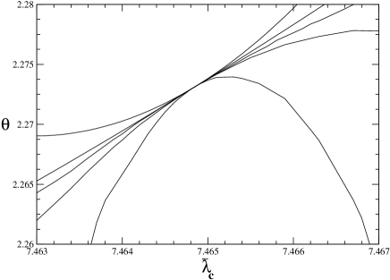
Figure 1: Biased estimates of $\theta=\nu_{\,||}(1+\eta)$ as a function of $\tilde{\lambda}_{c}$ derived from the Padé approximants to the series $(\lambda-\tilde{\lambda}_{c})(d/d\lambda)$ $\ln N=\theta$ evaluated at $\tilde{\lambda}_{c}$ for the PCCP. The approximants shown are [17/18], [18/17], [18,19], [19/18], and [18/18].

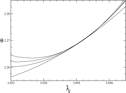
Figure 2: Biased estimates of $\theta=\nu_{\,||}(1+\eta)$ as a function of $\tilde{\lambda}_{c}$ derived from the Padé approximants to the series $(\lambda-\tilde{\lambda}_{c})(d/d\lambda)$ $\ln N=\theta$ evaluated at $\tilde{\lambda}_{c}$ for the APCCP. The approximants shown are [18/18], [17,18], [18/19], and [19/18].

From the Figs. 1, 2 and 3, we see a very narrow intersection of the Padé approximants, revealing the utility of this approach. However, as pointed out by Guttmann guttmann , it is difficult to estimate uncertainties in series calculations. Thus, in order to give a more realistic estimate of the quantities measured here and their associated uncertainties, we have estimated them by taking into account the first and last crossings among various Padé approximants. The values of the critical parameters obtained for the three models are summarized in the Table 3. The estimates of $\lambda_{c}$ for the PCCP and TCCP are in excellent agreement with the corresponding values $\lambda_{c}=7.464(2)$ and $\lambda_{c}=12.00(1)$ obtained from numerical simulations dictome ; fiore1 .

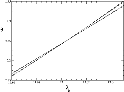
Figure 3: Biased estimates of $\theta=\nu_{\,||}(1+\eta)$ as a function of $\tilde{\lambda}_{c}$ derived from the Padé approximants to the series $(\lambda-\tilde{\lambda}_{c})(d/d\lambda)$ $\ln N=\theta$ evaluated at $\tilde{\lambda}_{c}$ for the TCCP. The approximants shown are [15/15], [15,16], [16,15], and [16,16].

Table 3: Biased estimates for $\lambda_{c}$ and $\nu_{\,||}(1+\eta)$ from the Padé approximants for the three models considered here together with the values for the basic contact process (CP) jen93b .

Model	$\lambda_{c}$	$\nu_{\,||}(1+\eta)$
PCCP	7.4650(6)	2.274(3)
APCCP	3.9553(5)	2.272(4)
TCCP	12.01(2)	2.26(2)
CP	3.29782	2.2772

Figure 4: Log-log plot of the number of particles $N_{s}$ versus the time $t$ for some values of $\lambda$ for the APCCP. From top to bottom $\lambda=3.97$, $3.9558$, $3.9553$, $3.95$, and $3.93$.

V Numerical simulation

As a check of the accuracy of the results obtained here, we have performed spreading simulations for the APCCP, since its critical point is unknown in the literature. Following Grassberger and de la Torre grassberger , we started from a initial configuration close to the absorbing state with only two adjacent particles, we can study the time evolution the survival probablility $P_{s}(t)$, the mean number of particles $N_{s}(t)$, and the mean-square distance of the particles from the origin $R(t)$. At the critical point, these quantities are governed by power-laws whose their related critical exponents are named $\delta$, $\eta$ and $z$, respectively. Off-critical point, we expect deviations from the power-law behavior. In the Fig. 4, we plotted the quantity $N_{s}(t)$ versus the time $t$ for some values of $\lambda$. Analogous analysis can be done for determing the exponents $\delta$ and $z$. At the critical value $\lambda_{c}=3.9553$, our data for the three quantities $N_{s}(t)$, $P_{s}(t)$, and $R(t)$ follow indeed a power law behavior, whose critical exponents are consistent with those of the DP universality class.

VI Conclusion

We have derived subcritical series expansions for studying the critical behavior of three nonequilibrium systems characterized by multiple-creation of particles. Although series expansion have been applied sucessfully for the contact process and similar models jen93b ; jen1993 ; jendic1994 , this is the first time that these systems, with multi-reaction rules, has been treated by means of a technique other than numerical simulations. With exception of the TCCP, whose value of $\lambda_{c}$ are in the same level of precision of numerical simulation estimates, the subcritical series expansion give us the best estimates for the critical point of the models considered here. The critical exponents are consistent with those related to models beloging in the DP universality class. We remark finally that the present approach may be very useful to determine the critical behavior and universality classes for other nonequilibrium systems.

References

- (1) T. E. Harris, Ann. Probab. 2, 969 (1974).
- (2) J. Marro and R. Dickman, Nonequilibrium Phase Transitions in Lattice Models (Cambridge University Press, Cambridge, 1999).
- (3) R. Dickman, Phys. Rev. E 50, 4404 (1994).
- (4) I. Dornic, H. Chaté, and M. A. Muñoz, Phys. Rev. Lett. 94, 100601 (2005).
- (5) J. Hooyberghs and C. Vanderzande, J. Phys. A 33, 907 (2000).
- (6) J. Hooyberghs and C. Vanderzande, Phys. Rev. E, 63, 041109 (2001).
- (7) R. Dickman, J. Stat. Phys. 55, 997 (1989).
- (8) I. Jensen and R. Dickman, J. Phys. A 26, L151 (1993).
- (9) I. Jensen and R. Dickman, Physica A 203, 175 (1994).
- (10) N. Inui and A. Yu. Tretyakov, Phys. Rev. Lett 80, 5148 (1998).
- (11) R. Dickman and T. Tomé, Phys. Rev. A 44, 4833 (1991).
- (12) C. E. Fiore and M. J. de Oliveira, Phys. Rev. E, 70, 046131 (2004).
- (13) T. Tomé and M. J. de Oliveira, Phys. Rev. E 72, 026130 (2005).
- (14) M. J. de Oliveira (unpublished).
- (15) Phase Transitions and Critical Phenomena, vol. 13, edited by C. Domb and J. L. Lebowitz (Academic Press, New York, 1989).
- (16) G. A. Baker, Quantitative Theory of Critical Phenomena, vol. 3, edited by C. Domb and J. L. Lebowitz (Academic Press, Boston, 1990).
- (17) I. Jensen and R. Dickman, J. Stat. Phys. 71, 89 (1993).
- (18) R. Dickman and I. Jensen, Phys. Rev. Lett 67, 2391 (1991).
- (19) W. G. Dantas and J. F. Stilck, J. Phys. A, 38, 5841 (2005).
- (20) P. Grassberger and A. de la Torre, Ann. Phys. (N.Y.) 122, 373 (1979).