Jahn-Teller distortions and phase separation in doped manganites

Abstract

A ”minimal model” of the Kondo-lattice type is used to describe a competition between the localization and metallicity in doped manganites and related magnetic oxides with Jahn-Teller ions. It is shown that the number of itinerant charge carriers can be significantly lower than that implied by the doping level $x$. A strong tendency to the phase separation is demonstrated for a wide range of intermediate doping concentrations vanishing at low and high doping. The phase diagram of the model in the $x-T$ plane is constructed. At low temperatures, the system is in a state with a long-range magnetic order: antiferromagnetic (AF), ferromagnetic (FM), or AF–FM phase separated (PS) state. At high temperatures, there can exist two types of the paramagnetic (PM) state with zero and nonzero density of the itinerant electrons. In the intermediate temperature range, the phase diagram includes different kinds of the PS states: AF–FM, FM–PM, and PM with different content of itinerant electrons. The applied magnetic field changes the phase diagram favoring the FM ordering. It is shown that the variation of temperature or magnetic field can induce the metal-insulator transition in a certain range of doping levels.

I Introduction

The effect of electron correlations on the properties of different materials is currently among the most burning problems of the condensed matter physics. As a rule, strong electron correlations are accompanied by the formation of nanoscale inhomogeneous states DagSci . Such inhomogeneities have been already studied for several decades. In particular, they were widely discussed for high-$T_{c}$ superconductors NagSup and heavy fermion materials fermion . In the recent years, they attract a special attention owing to the discovery of the colossal magnetoresistance effect in manganites (the nature of which is believed to be closely related to inhomogeneous structures dagbook ). The inhomogeneities manifest themselves in other magnetic materials such as cobaltites cobalt , nickelates nickel and also in low-dimensional magnets low-d . All these systems are characterized by a strong interplay of spin, charge, and orbital degrees of freedom leading to rather rich phase diagrams.

One of the first most spectacular examples of such kind of inhomogeneities is the formation of ferromagnetic (FM) droplets (magnetic polarons or ferrons) in antiferromagnetic (AF) semiconductors at low doping levels as well as FM spin polarons in the paramagnetic state Nag67 ; Kasuya . These examples correspond to the case of so called electron phase separation caused by self-trapping of charge carriers, which change their local environment. In addition to such a small-scale phase separation, in manganites, as well as in other compounds exhibiting first order transitions (e.g., between FM and AF phases), there also arises the phase separation of another type related to rather wide region where different phases coexist. An example of such large-scale phase separation is the formation of rather large FM droplets with the size of the order of (100-1000) $\AA$ inside the AF matrix Bala ; Ueh . At higher doping levels close to the half-filling, there appears one more threshold for the phase separation in the system corresponding again to the formation of ferromagnetic droplets, but now in a charge-ordered insulating matrix KKK . The interaction of spin, charge, and orbital degrees of freedom can also lead to the formation of stripe structures instead of droplets at high content of the alkaline-earth element stripes . In manganites, owing to the strong electron-lattice interactions, such structures are related to the lattice distortions and can be observed by the electron diffraction and the low-angle neutron scattering KuKh .

Both analytical and numerical studies in various models related to the strongly correlated electrons exhibit a pronounced tendency toward phase separation in a wide range of temperatures and electron or hole concentrations. Among these, we can mention $s-d$ Kak , $t-J$ t-J , Hubbard Viss , and Falicov-Kimball PSfal models.

The theoretical models usually imply that the number of charge carriers introduced by doping is equal to the number of itinerant electrons which take part in the formation of nanoscale inhomogeneities. However, the comparison of experimental data with the theoretical results suggests that such an approach is insufficient zhao and the number of self-trapped carriers can significantly differ from the doping level prbMi ; zhetf04 .

Here, we analyze the model proposed in our paper Ref. prlKRS, , which relates the doping level and the number of charge carriers. We take into account the Jahn-Teller (JT) nature of magnetic ions, which could give rise to the localization of charge carriers at the lattice distortions. We introduce this localization effect to the Kondo-lattice model in the double exchange limit. Beginning from seminal paper, Ref. Millis, , the role of JT distortions was widely discussed in literature dagbook ; hor ; bus . In particular, such distortions were taken into consideration in Refs. Rama, ; Rama1, in the analysis of the phase diagram of doped manganites. However, none of these papers dealt with the phase separation phenomena. In our paper, the main emphasis is made on the studying the phase diagram in the doping–temperature ($x-T$) plane and its evolution under effect of the applied magnetic field.

II The model

First, let us note that the doped manganites, (Re${}_{1-x}^{3+}$Mn${}_{1-x}^{3+}$)(A${}_{x}^{2+}$Mn${}_{x}^{4+}$)O${}_{3}^{2-}$, are the compounds with mixed valence. Here Re is a trivalent rare-earth element and A is a bivalent alkaline-earth element. The ions Mn³⁺ and Mn⁴⁺ have $3d^{4}$ and $3d^{3}$ electron configurations, respectively. In such compounds, manganese ions are located in the centers of O₆ octahedra. In a regular octahedron, a five-fold degenerate $3d$ level is split into triple- and double-degenerate levels, $t_{2g}$ ($d_{xy}$, $d_{yz}$, $d_{zx}$) and $e_{g}$ ($d_{x^{2}-y^{2}}$, $d_{3z^{2}-r^{2}}$), respectively. The $t_{2g}$ level lies lower than $e_{g}$ level. Manganese ions are characterized by the strong Hund’s rule coupling giving rise to the parallel alignment of intra-atomic electron spins. So, the spins of $t_{2g}$ electrons form local spin $S=3/2$. In a regular MnO₆ octahedron, Mn³⁺ ion has one electron at double-degenerate $e_{g}$ level Good . According to the Jahn-Teller theorem, the latter configuration is unstable and the degeneracy is lifted by a distortion of the octahedron. The Mn⁴⁺ is not a Jahn-Teller ion and Mn⁴⁺O₆ octahedron remains undistorted. The distortion of Mn³⁺O₆ octahedron leads to the energy lowering by $\epsilon_{JT}$. In doped manganites, the $e_{g}$ electron can hop from Mn³⁺ to Mn⁴⁺ ion producing a gain in the kinetic energy due to electron delocalization. Therefore, an electron can lower its energy either due to the Jahn-Teller-induced localization at distorted octahedra or by the delocalization related to the inter-atomic hopping. The strong Hund’s rule coupling favors the hopping of an electron when its spin is parallel to the spin of core ($t_{2g}$) electrons. This is the origin of the well-known double-exchange mechanism of ferromagnetic interaction between the localized spins Zener .

Therefore, it is natural to assume that the $e_{g}$ electron can be either localized due to Jahn-Teller distortions with the energy gain $\epsilon_{JT}$ ($l$ electron) or to decrease its energy due to band broadening ($b$ electron) Pai ; Rama ; Rama1 . So, there exists a competition between the localization and delocalization. Such a system with localized and band electrons can be analyzed using the Hubbard Hamiltonian taking into account the electron-lattice interaction, the Hund’s rule coupling, and the exchange interaction between core electrons prlKRS

$$\hat{H} = H_{\text{el}}+H_{\text{AF}}+H_{\text{JT}}+H_{\text{el-el}}\,,$$ (1)

$$H_{\text{el}} = -\sum_{\langle{\bf n}{\bf m}\rangle}\sum_{ab\sigma}\left(t^{ab}_{{\bf n}{\bf m}}a^{{\dagger}}_{{\bf n}a\sigma}a_{{\bf m}b\sigma}+h.c.\right)$$

$$-\frac{J_{H}}{2}\!\sum_{{\bf n}}\!\sum_{a\sigma\sigma^{\prime}}a^{{\dagger}}_{{\bf n}a\sigma}\left({\bm{\sigma}}{\bf S}_{{\bf n}}\right)_{\sigma\sigma^{\prime}}a_{{\bf n}a\sigma^{\prime}}\,,$$

$$H_{\text{AF}} = J^{\prime}\!\!\!\sum_{\langle{\bf n}{\bf m}\rangle}{\bf S}_{{\bf n}}{\bf S}_{{\bf m}},$$

$$H_{\text{JT}} = -g\sum_{{\bf n}}\sum_{ab\sigma}a^{{\dagger}}_{{\bf n}a\sigma}\left[Q_{2{\bf n}}(\sigma^{x})_{ab}+Q_{3{\bf n}}(\sigma^{z})_{ab}\right]a_{{\bf n}b\sigma}$$

$$+\frac{K}{2}\sum_{{\bf n}}\left(Q_{2{\bf n}}^{\,2}+Q_{3{\bf n}}^{\,2}\right)\,,$$

$$H_{\text{el-el}} = \frac{U_{1}}{2}\sum_{{\bf n}a\sigma}n_{{\bf n}a\sigma}n_{{\bf n}a\bar{\sigma}}+\frac{U_{2}}{2}\sum_{{\bf n}a\sigma\sigma^{\prime}}n_{{\bf n}a\sigma}n_{{\bf n}\bar{a}\sigma^{\prime}}\,.$$

In this Hamiltonian, $a^{{\dagger}}_{{\bf n}a\sigma}$, $a_{{\bf n}a\sigma}$ are creation and annihilation operators for $e_{g}$ electrons at site ${\bf n}$ with orbital index $a$ ($3z^{2}-r^{2}$ or $x^{2}-y^{2}$) and spin projection $\sigma$, ${\bf S_{n}}$ is a local spin of $t_{2g}$ electrons. Below we will consider ${\bf S_{n}}$ as classical vectors. $\bm{\sigma}$ are the Pauli matrices and $Q_{2{\bf n}}$, $Q_{3{\bf n}}$ are normal modes of vibration of MnO₆ octahedron. The symbol $\langle{\bf nm}\rangle$ denotes the summation over nearest sites. The electron part $H_{\text{el}}$ of Hamiltonian (1) includes the kinetic energy of $e_{g}$ electrons and the Hund’s rule coupling between the spins of $e_{g}$ and $t_{2g}$ electrons. $H_{\text{AF}}$ is the antiferromagnetic ($J^{\prime}>0$) exchange interaction between local spins. The $H_{\text{JT}}$ term takes into account interactions between $e_{g}$ electrons and vibrational modes for the MnO₆ octahedra, here $K$ is the elastic energy and $g$ is the electron-lattice coupling constant. The on-site Coulomb repulsion $H_{\text{el-el}}$ includes the terms corresponding to $e_{g}$ electrons at the same and different orbitals, where the bar above $a$ or $\sigma$ means not $a$ or not $\sigma$, respectively.

We consider the limit $J_{H}\to\infty$ characteristic of manganites. In this case, the spin of $e_{g}$ electrons is parallel to $\textbf{S}_{\bf{n}}$ and we can eliminate the spin indices by the transformation of $a_{{\bf n}a\sigma}$ to operators $c_{{\bf n}a}$ with spin projection $+1/2$ onto the direction of ${\bf S_{n}}$ accompanied by the transformation of hopping amplitudes degen : $t^{ab}_{{\bf n}{\bf m}}\to t^{ab}_{{\bf n}{\bf m}}\cos(\nu_{{\bf nm}}/2)$, where $\cos\nu_{{\bf nm}}={\bf S_{n}}{\bf S_{m}}/S^{2}$. In addition, we assume that $t^{(l)}_{{\bf n}{\bf m}}\to 0$ for $l$ electrons, which produce maximum splitting of $e_{g}$ level with the energy gain $-g^{2}/2K$, whereas $b$ electrons with non-zero hopping integrals $t^{(b)}_{{\bf n}{\bf m}}$ produce smaller distortions of MnO₆ octahedra. Preliminary calculations for the case $t^{(l)}_{{\bf n}{\bf m}}\neq 0$ demonstrated that the results are not significantly affected if the ’localized’ band is much narrower than itinerant one. Therefore, in this paper, we consider the limiting case of zero hopping integral for ’localized’ electrons. Hamiltonian then reads

$$H^{\prime}_{\text{eff}} = H_{\text{eff}}-\mu\sum_{{\bf n}}\left(n_{l{\bf n}}+n_{b{\bf n}}\right)\,,$$ (2)

$$H_{\text{eff}} = -t\sum_{\langle{\bf nm}\rangle}c^{{\dagger}}_{{\bf n}}c_{{\bf m}}\sqrt{\frac{S^{2}+\mathbf{S}_{\mathbf{n}}\mathbf{S}_{\mathbf{m}}}{2S^{2}}}-\epsilon_{\text{JT}}\sum_{{\bf n}}n_{l{\bf n}}$$

$$+U\sum_{{\bf n}}n_{l{\bf n}}n_{b{\bf n}}+J^{\prime}\sum_{{\langle{\bf nm}\rangle}}\mathbf{S}_{\mathbf{n}}\mathbf{S}_{\mathbf{m}}\,,$$

where $n_{b{\bf n}}=c^{{\dagger}}_{{\bf n}}c_{{\bf n}}$ and $n_{l{\bf n}}=l^{{\dagger}}_{{\bf n}}l_{{\bf n}}$ are the numbers of $b$ and $l$ electrons at site ${\bf n}$, $c^{{\dagger}}_{{\bf n}}$, $c_{{\bf n}}$ and $l^{{\dagger}}_{{\bf n}}$, $l_{{\bf n}}$ are the creation and annihilation operators for the $b$ and $l$ electrons, respectively, and $\mu$ is the chemical potential. The first three terms in $H_{\text{eff}}$ correspond, respectively, to the kinetic energy of $b$ electrons, JT energy of localized electrons, and on-site Coulomb repulsion between $b$ and $l$ electrons. The last term in $H_{\text{eff}}$ is the Heisenberg antiferromagnetic exchange between local spins. The effective on-site Coulomb repulsion $U$ in Eq. (2) can differ from $U_{2}$, but has the same order of magnitude ($\sim 5\,eV$). $\epsilon_{\text{JT}}\sim g^{2}/2K$ is the JT energy gain for $l$ electrons counting from the center of $b$ electron band. The number of localized, $n_{l}$, and band, $n_{b}$, electrons per lattice site obeys an obvious relation $n_{b}+n_{l}=1-x$, where $x$ is the doping level.

In our paper, we limit ourselves by the case of the large on-site Coulomb repulsion $U$, which strongly suppresses double occupancy of the site. Moreover, at large $U$, the characteristic time of existence for a ’double electron state’ is of the order of $1/U\ll 1/\Omega$, where $\Omega$ is the characteristic JT phonon frequency ($\hbar=1$), which is of the order of Debye frequency. Therefore, the adiabatic approximation for the Jahn-Teller distortions is applicable. As a result, the JT term in Eq. (2) is determined only by localized electrons.

Hamiltonian (2) was analyzed at zero temperature in Ref. prlKRS, . The homogenous ferromagnetic and antiferromagnetic states as well as the phase-separated FM-AF state were studied. The effective parameters $t$ and $\epsilon_{\text{JT}}$ were considered to be independent of the densities of band $n_{b}$ and localized $n_{l}$ electrons. In the present analysis, we also neglect the dependence of parameters $\epsilon_{\text{JT}}$ and $t$ on $n_{b}$ and $n_{l}$, but take into account the temperature dependence of hopping integral $t$, which can be rather strong due to polaron band narrowing polaron ; KH . Following Refs. polaron, ; KH, we write the expression for the hopping integral in the form

$$t(T)=t_{0}\exp\left(-\frac{2\lambda^{2}}{\text{e}^{\Omega/T}-1}\right)\,.$$ (3)

In this expression, $\lambda$ is the dimensionless electron-phonon coupling constant. From Eq. (3), it is clear that the hopping integral $t(T)$ decreases with temperature. Even if we take into account the finite bandwidth for ’localized’ electrons, it will also decrease with $T$. However, the parameters describing this behavior could be different for different bands. We cannot assert that at high temperatures the ratio of widths for the narrow and wide bands would be larger or smaller than at low temperatures. In this paper, we consider the temperature range, which is relatively small as compared to characteristic value of $\Omega$. Thus, $t(T)$ does not vary by orders of magnitude and the bandwidth ratio remains small.

To study the effects of temperature, we use the mean field (MF) approximation. For this purpose, we make a decoupling procedure in the first term of $H_{\text{eff}}$, Eq. (2), in the following way. The values of $c^{{\dagger}}_{{\bf n}}c_{{\bf m}}$ and $\vartheta_{\bf nm}\equiv\sqrt{(S^{2}+\mathbf{S}_{\mathbf{n}}\mathbf{S}_{\mathbf{m}})/2S^{2}}=\sqrt{(1+\mathbf{e}_{\mathbf{n}}\mathbf{e}_{\mathbf{m}})/2}$ can be written as

$$c^{{\dagger}}_{{\bf n}}c_{{\bf m}}=\left\langle c^{{\dagger}}_{{\bf n}}c_{{\bf m}}\right\rangle+\delta\left(c^{{\dagger}}_{{\bf n}}c_{{\bf m}}\right),\,\,\vartheta_{\bf nm}=\left\langle\vartheta_{\bf nm}\right\rangle+\delta\vartheta_{\bf nm}\,,$$

where angular brackets mean thermal averaging, $\mathbf{S}_{\mathbf{n}}=S\mathbf{e}_{\mathbf{n}}$, and $\mathbf{e}_{\mathbf{n}}$ is the unit vector. Omitting the products proportional to $\delta\left(c^{{\dagger}}_{{\bf n}}c_{{\bf m}}\right)\delta\vartheta_{\bf nm}$, we write the first term in $H_{\text{eff}}$ as

$$-\bar{t}\sum_{\langle{\bf nm}\rangle}c^{{\dagger}}_{{\bf n}}c_{{\bf m}}-\sum_{\langle{\bf nm}\rangle}\left\langle c^{{\dagger}}_{{\bf n}}c_{{\bf m}}\right\rangle\left(t\sqrt{\frac{1+\mathbf{e}_{\mathbf{n}}\mathbf{e}_{\mathbf{m}}}{2}}-\bar{t}\right)\,,$$

where $\bar{t}=t(T)\left\langle\sqrt{(1+\mathbf{e}_{\mathbf{n}}\mathbf{e}_{\mathbf{m}})/2}\right\rangle$. Note that in homogenous state, $\left\langle\vartheta_{\bf nm}\right\rangle$ does not depend on indices ${\bf n}$ and ${\bf m}$ (for sites $\mathbf{m}$ nearest to the site $\mathbf{n}$). Now, the effective Hamiltonian can be represented as a sum of electronic and magnetic parts

$$H^{MF}_{\text{eff}}=H_{\text{el}}+H_{\text{m}}-\mu\sum_{\bf{n}}(n_{l\bf{n}}+n_{b\bf{n}})\,,$$

$$H_{\text{el}}=-\bar{t}\sum_{\langle{\bf nm}\rangle}c^{{\dagger}}_{{\bf n}}c_{{\bf m}}-\epsilon_{\text{JT}}\sum_{{\bf n}}n_{l{\bf n}}+U\sum_{{\bf n}}n_{l{\bf n}}n_{b{\bf n}},$$ (4)

$$H_{\text{m}}=-\sum_{\langle{\bf nm}\rangle}\left[\left\langle c^{{\dagger}}_{{\bf n}}c_{{\bf m}}\right\rangle\left(t\vartheta_{\bf nm}-\bar{t}\right)-J^{\prime}S^{2}\mathbf{e_{n}}\mathbf{e_{m}}\right].$$ (5)

III Homogeneous states

III.1 Ferromagnetic state

In the ferromagnetic state, we have $\langle\mathbf{e_{n}e_{m}}\rangle=1$ far below the Curie temperature. First, we consider the electronic sector of the problem. The Hamiltonian $H_{\text{el}}$ is similar to that considered in Ref. prlKRS, and the temperature $T$ enters only the effective hopping integral $\bar{t}(T)$. To calculate the free energy of the electronic subsystem, we use the Hubbard I decoupling for the one-$b$-electron Green function $G_{b}({\bf n,n}_{0};\,\tau-\tau_{0})=-i\langle\langle\hat{T}c_{{\bf n}}(\tau)c^{{\dagger}}_{{\bf n}_{0}}(\tau_{0})\rangle\rangle$, as in Ref. prlKRS, . Here $\tau$ is the time variable and $\hat{T}$ is the time-ordering operator. The equation of motion for $G_{b}({\bf n,n}_{0};\,\tau-\tau_{0})$ can be written in the form:

$$\left(i\frac{\partial}{\partial\tau}+\mu\right)G_{b}({\bf n,n}_{0};\,\tau-\tau_{0})=\delta_{{\bf nn}_{0}}\delta(\tau-\tau_{0})$$

$$-\bar{t}\sum_{{\bf\Delta}}G_{b}({\bf n}+{\bf\Delta,n}_{0};\,\tau-\tau_{0})+U{\cal{G}}({\bf n,n}_{0};\,\tau-\tau_{0})\,,$$ (6)

where summation is performed over sites nearest to site ${\bf n}$, and ${\cal{G}}$ is the ’two-particle’ Green function ${\cal{G}}({\bf n,n}_{0};\,\tau-\tau_{0})=-i\langle\langle\hat{T}c_{{\bf n}}(\tau)n_{l{\bf n}}(\tau)c^{{\dagger}}_{{\bf n}_{0}}(\tau_{0})\rangle\rangle$. The equation of motion for ${\cal{G}}$ is

$$\left(i\frac{\partial}{\partial\tau}+\mu-U\right){\cal{G}}({\bf n,n}_{0};\,\tau-\tau_{0})=n_{l}\delta_{{\bf nn}_{0}}\delta(\tau-\tau_{0})$$

$$+i\bar{t}\sum_{{\bf\Delta}}\left\{\langle\langle\hat{T}n_{l{\bf n}}(\tau)c_{{\bf n}+{\bf\Delta}}(\tau)c^{{\dagger}}_{{\bf n}_{0}}(\tau_{0})\rangle\rangle\right.$$

$$+\langle\langle\hat{T}l^{{\dagger}}_{{\bf n}}(\tau)l_{{\bf n}+{\bf\Delta}}(\tau)c_{{\bf n}}(\tau)c^{{\dagger}}_{{\bf n}_{0}}(\tau_{0})\rangle\rangle$$

$$\left.-\langle\langle\hat{T}l^{{\dagger}}_{{\bf n}-{\bf\Delta}}(\tau)l_{{\bf n}}(\tau)c_{{\bf n}}(\tau)c^{{\dagger}}_{{\bf n}_{0}}(\tau_{0})\rangle\rangle\right\}\,.$$ (7)

The decoupling in the first term in curly brackets gives $\langle\langle n_{l{\bf n}}(\tau)\rangle\rangle\langle\langle\hat{T}c_{{\bf n}+{\bf\Delta}}(\tau)c^{{\dagger}}_{{\bf n}_{0}}(\tau_{0})\rangle\rangle=in_{l}G_{b}({\bf n}+{\bf\Delta},{\bf n}_{0};\,\tau-\tau_{0})$. Making similar decoupling in the next two terms, we get

$$iG_{b}({\bf n,n}_{0};\,\tau-\tau_{0})$$

$$\times\sum\limits_{\bf\Delta}\left\{\langle\langle l^{{\dagger}}_{{\bf n}}(\tau)l_{{\bf n}+{\bf\Delta}}(\tau)\rangle\rangle\right. \left.-\langle\langle l^{{\dagger}}_{{\bf n}-{\bf\Delta}}(\tau)l_{{\bf n}}(\tau)\rangle\rangle\right\}.$$

In the homogeneous ferromagnetic state, the sum evidently vanishes. As a result, we obtain the closed system of equations for $G_{b}$ and ${\cal{G}}$. In the frequency-momentum representation, the solutions for $G_{b}$ and ${\cal{G}}$ are as follows

$$\left\{\begin{array}[]{rcl}G_{b}({\bf k},\omega)&=&\displaystyle\frac{\omega+\mu-U(1-n_{l})}{E_{2}({\bf k})-E_{1}({\bf k})}\\ &\times&\left(\displaystyle\frac{1}{\omega+\mu-E_{2}({\bf k})}-\frac{1}{\omega+\mu-E_{1}({\bf k})}\right)\,,\\ &&\\ {\cal{G}}({\bf k},\omega)&=&n_{l}\displaystyle\frac{1+\bar{w}\zeta({\bf k})G_{b}({\bf k},\omega)}{\omega+\mu-U}\,,\end{array}\right.$$ (8)

where

$$E_{1,2}({\bf k})=\frac{U+\bar{w}\zeta({\bf k})}{2}\mp\sqrt{\left(\frac{U-\bar{w}\zeta({\bf k})}{2}\right)^{2}+U\bar{w}\zeta({\bf k})n_{l}}\,.$$ (9)

In these expressions,

$$\bar{w}=zt_{0}\exp\left(-\frac{2\lambda^{2}}{\text{e}^{\hbar\Omega/T}-1}\right)\left\langle\sqrt{\frac{1+\mathbf{e_{0}e_{\Delta}}}{2}}\right\rangle\,,$$ (10)

and

$$\zeta({\bf k})=-\frac{1}{z}\sum_{\mathbf{\Delta}}\text{e}^{i\mathbf{k\Delta}}\,,$$

where $z$ is the number of nearest neighbors. In the case of the simple cubic lattice, we have $z=6$ and in the tight-binding approximation

$$\zeta({\bf k})=-\frac{1}{3}\left[\cos(k^{1}d)+\cos(k^{2}d)+\cos(k^{3}d)\right],$$ (11)

where $d$ is the lattice constant and $k^{i}$ are the components of the wave vector.

From Eq. (8), it follows that the energy spectrum of $b$ electrons includes two sub-bands given by Eq. (9) and the number of states in each sub-band depends on $n_{l}$. In the limit of large $U$, which is relevant to magnetic oxides, Eq. (9) can be written as

$$E_{1}=\bar{w}\zeta({\bf k})(1-n_{l}),\,\,\,E_{2}=U+\bar{w}\zeta({\bf k})n_{l}.$$ (12)

It is clear from Eq. (12) that the width of the lower sub-band is $W=2(1-n_{l})\bar{w}$ while the width of the upper sub-band is $2n_{l}\bar{w}$. The total number of states in two sub-bands per site is equal to one and the number of states in the lower and upper sub-bands is equal to $1-n_{l}$ and $n_{l}$, respectively. Note that this result is valid for any value of $U$ as it can be demonstrated by integration of the corresponding terms in the Green function Eq. (8). Thus, at any doping level $x$ and temperature $T\ll U$ the upper sub-band is empty since $n_{b}+n_{l}=n=1-x$. In this case, it is reasonable to use the $U\to\infty$ limit. The Green function $G_{b}$ then becomes

$$G_{b}({\bf k},\omega)=\frac{1-n_{l}}{\omega+\mu-(1-n_{l})\bar{w}\zeta(\mathbf{k})}\,.$$ (13)

At low temperatures, $T\ll\bar{w}$, it is reasonable to represenr the Fermi-Dirac distribution function for $b$ electrons $f(E)=[\exp\{(E-\mu)/T\}+1]^{-1}$ by the step function $\theta(\mu-E)$. It can be shown that this approximation works well at $t,\epsilon_{\text{JT}}\gg J$, and $T\lesssim J$, where $J=zJ^{\prime}S^{2}$. An appreciable discrepancy could arise only at doping levels $x\ll 1$ and $1-x\ll 1$. However, at these doping levels, the homogeneous ferromagnetic state is unfavorable (see below). Therefore, the number of $b$ electrons can be expressed through the Green function as

$$n_{b}=-i\int\frac{d\omega}{2\pi}\int\frac{d^{3}k}{(2\pi)^{3}}\,G_{b}({\bf k},\omega+i0\!\cdot\!\text{sgn}\,\omega)\text{e}^{i\omega 0}\,.$$ (14)

This relationship defines $n_{b}$ as a function of chemical potential $\mu$ and $n_{l}$. The value of $n_{l}$ depends on relative positions of $\mu$ and $\epsilon_{JT}$.

If $\mu<-\epsilon_{\text{JT}}$, then the Jahn-Teller-induced localization is unfavorable, $n_{l}=0$, $n_{b}=1-x$, and the chemical potential is found from Eq. (14). With the increase of $n_{b}$, $\mu$ becomes equal to $-\epsilon_{JT}$, the further growth in the number of itinerant charge carriers is ceased, $n_{l}$ becomes nonzero, and $\mu$ is pinned at the level $-\epsilon_{JT}$. In the latter case, the number of localized electrons can be found from Eq. (14) at $\mu=-\epsilon_{JT}$ using the relation $n_{b}=1-x-n_{l}$. As a result, we get

$$(1-n_{l})\left[1-n_{0}\left(-\frac{\epsilon_{JT}}{\bar{w}(1-n_{l})}\right)\right]=x\,,$$ (15)

where

$$n_{0}(\mu^{\prime})=\int\limits_{-1}^{\mu^{\prime}}dE^{\prime}\,\rho_{0}(E^{\prime})\,,$$ (16)

and

$$\rho_{0}(E^{\prime})=\displaystyle\int\frac{d^{3}\mathbf{k}}{(2\pi)^{3}}\,\delta(E^{\prime}-\zeta(\mathbf{k}))$$ (17)

is the density of states of free electrons.

At zero doping, $x=0$, the number of localized electrons $n_{l}=1$, and the bandwidth $W=0$. At low doping, all electrons are localized, $n_{l}=1-x$ and $W=2x\bar{w}$, until the bottom of the band reaches the energy of $l$ electrons $-\epsilon_{\text{JT}}$ at some critical concentration $x=x_{1}(T)=\epsilon_{\text{JT}}/\bar{w}$. At $x>x_{1}(T)$ the localized and band electrons coexist as long as $x$ is smaller than the second critical doping level $x_{2}(T)$ at which the existence of localized electrons becomes unfavorable, that is, $n_{l}=0$ if $x>x_{2}(T)$. From Eq. (15) we find $x_{2}(T)=1-n_{0}(-\epsilon_{\text{JT}}/\bar{w})$. Naturally, such a picture can exist only for a certain relationship between the parameters of the model, in particular, if $\epsilon_{\text{JT}}<\bar{w}$. Since $\bar{w}$ decreases with the growth of temperature, both these critical concentrations, $x_{1}$ and $x_{2}$, become larger when temperature increases. Note that the homogeneous ferromagnetic state can exist only at $x>x_{1}$ if $n_{b}\neq 0$.

Figure 1: The dependence of $n_{l}$ (solid line) and $n_{b}$ (dashed line) on doping concentration $x$ at $\epsilon_{JT}/\bar{w}=0.05$.

The values of $n_{l}$ and $n_{b}$ as the functions of doping $x$ are shown in Fig. 1 at typical parameters of the model. These calculations and calculations below are performed for a simple cubic lattice with $\zeta({\bf k})$ given by Eq. (11). In this case, the expressions for $\rho_{0}(E^{\prime})$ and $n_{0}(\mu^{\prime})$ in Eqs. (17) and (16) are found in Appendix A, see Eqs. (50) and (51), respectively.

At $x_{1}(T)<x<x_{2}(T)$, the kinetic energy of $b$ electrons per site can be written as

$$E_{\text{kin}} = -\bar{t}\sum_{\Delta}\langle c^{{\dagger}}_{\bf 0}c_{{\bf\Delta}}\rangle$$

$$= -i\bar{w}\!\!\int\frac{d\omega}{2\pi}\int\!\!\frac{d^{3}k}{(2\pi)^{3}}\,\zeta(\mathbf{k})G_{b}({\bf k},\omega+i0\!\cdot\!\text{sgn}\,\omega)\text{e}^{i\omega 0}$$

For further purposes we introduce the function

$$A(\epsilon^{\prime})=\frac{1}{z}\sum_{\Delta}\langle c^{{\dagger}}_{\bf 0}c_{{\bf\Delta}}\rangle=-(1-n_{l})\varepsilon_{0}\left(-\frac{\epsilon^{\prime}}{1-n_{l}}\right)\,,$$ (19)

where

$$\varepsilon_{0}(\mu^{\prime})=\int\limits_{-1}^{\mu^{\prime}}dE^{\prime}\,E^{\prime}\rho_{0}(E^{\prime})\,.$$ (20)

The kinetic energy of $b$ electrons then reads

$$E_{\text{kin}}=-\bar{w}A\left(\frac{\epsilon_{JT}}{\bar{w}}\right)\,.$$ (21)

The energy of the on-site Coulomb repulsion can be found using the ’two-particle’ Green function ${\cal{G}}$

$$U\langle n_{b0}n_{l0}\rangle=-iU\int\frac{d\omega}{2\pi}\int\frac{d^{3}k}{(2\pi)^{3}}\,{\cal{G}}({\bf k},\omega+i0\!\cdot\!\text{sgn}\,\omega)\text{e}^{i\omega 0}\,.$$ (22)

Since $\mu<U$, the pole coming from the denominator of the function ${\cal{G}}$ (see second Eq. (8)) does not contribute to the integral over $\omega$, and in the limit $U\to\infty$, we get

$$U\langle n_{b0}n_{l0}\rangle=n_{l}\,\bar{w}A\left(\frac{\epsilon_{JT}}{\bar{w}}\right)\,.$$ (23)

Note that we replace the Fermi-Dirac distribution by the step function. Therefore, we can omit the electron entropy term and write the free energy of electrons per site as a sum of Eqs. (21), (23), and the JT term

$$F_{\text{el}}=-(1-n_{l})\bar{w}A\left(\frac{\epsilon_{JT}}{\bar{w}}\right)-\epsilon_{JT}n_{l}\,.$$ (24)

For $x>x_{2}(T)$ when $n_{l}=0$, we should replace $\epsilon_{JT}/\bar{w}$ by $-\mu^{\prime}$ in formulas (21), (23), and (24), where $\mu^{\prime}$ is found from the equation $1-x=n_{0}(\mu^{\prime})$.

Now, we consider the magnetic part of the Hamiltonian, $H_{\text{m}}$, Eq. (5). Following the conventional mean field approach for spin systems Smart , we replace $\mathbf{e_{m}}=\{\sin\theta_{\mathbf{m}}\cos\phi_{\mathbf{m}},\,\sin\theta_{\mathbf{m}}\sin\phi_{\mathbf{m}},\,\cos\theta_{\mathbf{m}}\}$ in Eq. (5) by its mean value $\{0,\,0,\,m\}$, where $m=\langle\cos\theta_{\mathbf{m}}\rangle$. As a result, $H_{\text{m}}$ decouples into the sum of $N$ independent one-site Hamiltonians, $H_{\text{m}}=NH_{m0}$, where

$$H_{m0}(\cos\theta) = -A\left(\frac{\epsilon_{JT}}{\bar{w}}\right)\left(w(T)\sqrt{\frac{1+m\cos\theta}{2}}-\bar{w}\right)$$ (25)

$$+Jm\cos\theta\,,$$

$w(T)=zt(T)$. The value of $m$ is determined by the self-consistency condition

$$m=\displaystyle\frac{\int\limits_{-1}^{1}du\,u\text{e}^{-\beta H_{m0}(u)}}{\int\limits_{-1}^{1}du\,\text{e}^{-\beta H_{m0}(u)}}\,,$$ (26)

where $\beta=1/T$. We should also take into account that $\bar{w}$ is related to $H_{m0}(u)$ and $m$ by Eq.(10)

$$\bar{w}=\frac{w(T)}{\sqrt{2}}\displaystyle\frac{\int\limits_{-1}^{1}du\sqrt{1+um}\,\text{e}^{-\beta H_{m0}(u)}}{\int\limits_{-1}^{1}du\,\text{e}^{-\beta H_{m0}(u)}}\,.$$ (27)

In order to find the Curie temperature $T_{c}$, we expand right hand side of Eq. (26) in a power series in $m$. Using Eqs. (25) and (27) we find

$$m=a_{1}(T)\beta m-a_{3}(T)\beta m^{3}-a_{5}(T)\beta m^{5}+\dots\,.$$

The Curie temperature is found then from the condition

$$a_{1}(T_{C})=\frac{1}{3}\left[\frac{w(T_{C})}{2\sqrt{2}}A\left(\frac{\epsilon_{JT}\sqrt{2}}{w(T_{C})}\right)-J\right]=T_{C}\,.$$ (28)

If we neglect the effect of polaron band narrowing, $\lambda=0$, we find the explicit expression for the Curie temperature $T_{C}=[w_{0}A(\epsilon_{JT}\sqrt{2}/w_{0})/(2\sqrt{2})-J]/3$. It is clear that polaron band narrowing reduces $T_{C}$.

Let us now analyze the order of the phase transition at $T=T_{C}$, which depends on the sign of $a_{3}(T_{C})$, see Ref. Landau, . If $a_{3}(T_{C})>0$, then $m$ tends to zero at $T\to T_{C}$ as

$$m(T)\approx\sqrt{\frac{a_{1}(T)-T}{a_{3}(T)}}\,.$$ (29)

In this case, we have second order magnetic phase transition. In the opposite case $a_{3}(T_{C})<0$, $m$ behaves approximately as ($a_{5}(T)>0$)

$$m(T)\approx\left.\sqrt{\frac{|a_{3}(T)|}{a_{5}(T)}+\frac{a_{1}(T)-T}{a_{3}(T)}}\right|_{T\to T_{C}}\!\!\!\!\!\!\!\!\!\!\!\!\longrightarrow\sqrt{\frac{|a_{3}(T_{C})|}{a_{5}(T_{C})}}\neq 0,$$ (30)

and the transition to paramagnetic (PM) state is of the first order. The analysis shows that $a_{5}(T)>0$ for any values of parameters of the model, but the sign of $a_{3}(T_{C})$ can be both positive or negative depending on the doping level $x$. At some $x=x_{12}$, the coefficient $a_{3}(T_{C})$ changes its sign. At low doping, $x<x_{12}$, we have $a_{3}(T_{C})<0$ and the transition from the FM to PM state is of the first order. At $x>x_{12}$, we have the second order phase transition.

The free energy of the system per site is equal to

$$F_{\text{fm}}=F_{\text{el}}-T\ln Z_{m},\,\,Z_{m}=\left(S+\frac{1}{2}\right)\!\int\limits_{-1}^{1}du\,\text{e}^{-\beta H_{m0}(u)}.$$ (31)

At $T\to 0$, $m\to 1$, $\bar{w}\to w_{0}=zt_{0}$, $Z_{m}\approx\exp(-\beta J)$, and the free energy

$$\left.F_{\text{fm}}\right|_{T\to 0}\rightarrow-(1-n_{l})w_{0}A\left(\frac{\epsilon_{JT}}{w_{0}}\right)-\epsilon_{JT}n_{l}+J\,.$$

In the PM state, we have $m=0$, $\bar{w}=w(T)/\sqrt{2}$, $Z_{m}=2S+1$, and

$$F_{\text{pm}}=-(1-n_{l})\frac{w(T)}{\sqrt{2}}A\left(\frac{\epsilon_{JT}\sqrt{2}}{w(T)}\right)-\epsilon_{JT}n_{l}-T\ln(2S+1)\,.$$

The transition from FM to PM state does not mean that $n_{b}$ becomes zero. As it was mentioned above, $n_{b}\neq 0$ at $x>x_{1}(T)$ and the value of $x_{1}$ increases with the temperature. At a certain temperature $T^{*}$, $x_{1}(T)$ exceeds $x$. It is clear that $T^{*}>T_{C}$ since the FM state can exist only at $n_{b}\neq 0$. Therefore, in our model, in addition to magnetic phase transitions, there should exist an electronic transition to the state without itinerant electrons. The temperature $T^{*}$ is determined by the evident condition $x_{1}(T^{*})=\epsilon_{JT}\sqrt{2}/w(T^{*})=x$.

III.2 Antiferromagnetic and canted states

In our model, there can exist other homogeneous states competing with FM and PM states. It is natural to consider the two-sublattice antiferromagnetic and canted states. In the canted state, the angle $\nu$ (canting angle) between the local spins belonging to two sublattices varies from $\pi$ (AF state) to $0$ (FM state). Here we consider AF and canting states of $G$ type, that is, in the cubic lattice each site of one sublattice is surrounded by sites of the second sublattice.

At finite temperatures, the canting angle is defined as $\cos\nu=\langle\mathbf{e_{0}e_{\Delta}}\rangle$. In the mean field approximation used above, we have $\langle\mathbf{e_{0}e_{\Delta}}\rangle=\langle\mathbf{e_{0}}\rangle\langle\mathbf{e_{\Delta}}\rangle$. Thus, we can define variable $m$ similar to that introduced in the previous subsection, $m^{2}=\cos\nu$ if $\nu<\pi/2$ or $m^{2}=-\cos\nu$ if $\nu>\pi/2$. In the first case, the value of $m(T)$ and the free energy of the system is found in the same way as for FM state from Eqs. (25)–(27). The only difference is that $m=1$ at $T=0$ in FM state (or $\nu=0$) while $m(0)<1$ (or $\nu\neq 0$) in the canted state. Note that the temperature of the transition from canted to paramagnetic state, $T_{cant}$, is given by Eq. (28), where $T_{C}$ should be replaced by $T_{cant}$.

In the case $\cos\nu<0$, instead of Eq. (26) and (27), we have

$$-m=\displaystyle\frac{\int\limits_{-1}^{1}du\,u\text{e}^{-\beta H_{m0}(u)}}{\int\limits_{-1}^{1}du\,\text{e}^{-\beta H_{m0}(u)}}\,,$$ (32)

$$\bar{w}=\frac{w(T)}{\sqrt{2}}\displaystyle\frac{\int\limits_{-1}^{1}du\sqrt{1-um}\,\text{e}^{-\beta H_{m0}(u)}}{\int\limits_{-1}^{1}du\,\text{e}^{-\beta H_{m0}(u)}}\,,$$ (33)

where mean-field Hamiltonian $H_{m0}(u)$ is given by Eq. (25). The temperature of the phase transition from canting to PM state is found now from the equation

$$\frac{1}{3}\left[J-\frac{w(T_{cant})}{2\sqrt{2}}A\left(\frac{\epsilon_{JT}\sqrt{2}}{w(T_{cant})}\right)\right]=T_{cant}\,.$$ (34)

The canted state can exist at $n_{b}\neq 0$ since it arises in our model due to the motion of conduction electrons.

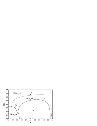
Figure 2: The phase diagram of the system without taking into account the possibility of phase separation. The regions $1$ and $2$ correspond to the canted states with $\cos\nu>0$ and $\cos\nu<0$, respectively. The parameters are $\epsilon_{JT}/w_{0}=0.05$, $J/w_{0}=0.01$, $\lambda=10$, and $\Omega/w_{0}=0.03$.

At doping levels $x<x_{1}(T)$, we have $n_{b}=0$ and the AF ordering is favorable. At rather low doping, $x<x_{1}(0)$, $n_{b}=0$ at any temperature. In this case, the Néel temperature is independent of $x$ and is determined by Eq. (34) as $T^{0}_{N}=J/3$. At higher doping, there can occur a transition from the AF state to the PM state with $n_{b}\neq 0$, and the Néel temperature, $T_{N}$, is determined by the comparison of free energies of corresponding states. In this doping range, the AF state turns out to be more favorable than the canted state. With the further increase of $x$, the phase with $n_{b}\neq 0$ has the lower energy, but this phase is FM rather than canted. The temperature of the AF–FM transition is found from the comparison of corresponding free energies. This transition is of the first order. Note that the phase diagram exhibits AF–FM–PM triple point at $x=x_{3}$ ($x_{3}<x_{12}$). The canted state can exist in the doping range $1-x\ll 1$, where the number of itinerant electrons is too small to stabilize the FM state. The corresponding phase diagram in the $x-T$ plane is shown in Fig. 2. We see that the competition between the itinerant and localized electrons gives rise to a rather complicated magnetic phase diagram of the system.

IV Phase separation

Up to this point, we considered only homogeneous states, however, it is well known that different inhomogeneous states are possible in the systems with strongly correlated electrons. So, we should compare the free energies of the states studied in the previous sections with those for inhomogeneous states. As a typical example of an inhomogeneous state, we analyze here the droplet model of electronic phase separation widely discussed in connection with manganites and other magnetic oxides. Among the possible types of phase separation, we treat below the coexistence of different phases: AF–FM, FM–PM, and PM phases with different values of $n_{b}$. For simplicity, we do not include into consideration the phase separation involving the canted state since it exists only in the narrow doping range. Note that our model always leads to such kind of phase separation, where we have $n_{b}=0$ in one of the phases.

We consider a system separated into two phases with the volume concentrations $p$ and $1-p$. In the homogeneous phases, the electron concentration per site coincides with the doping level $x$. In the inhomogeneous states, the electrons can be redistributed between the regions with different phases. Let $n_{b}\neq 0$ in the first (F) phase and $n_{b}=0$ in the second (A) phase, the electron density per site in the first phase is $x_{f}$ and in the second phase is $x_{a}$. So, doping level $x$ lies between $x_{a}$ and $x_{f}$. The charge conservation requires $p\,x_{f}+(1-p)x_{a}=x$.

In Fig. 3, we show the dependence of the free energy of the most favorable homogeneous state $F_{\text{hom}}=\min\left(F_{\text{fm}},F_{\text{af}},F_{\text{pm}},F_{\text{cant}}\right)$ on the doping level at different temperatures. The $F_{\text{hom}}(x)$ curves have two minima: one at $x=0$ and another near $x=x_{2}(T)$. Then we could expect that $x_{a}$ should be around zero, while $x_{f}$ should be close to $x=x_{2}(T)$.

The phase separation corresponds to the non-uniform charge density and we should take into account the Coulomb contribution to the total energy. This contribution depends on the structure of inhomogeneous state. To evaluate the Coulomb energy, we assume the spherical geometry of the phase-separated state. Namely, at $p<0.5$, the sample is modelled as an aggregate of spheres of F phase embedded into A matrix or that of A spheres in F phase for $p>0.5$. For this geometry, it is reasonable to calculate the Coulomb energy using the Wigner-Seitz approximation: each F or A sphere of radius $R_{s}$ is surrounded by a spherical cell of radius $R_{cell}$, such as the volume of the cell is $4\pi R_{cell}^{3}/3=V/N_{s}$, where $V$ is the volume of the sample and $N_{s}$ is the number of spheres. The radius $R_{cell}$ is related to $R_{s}$ as $R_{s}=p^{1/3}R_{cell}$ for $p<0.5$, and $R_{s}=(1-p)^{1/3}R_{cell}$ for $p>0.5$. The total electric charge inside this cell is zero and the Coulomb energy of the system is the sum of the electrostatic energies of these cells. Following Ref. Lor, , we obtain the expression for the Coulomb energy per site $E_{c}$ at $p<0.5$

$$E_{c}=\frac{2\pi e^{2}}{5\epsilon d}\,\left(x_{f}-x_{a}\right)^{2}\left(\frac{R_{s}}{d}\right)^{2}p\left(2-3p^{1/3}+p\right)\,,$$ (35)

where $\epsilon$ is the average permittivity of the sample and $d$ is the lattice constant. In the case $p>0.5$, we should replace $x_{f}\leftrightarrow x_{a}$ and $p\to 1-p$.

The $b$ electrons in the phase-separated state are confined within a restricted volume. The corresponding size quantization gives rise to the change in the density of states. The additional contribution to the energy (per site) is proportional to the total surface area between F and A phases, and at $p<0.5$ can be written in the form

$$E_{s}=p\,\frac{3d}{R_{s}}\sigma(x_{f})\,,$$ (36)

where surface energy $\sigma(x_{f})$ is calculated in Appendix A. In the case $p>0.5$, we should change $p\to 1-p$.

Figure 3: Free energy of homogeneous state $F_{\text{hom}}=\min(F_{\text{fm}},\,F_{\text{af}},\,F_{\text{pm}},\,F_{\text{cant}})$ vs. doping level $x$, at different temperatures. The dot curve corresponds to the function $x_{2}(T)$. The parameters are $\epsilon_{JT}/w_{0}=0.05$, $J/w_{0}=0.01$, $\lambda=10$, and $\Omega/w_{0}=0.03$.

The Coulomb (35) and surface (36) contributions to the total energy depend on the size $R_{s}$ of the inhomogeneities. Minimization of $E_{cs}=E_{c}+E_{s}$ with respect to $R_{s}$ gives at $p<0.5$

$$R_{s}=d\left(\frac{15\sigma(x_{f})}{4\pi u(x_{f}-x_{a})^{2}\left(2-3p^{1/3}+p\right)}\right)^{1/3}\!\!\!\!\!\!,$$ (37)

$$E_{cs}=3\left(u\frac{9\pi}{10}(x_{f}-x_{a})^{2}\sigma(x_{f})^{2}\right)^{1/3}\!\!\!\!\!\!p\left(2-3p^{1/3}+p\right)^{1/3}\!\!\!\!\!\!.$$ (38)

where $u=e^{2}/\epsilon d$.

Let us estimate the parameter $u$ and the characteristic size of inhomogeneities $R_{s}$. Using typical values of parameters for manganites $z=6$, $t_{0}=0.3$ eV, $d=0.4$ nm, and $\epsilon=20$ we find $u\approx 0.18$ eV, and $u/w_{0}\approx 0.15$. The surface energy $\sigma(x)$ is calculated in Appendix A. For example, at $x=0.2$ the optimization procedure gives $x_{a}\ll x_{f}\approx 0.5$, $p\approx 0.4$ and $\sigma(x_{f})\approx 1.4\cdot 10^{-2}w_{0}$ and from Eq. (37) we find $R_{s}\approx 1.5\,d$, that is, the inhomogeneity contains $N_{s}=4\pi(R_{s}/d)^{3}/3\approx 15$ unit cells. Thus, we see that $N_{s}\gg 1$ for characteristic values of parameters and the Wigner-Seitz approximation is applicable. However, this approximation overestimates the Coulomb contribution because of a sharp boundary of the inhomogeneities. Therefore, the above values for $R_{s}$ and $N_{s}$ could be considered as lower estimates.

In the phase-separated state, to find the values of $x_{f}$ and $x_{a}$ at given $x$ and $T$, it is necessary to minimize the total free energy

$$F_{\text{PS}}(x_{f},x_{a})=p\,F_{\text{F}}(x_{f})+(1-p)F_{\text{A}}(x_{a})+E_{cs}(x_{f},x_{a},p)$$ (39)

with respect to $x_{f}$ and $x_{a}$, where $p=(x-x_{a})/(x_{f}-x_{a})$.

At temperature $T>T_{max}^{*}=T^{*}(x=1)$ (see Fig. 2) only homogeneous PM state with $n_{b}=0$ is possible. As it follows from the numerical and analytical analyzes of the free energy, below $T_{max}^{*}$, the function of two variables $F_{\text{PS}}(x_{f},x_{a})$ has two minima if $x<x_{2}(T)$ for any phases F and A within the considered hierarchy of parameters ($J\ll\epsilon_{JT}<w_{0}$). The first minimum at the point $x_{a}=x_{f}=x$ corresponds to some homogeneous state while the second minimum at the point $x_{a}=0$, $x_{f}=x_{2}(T)$ corresponds to the phase-separated state. In the limit $u\to 0$, the second minimum is the global minimum of the function $F_{\text{PS}}(x_{f},x_{a})$ at $0<x<x_{2}(T)$ and $T<T^{*}_{\text{max}}$, and the PS state is favorable. When $u$ increases, the range of phase separation in the plane $(x,T)$ gradually narrows and disappears at some critical value $u_{c}$. Note that there is no localized electrons in a more metallic F phase ($x_{f}=x_{2}(T)$), and vice versa, in the insulating A phase $n_{b}(T)=0$ since $x_{a}=0$, as it was mentioned in connection to Fig. 3.

Since the concentrations $x_{a}$ and $x_{f}$ are independent of the doping level, the temperatures of magnetic phase transitions in both phases do not depend on $x$. The Néel temperature of the AF phase is $T^{0}_{N}=J/3$, whereas the Curie temperature for the FM phase can be found from the equation

$$\frac{1}{3}\left[-\frac{w(T_{C})}{2\sqrt{2}}\,\varepsilon_{0}\left(-\frac{\epsilon_{JT}\sqrt{2}}{w(T_{C})}\right)-J\right]=T_{C}\,.$$ (40)

The Néel and Curie temperatures in the PS state calculated in such a way correspond to the macroscopic phases with the size of inhomogeneities $R_{s}/d\gg 1$. If $R_{s}\sim d$, the values of $T_{N}$ and $T_{C}$ in the PS state can differ from those calculated above.

The region where the PS state is favorable can be found from the comparison of free energy $F_{\text{PS}}(x_{2}(T),0)$ with the free energies of homogeneous states at given $x$ and $T$. The phase diagram of the system in the $(x,\,T)$ plane is shown in Fig. 4. The range of existence for the PS state is bounded by the curve $T_{\text{PS}}(x)$. In the PS state, the content $p$ of the metallic ($n_{b}\neq 0$) phase varies with the temperature and the doping level. Hence, the insulator-metal transition is possible when $p$ exceeds the percolation threshold.

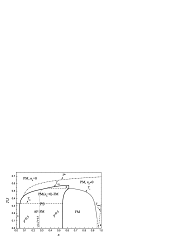
Figure 4: The phase diagram of the model at $\epsilon_{JT}/w_{0}=0.05$, $J/w_{0}=0.01$, $\lambda=10$, $\Omega/w_{0}=0.03$, and $u/w_{0}=0.5$. The numbers denote: 1. homogeneous AF phase; 2. the mixture of two PM states with $n_{b}\neq 0$ and $n_{b}=0$; 3. and 4. homogeneous canted states.

Let us now discuss the transition of the system from the PS to a homogeneous state. The volume fraction of the F phase in the PS state is $p(T)=x/x_{2}(T)$. Depending on the relation between the temperatures $T_{\text{PS}}$, $T_{C}$, $T_{N}$, and $T^{*}$, the system can pass from the PS state to the FM ($p=1$), AF ($p=0$), and PM (with $n_{b}\neq 0$ or $n_{b}=0$) homogeneous states. In all cases, the number of itinerant electrons $n_{b}$ undergoes a sudden change at the transition to the homogeneous state. The temperature dependence of $n_{b}$ is shown in Fig. 5.

Figure 5: The temperature dependence of $n_{b}$ at $x=0.3$, $\epsilon_{JT}/w_{0}=0.05$, $J/w_{0}=0.01$, $\lambda=10$, $\Omega/w_{0}=0.03$, and $u/w_{0}=0.5$.

V Effect of magnetic field

In this section, we consider the effect of magnetic field on the properties of the system. We take into account only the effect of the magnetic field on the local spin. This corresponds to the limit of classical local spin $S\gg 1$. Thus, in the presence of external DC magnetic field $\mathbf{H}$, we should add the term $-\mu_{B}g\sum_{\mathbf{n}}\mathbf{S_{n}}\mathbf{H}$ in Hamiltonian (2), where $\mu_{B}$ is the Bohr magneton and $g$ is the Lande factor. As a result, the magnetic field term modifies only the magnetic Hamiltonian, Eq. (5),

$$H_{\text{m}}=-\sum_{\langle{\bf nm}\rangle}\left[\left\langle c^{{\dagger}}_{{\bf n}}c_{{\bf m}}\right\rangle\left(t\sqrt{\frac{1+\mathbf{e}_{\mathbf{n}}\mathbf{e}_{\mathbf{m}}}{2}}-\bar{t}\right)\right.$$ (41)

$$\left.\phantom{\frac{H_{\text{m}}}{2}}-J^{\prime}S^{2}\mathbf{e_{n}}\mathbf{e_{m}}+\mathbf{e_{n}h}\right],\,\,\,\,\,\,\,\mathbf{h}=\mu_{B}gS\mathbf{H}\,.$$

In the FM state, the one-site magnetic Hamiltonian (25) corresponding to the MF approximation takes the form

$$H_{m0}(\cos\theta) = -A\left(\frac{\epsilon_{JT}}{\bar{w}}\right)\left(w(T)\sqrt{\frac{1+m\cos\theta}{2}}-\bar{w}\right)$$ (42)

$$+Jm\cos\theta-h\cos\theta\,,$$

where the direction of magnetic field is parallel to $z$ axis. The mean value $m=\langle S^{z}_{0}\rangle/S$ is found by solving the system of equations (26) and (27) with Hamiltonian (42). At $T<T_{C}$, the correction to the free energy in the presence of magnetic field $\delta F\sim-h$, whereas in paramagnetic phase $\delta F\sim-h^{2}/T_{C}$.

In the AF or canted states, the result depends on the mutual orientation of $\mathbf{h}$ and the vector $\mathbf{l}=(\langle\mathbf{e}_{0}\rangle-\langle\mathbf{e_{\Delta}}\rangle)/2$. The minimum of the free energy corresponds to the case $\mathbf{h}\bot\mathbf{l}$. Let the vector $\mathbf{l}$ be parallel to $z$ axis and the magnetic field $\mathbf{h}$ be parallel to the $x$ axis. The mean values of the directions of local spins in two sublattices, $\langle\mathbf{e}_{0}\rangle$ and $\langle\mathbf{e_{\Delta}}\rangle$ can be written as $\langle\mathbf{e}_{0}\rangle=\{m,\,0,\,l\}$, $\langle\mathbf{e_{\Delta}}\rangle=\{m,\,0,\,-l\}$, where $m$ is proportional to the magnetization of the system. The one-site magnetic Hamiltonian then has the form

$$H_{m0}(\theta,\phi) = -A\left(\frac{\epsilon_{JT}}{\bar{w}}\right)\left(w(T)\sqrt{\frac{1+\mathbf{e}_{0}\langle\mathbf{e_{\Delta}}\rangle}{2}}-\bar{w}\right)$$ (43)

$$+J\mathbf{e}_{0}\langle\mathbf{e_{\Delta}}\rangle-h\sin\theta\cos\phi\,,$$

where $\mathbf{e}_{0}=\{\sin\theta\cos\phi,\,\sin\theta\sin\phi,\,\cos\theta\}$ and

$$\mathbf{e}_{0}\langle\mathbf{e_{\Delta}}\rangle=-l\cos\theta+m\sin\theta\cos\phi\,.$$

The values of $l$ and $m$ are found from the equations

$$\left\{\begin{array}[]{rcl}l&=&\displaystyle\frac{\int d\mathbf{\Omega}\,\cos\theta\,\text{e}^{-\beta H_{m0}(\theta,\phi)}}{\int d\mathbf{\Omega}\,\text{e}^{-\beta H_{m0}(\theta,\phi)}}\\ \\ m&=&\displaystyle\frac{\int d\mathbf{\Omega}\,\sin\theta\cos\phi\,\text{e}^{-\beta H_{m0}(\theta,\phi)}}{\int d\mathbf{\Omega}\,\text{e}^{-\beta H_{m0}(\theta,\phi)}}\,.\end{array}\right.$$ (44)

Expression for the effective bandwidth $\bar{w}$ (33) now takes the form

$$\bar{w}(H,T)=\frac{w(T)}{\sqrt{2}}\displaystyle\frac{\int d\mathbf{\Omega}\sqrt{1+\mathbf{e}_{0}\langle\mathbf{e_{\Delta}}\rangle}\,\,\text{e}^{-\beta H_{m0}(\theta,\phi)}}{\int d\mathbf{\Omega}\,\text{e}^{-\beta H_{m0}(\theta,\phi)}}\,.$$ (45)

At high magnetic fields $h\sim T_{N}\sim J$, we get from Eq. (44) that $l=0$, and the system passes from the AF or canted state to the FM one. The typical Néel temperature in manganites is $T_{N}\sim 100$ K, and the value of $h=J$ corresponds to the fields of the order of $H\sim 100$ T.

If $h/J\ll 1$, the system (44) can be solved perturbatively. The correction to the free energy of the AF state is $\delta F\sim-h^{2}/T_{N}$ both below and above $T_{N}$, because there is no spontaneous magnetization in the system at $H=0$. The external magnetic field favors the FM state in comparison to the AF and canted states. In particular, it reduces the temperature of transition from the AF to FM state. The magnetic field leads to the increase in the effective hopping integral $\bar{t}$ due to the alignment of local spins and thus to the growth in the number of $b$ electrons and the value of $T^{*}$. At the transition from the PS to PM homogeneous state the magnetic field results in the increase of the transition temperature, and the difference $\Delta T_{\text{PS}}=T_{\text{PS}}(H)-T_{\text{PS}}(0)\sim h$. At the transition from the PS to FM state, $\Delta T_{\text{PS}}$ can be both positive and negative depending on the parameters.

Figure 6: The temperature dependence of $(n_{b}(h)-n_{b}(0))/n_{b}(0)$ at $h/J=0.2$, $x=0.3$, $\epsilon_{JT}/w_{0}=0.05$, $J/w_{0}=0.01$, $\lambda=10$, $\Omega/w_{0}=0.03$, and $u/w_{0}=0.3$.

As was mentioned above, the number of itinerant electrons $n_{b}$ differs significantly below and above $T_{\text{PS}}$. Therefore, the shift of the transition temperature $T_{\text{PS}}$ with the magnetic field gives rise to a significant change in the number of itinerant electrons. The temperature dependence of the ratio $(n_{b}(H)-n_{b}(0))/n_{b}(0)$ near the transition temperature $T_{\text{PS}}(0)$ is shown in Fig. 6. The narrow peak in this ratio is a manifestation of the step in $n_{b}(T)$ shown in Fig. 5. Since the position $T_{\text{PS}}$ of the step in $n_{b}(T)$ depends on the magnetic field, a small change in $H$ causes a significant change in the number of charge carriers at a fixed temperature near $T_{\text{PS}}$. The number of itinerant charge carriers determines the value of metallic conductivity of the system. Thus, the large change of $n_{b}$ in magnetic field can be related to the colossal magnetoresistance effect.

VI Conclusions

We discussed a ”minimal model” dealing with the competition between the localization and metallicity in manganites. The Hamiltonian of the model takes into account the essential physics of strongly correlated electron systems with the Jahn-Teller ions: it is, in fact, the Hubbard model with the strong electron-lattice interaction, the Hund’s rule intraatomic coupling, and AF interatomic exchange between local spins. Such an approach provides a possibility to understand the difference between the number of itinerant charge carriers $n_{b}$ and the doping level prlKRS . It is shown that $n_{b}$ can be significantly lower than the number of the charge carriers implied by the doping level. The models of similar type were discussed in Refs. Rama, ; Rama1, ; Pai, . However, the possibility of the phase separation was not considered in these papers.

Here we demonstrate that in the framework of our model phase separation can exist in a wide range of intermediate doping concentrations disappearing at low and high doping level. These predictions are in agreement with the general features of the experimentally found phase diagrams of manganites dagbook ; Dag ; Nag . The obtained results suggest the existence of the droplet-type of the electronic phase separation that was widely discussed in literature (see, e.g., Ref. dagbook, ). We calculated the relative content of different phases in the phase separated states and found the size of such droplets (ferrons). For the characteristic values of parameters, a droplet includes 10–30 unit cells. These results could, in particular, serve as a key to an adequate description of the transport properties of manganites that could not be done in the framework of the single-band models prbMi ; zhetf04 .

As it was mentioned above, various models related to the strongly correlated electrons exhibit a pronounced tendency toward phase separation. The effective Hamiltonian of our model (2) is, in fact, a generalization of the Falicov-Kimball model fal . The latter model describes a system with the hybridization of an electronic band and a localized level. The Falicov-Kimball model is often used as a toy model in the analysis of heavy-fermion materials and it also leads to the phase separation phenomena PSfal . So, we believe that our approach could be applicable not only to manganites but also to a wider class of strongly correlated electron systems. Note that the analogy between the Falicov-Kimball model and the Hamiltonian of the $s-d$ type with the Jahn-Teller interaction was indicated in Ref. Pai, but in the case without phase separation.

In this paper, we analyzed the phase diagram of the model in the $x-T$ plane. The effect of temperature manifests itself mainly in the change of effective hopping integral $t$ due to the polaron band narrowing and the entropy term in the free energy due to thermal fluctuations of local spins. The polaron band narrowing is described by standard formula (3), see Refs. polaron, ; KH, . The behavior of the local spins was treated using the mean field approximation. We find that at low temperatures the system is in a state with a long-range magnetic order: AF, FM or AF–FM phase separated state. We demonstrate that at high temperatures there can exist two types of the paramagnetic state, a usual one with $n_{b}=0$ and that with $n_{b}\neq 0$. In the intermediate temperature range, the phase diagram includes different kinds of the PS states: AF–FM, FM–PM, and PM with different content of itinerant electrons.

The applied magnetic field leads to the changes in the phase diagram. It evidently favors the FM ordering and, consequently, to the increase of the number of itinerant electrons. The effect of the magnetic field was analyzed accounting for the alignment of the local spins in the applied magnetic field.

It is demonstrated that in our model the metal-insulator transition can take place at some characteristic values of the doping $x$ corresponding to the crossover between different kinds of the phase separation. It can be induced by changing temperature or the magnetic field and is of a percolation type. This transition can be related to the colossal magnetoresistance effect.

Note that in the present treatment we assume that the effective parameters $t$ and $\epsilon_{\text{JT}}$ do not depend on the doping level $x$. To verify the applicability of such approximation, we calculated the phase diagram with $t$ and $\epsilon_{\text{JT}}$ depending linearly on $x$. We found that the phase diagram remains qualitatively the same even if $t$ and $\epsilon_{\text{JT}}$ vary by the factor 2–3 provided the hierarchy of the model parameters ($J\ll\epsilon_{JT}<w_{0}$) remains unchanged.

Note also that we included to our analysis the long-range Coulomb interaction related to the macroscopic charge redistribution in the phase separated state. It allowed us to estimate the size of the inhomogeneities. At the same time, we did not take explicitly into account the corresponding terms in the model Hamiltonian (2). However, if we would like to consider the effect of charge ordering, we have to include at least the nearest-neighbor Coulomb repulsion.

Here we considered only the ”minimal model” describing the effect of the phase separation. Therefore, we did not include into consideration the possibility of the charge ordering to focus the discussion on the interplay between localized and itinerant electrons. It is not impossible to include the charge ordering to the model of such type. The first attempt was made in Ref. Rama1, , but the possibility of phase separation was not considered there. The effect of the charge ordering could change the results for $x$ near 0.5. Therefore, it is reasonable to consider only the range $x<0.5$, if we want to compare our predictions with the actual situation in the doped magnetic oxides.

Appendix A Surface energy

In this section, we calculate the surface energy coming from the size quantization. The expression for the free energy of $b$ and $l$ electrons can be written in terms of the density of states in the form (see Eqs. (19) and (24))

$$F_{\text{el}}=\bar{w}(1-n_{l})^{2}\int\limits_{-1}^{\mu^{\prime}}dE^{\prime}\,E^{\prime}\rho_{0}(E^{\prime})-\epsilon_{JT}n_{l}\,,$$ (46)

where

$$\mu^{\prime}=-\frac{\epsilon_{JT}}{\bar{w}(1-n_{l})}\,.$$

This expression is valid for $x<x_{2}(T)$ and $\mu=-\epsilon_{JT}$. The density of states for the system of itinerant electrons in the volume $V$ is

$$\rho_{0}(E^{\prime})=\frac{1}{V}\sum_{{\bf n}}\,\delta\left(E^{\prime}-\zeta({\bf k_{n}})\right)\,,$$ (47)

where momentum ${\bf k}$ varies over a discrete set of values, depending on boundary conditions and geometry of the system. The function $\zeta({\bf k_{n}})$ is normalized to unity, that is $|\zeta({\bf k_{n}})|\leq 1$. In the thermodynamic limit $V\to\infty$, the sum in Eq. (47) can be replaced by the integral over ${\bf k}$ in the first Brillouin zone multiplied by $V/(2\pi)^{3}$. At finite $V$, we derive an approximate expression for the density of states in the case of cubic lattice, corresponding a small value of $\Delta=Sd/V$, where $S$ is the surface area and $d$ is the lattice constant.

Let the sample has the shape of a parallelepiped $P$ with sides $L_{1}$, $L_{2}$, and $L_{3}$ (in units of the lattice constant $d$). The Dirichlet boundary conditions for the conduction electron wave function $\psi_{\bf m}$ is used, that is, $\psi_{\bf m}=0$ for ${\bf m}\,\nexists\,P$. In this case, the momentum ${\bf k_{n}}$ takes values ${\bf k_{n}}=\pi{\bf n}/(L_{\alpha}+1)$, where $n^{\alpha}=1,\,2\dots\,L_{\alpha}$ ($\alpha=1,\,2,\,3$). For large $L_{\alpha}$, we can use the trapezium rule for the sum over $k^{\alpha}$

$$\sum_{n=1}^{L_{\alpha}}f(k^{\alpha}_{n})=\frac{L_{\alpha}+1}{\pi}\!\!\int\limits_{0}^{\pi}\!\!dk\,f(k)-\frac{1}{2}(f(0)+f(\pi))+O\left(\frac{1}{L_{\alpha}}\right).$$

As a result, for 3D sum over ${\bf n}$ we obtain

$$\sum\limits_{\bf n} f({\bf k_{n}})\simeq\left(V+\frac{S}{2}\right)\!\!\int\!\!\frac{d^{3}k}{\pi^{3}}\,f({\bf k})$$

$$- \frac{V}{2}\left(\int\!\!\frac{d^{2}k}{\pi^{2}L_{1}}\left[f(\{0,k^{2},k^{3}\})+f(\{\pi,k^{2},k^{3}\})\right]\right.$$

$$+ \!\!\!\!\int\!\!\frac{d^{2}k}{\pi^{2}L_{2}}\left[f(\{k^{1},0,k^{3}\})+f(\{k^{1},\pi,k^{3}\})\right]$$

$$+ \left.\!\!\int\!\!\frac{d^{2}k}{\pi^{2}L_{3}}\left[f(\{k^{1},k^{2},0\})+f(\{k^{1},k^{2},\pi\})\right]\right)\,,$$

where 3D and 2D momentum integrations are performed in the range $0\leq k^{\alpha}\leq\pi$, and $S=2(L_{1}L_{2}+L_{1}L_{3}+L_{2}L_{3})$ is the surface area of the parallelepiped in the units of lattice constant.

Using formula (A) with $f({\bf k})=\delta(E^{\prime}-\zeta({\bf k}))$, we can calculate the density of states. Relation (A) can be simplified for the case of cubic symmetry since $\zeta(k^{1},k^{2},k^{3})=\zeta(k^{2},k^{1},k^{3})=\zeta(k^{3},k^{2},k^{1})$. In the absence of external fields, we have $\zeta({\bf k})=\zeta(-{\bf k})$, and the integration in Eq. (A) can be extended to $-\pi\leq k^{\alpha}\leq\pi$. As a result, we obtain for the density of states

$$\rho(E^{\prime})=\left(1+\frac{\Delta}{2}\right)\rho_{0}(E^{\prime})-\frac{\Delta}{4}\int\frac{d^{2}p}{(2\pi)^{2}}\,\left[\delta\left(E^{\prime}-\zeta(\{0,p^{1},p^{2}\})\right)+\delta\left(E^{\prime}-\zeta(\{\pi,p^{1},p^{2}\})\right)\right]\,,$$ (49)

where $\rho_{0}(E^{\prime})$ is the density of states at $V\to\infty$. Note, that the density of states in the form (49) depends only on the ratio $S/V$ and does not depend on the shape of the sample. We believe, that Eq. (49) is applicable for any geometry of the system, provided that the minimum linear dimension $L$ is large compared to the lattice constant (see, for example BB ; Ivan ).

Let us calculate now the surface energy for the spectrum in the tight-binding approximation for the simple cubic lattice, $\zeta({\bf k})=-[\cos(k^{1}d)+\cos(k^{2}d)+\cos(k^{3}d)]/3$. In the limit $V\to\infty$, the formulas for the density of states $\rho_{0}(E^{\prime})$, density of itinerant electrons $n_{0}(\mu)$, and their kinetic energy $\varepsilon_{0}(\mu)$ can be written in the following form

$$\rho_{0}(E^{\prime}) = \int\limits_{0}^{+\infty}\frac{du}{\pi}\,J_{0}^{3}\left(\frac{u}{3}\right)\cos(E^{\prime}u)\,,$$ (50)

$$n_{0}(\mu^{\prime}) = \int\limits_{0}^{+\infty}\frac{du}{\pi}\,J_{0}^{3}\left(\frac{u}{3}\right)\frac{\sin(u)+\sin\left(\mu^{\prime}u\right)}{u}\,,$$ (51)

$$\varepsilon_{0}(\mu^{\prime}) = \int\limits_{0}^{\infty}\frac{du}{\pi}\,J_{0}^{3}\left(\frac{u}{3}\right)\left[\frac{\mu^{\prime}\sin(\mu^{\prime}u)-\sin(u)}{u}\right.$$ (52)

$$\left.+\frac{\cos(\mu^{\prime}u)-\cos(u)}{u^{2}}\right]\,,$$

where $J_{0}$ is the Bessel function. Now, Eq. (49) can be rewritten as

$$\rho(E^{\prime}) = \left(1+\frac{\Delta}{2}\right)\rho_{0}(E^{\prime})$$

$$-\frac{\Delta}{4}\left(\rho^{(2)}_{0}(E^{\prime}+1/3)+\rho^{(2)}_{0}(E^{\prime}-1/3)\right)\,,$$

where

$$\rho^{(2)}_{0}(E^{\prime})=\int\limits_{0}^{+\infty}\frac{du}{\pi}\,J_{0}^{2}\left(\frac{u}{3}\right)\cos(E^{\prime}u)$$ (54)

is the density of states in the 2D case. The number $n_{l}$ and the free energy of electrons (in the case $n_{l}\neq 0$) is given by Eqs. (15) and (46), where instead of $\rho_{0}(E^{\prime})$ we should use the density of states Eq. (A). Note that $n_{l}$ and $F_{\text{el}}$ are functions of $\Delta$. In the considered limit $\Delta\ll 1$, we can use the perturbation technique to calculate the surface energy $\sigma$. Representing the number of $l$ electrons and the free energy $F_{\text{el}}$ in the form $n_{l}=n_{l}^{(0)}+\Delta\,n_{l}^{(1)}+\dots$, $F_{\text{el}}=F_{\text{el}}^{(0)}+\Delta\,\sigma+\dots$, and expanding Eqs. (15), (16), and (46), one obtains

$$n_{l}^{(1)} = -\frac{1}{2}\left(1-n_{l}^{(0)}\right)$$

$$\times\frac{n_{0}(\mu_{0}^{\prime})-\frac{1}{2}\left(n_{0}^{(2)}(\mu_{0}^{\prime}+\frac{1}{3})+n_{0}^{(2)}(\mu_{0}^{\prime}-\frac{1}{3})\right)}{1-n_{0}(\mu_{0}^{\prime})+\mu_{0}^{\prime}\rho_{0}(\mu_{0}^{\prime})}\,,$$

$$\sigma = \bar{w}\left\{(1-n_{l}^{(0)})\left(\mu_{0}^{\prime 2}\rho_{0}(\mu_{0}^{\prime})-2\varepsilon_{0}(\mu_{0}^{\prime})\right)-\frac{\epsilon_{\text{JT}}}{\bar{w}}\right\}n_{l}^{(1)}$$

$$+ \left\{2\varepsilon_{0}(\mu_{0}^{\prime})-\varepsilon^{(2)}_{0}(\mu_{0}^{\prime}+\frac{1}{3})-\varepsilon^{(2)}_{0}(\mu_{0}^{\prime}-\frac{1}{3})\right.$$

$$+ \left.\frac{1}{3}\left[n_{0}^{(2)}(\mu_{0}^{\prime}+\frac{1}{3})-n_{0}^{(2)}(\mu_{0}^{\prime}-\frac{1}{3})\right]\right\}\frac{\bar{w}(1-n_{l}^{(0)})^{2}}{4},$$

where $n_{l}^{(0)}$ is determined by Eq. (15) at $\Delta=0$, $\mu_{0}^{\prime}=-\epsilon_{\text{JT}}/[\bar{w}(1-n_{l}^{(0)})]$, $n_{0}^{(2)}(\mu^{\prime})$ and $\varepsilon^{(2)}_{0}(\mu^{\prime})$ are the number of $b$ electrons and their energy in 2D case at $\Delta=0$,

$$n_{0}^{(2)}(\mu^{\prime}) = \int\limits_{0}^{+\infty}\frac{du}{\pi}\,J_{0}^{2}\left(\frac{u}{3}\right)\frac{\sin\left(\frac{2u}{3}\right)+\sin(\mu^{\prime}u)}{u}\,,$$ (57)

$$\varepsilon_{0}^{(2)}(\mu^{\prime}) = \int\limits_{0}^{\infty}\frac{du}{\pi}\,J_{0}^{2}\left(\frac{u}{3}\right)\left[\frac{\mu^{\prime}\sin(\mu^{\prime}u)-\frac{2}{3}\sin\left(\frac{2u}{3}\right)}{u}\right.$$ (58)

$$\left.+\frac{\cos(\mu^{\prime}u)-\cos\left(\frac{2u}{3}\right)}{u^{2}}\right]\,.$$

At doping concentration $x>x_{2}(T)$ when $n_{l}=0$, we should use the equation $1-x=n_{0}(\mu^{\prime})$ for the chemical potential, where $\rho_{0}(E^{\prime})$ is substituted by $\rho(E^{\prime})$. As a result, we obtain the expression for the surface energy

$$\sigma = \frac{\bar{w}\mu_{0}^{\prime}}{4}\left\{n_{0}^{(2)}(\mu_{0}^{\prime}+\frac{1}{3})+n_{0}^{(2)}(\mu_{0}^{\prime}-\frac{1}{3})-2n_{0}(\mu_{0}^{\prime})\right\}$$ (59)

$$+ \frac{\bar{w}}{2}\left\{\varepsilon_{0}(\mu_{0}^{\prime})-\frac{1}{2}\left[\varepsilon^{(2)}_{0}(\mu_{0}^{\prime}+\frac{1}{3})+\varepsilon^{(2)}_{0}(\mu_{0}^{\prime}-\frac{1}{3})\right]\right.$$

$$+ \left.\frac{1}{6}\left[n_{0}^{(2)}(\mu_{0}^{\prime}+\frac{1}{3})-n_{0}^{(2)}(\mu_{0}^{\prime}-\frac{1}{3})\right]\right\},$$

where $\mu_{0}^{\prime}$ is found from the equation $1-x=n_{0}(\mu_{0}^{\prime})$ at $\Delta=0$. The dependence $\sigma(x)$ is shown in Fig. 7. The function $\sigma(x)$ is discontinuous at $x=x_{2}(T)$. This singularity stems from the kink in the free energy $F_{\text{el}}(x)$ (see Fig. 3).

Figure 7: The surface energy vs doping concentration $x$ at $\epsilon_{\text{JT}}/\bar{w}=0.1$.

In the approximation under discussion, the corresponding corrections to the magnetic contribution to the free energy $F_{m}$ are of the order of $\Delta^{2}$, and therefore we omit them.

References

• (1) E. Dagotto, Science 309, 257 (2005); New J. Phys. 7, 67 (2005).
• (2) E. L. Nagaev, Usp. Fiz. Nauk 165, 529 (1995)[Physics-Uspekhi 38, 497 (1995)].
• (3) A. H. Castro Neto and B. A. Jones Phys. Rev. B62, 14975 (2000); P. Chandra, P. Coleman, J. A. Mydosh, and V. Tripathi, Nature (London) 417, 831 (2002).
• (4) E. Dagotto, Nanoscale Phase Separation and Colossal Magnetoresistance: The Physics of Manganites and Related Compounds (Springer-Verlag, Berlin, 2003).
• (5) P. L. Kuhns, M. J. R. Hoch, W. G. Moulton, A. P. Reyes, J. Wu, and C. Leighton, Phys. Rev. Lett. 91, 127202 (2003).
• (6) G. Blumberg, M. V. Klein, and S.-W. Cheong, Phys. Rev. Lett. 80, 564 (1998); R. Lemanski, J. K. Freericks, and G. Banach, Phys. Rev. Lett. 89, 196403 (2002).
• (7) H. Seo, C. Hotta, and H. Fukuyama, Chem. Rev., 104, 5005 (2004).
• (8) E. L. Nagaev, Pis’ma v ZhETF 6, 484 (1967) [JETP Lett. 6, 18 (1967)].
• (9) T. Kasuya, A. Yanase, and T. Takeda, Solid State Commun. 8, 1543, 1551 (1970).
• (10) A. M. Balagurov, V. Yu. Pomjakushin, D. V. Sheptyakov, V. L. Aksenov, P. Fischer, L. Keller, O. Yu. Gorbenko, A. R. Kaul, and N. A. Babushkina, Phys. Rev. B64, 024420 (2001).
• (11) M. Uehara, S. Mori, C. H. Chen, and S.-W. Cheong, Nature (London) 399, 560 (1999).
• (12) M. Yu. Kagan, K. I. Kugel, and D. I. Khomskii, Zh. Teor. Eksp. Fiz. 120, 470 (2001) [JETP 93415 (2001)].
• (13) S. Mori, C. H. Chen, and S.-W. Cheong, Nature (London) 392, 473 (1998); P. G. Radaelli, D. E. Cox, L. Capogna, S.-W. Cheong, and M. Marezio, Phys. Rev. B59, 14440 (1999); B. Raveau, M. Hervieu, A. Maignan, and C. Martin, J. Mater. Chem. 11, 29 (2001).
• (14) D. I. Khomskii and K. I. Kugel, Phys. Rev. B67, 134401 (2003).
• (15) M. Yu. Kagan and K. I. Kugel, Usp. Fiz. Nauk. 171, 577 (2001) [Physics - Uspekhi 44, 553 (2001)].
• (16) V. J. Emery, S. A. Kivelson, and H. Q. Lin, Phys. Rev. Lett. 64, 475 (1990).
• (17) P. B. Visscher, Phys. Rev. B10, 943 (1974).
• (18) J. K. Freericks, Ch. Gruber, and N. Macris, Phys. Rev. B60, 1617 (1999); J. K. Freericks, E. H. Lieb, and D. Ueltschi, Phys. Rev. Lett. 88, 106401 (2002); M. M. Maśka and K. Czajka, phys. stat. sol. (b) 242, 479 (2005).
• (19) J. H. Zhao, H. P. Kunkel, X. Z. Zhou, and G. Williams, Phys. Rev. B66, 184428 (2002).
• (20) A. L. Rakhmanov, K. I. Kugel, Ya. M. Blanter, and M. Yu. Kagan, Phys. Rev. B63, 174424 (2001).
• (21) K. I. Kugel, A. L. Rakhmanov, A. O. Sboychakov, M. Yu. Kagan, I. V. Brodsky, and A. V. Klaptsov, Zh. Eksp. Teor. Fiz. 125, 648 (2004) [JETP 98, 572 (2004)].
• (22) K. I. Kugel, A. L. Rakhmanov, and A. O. Sboychakov, Phys. Rev. Lett. 95, 267210 (2005).
• (23) A. J. Millis, P. B. Littlewood, and B. I. Shraiman, Phys. Rev. Lett. 74, 5144 (1995).
• (24) J. Bala, P. Horsch, and F. Mack, Phys. Rev. B69, 094415 (2004).
• (25) M. Gulacsi, A. Bussmann-Holder, and A. R. Bishop, Phys. Rev. B71, 214415 (2005).
• (26) T. V. Ramakrishnan, H. R. Krishnamurthy, S. R. Hassan, and G. V. Pai, Phys. Rev. Lett. 92, 157203 (2004).
• (27) O. Cépas, H. R. Krishnamurthy, and T. V. Ramakrishnan, Phys. Rev. Lett. 94, 247207 (2005).
• (28) J. B. Goodenough, Magnetism and the Chemical Bond (Interscience, New York, 1963).
• (29) C. Zener, Phys. Rev. 82, 403 (1951).
• (30) G. V. Pai, S. R. Hassan, H. R. Krishnamurthy, and T. V. Ramakrishnan, Europhys. Lett. 64, 696 (2003).
• (31) P. G. de Gennes, Phys. Rev. 118, 141 (1960).
• (32) A. S. Alexandrov and N. F. Mott, Polarons and Bipolarons (World Scientific, Singapore, 1995).
• (33) K. I. Kugel and D. I. Khomskii, Zh. Eksp. Teor. Fiz. 79, 987 (1980) [Sov. Phys. JETP 52, 501 (1980)].
• (34) J. S. Smart, Effective Fields Theories of Magnetism, (Saunders, London, 1966).
• (35) L. D. Landau and E. M. Lifshitz, Statistical Physics (Butterworth-Heinemann, Oxford, 1980), Part 1.
• (36) J. Lorenzana, C. Castellani, and C. di Castro, Europh. Lett. 57, 704 (2002).
• (37) E. Dagotto, T. Hotta, and A. Moreo, Phys. Reports 344, 1 (2001).
• (38) E. L. Nagaev, Phys. Reports 346, 387 (2001).
• (39) L. M. Falicov and J. C. Kimball, Phys. Rev. Lett. 22, 997 (1969).
• (40) R. Balian and C. Bloch, Ann. Phys. (N.Y.) 60, 401 (1970).
• (41) I. González, J. Castro, and D. Baldomir, Phys. Lett. A 298, 185 (2002).