Quantum Logic Processor: A Mach Zehnder Interferometer based Approach

Abstract

Quantum Logic Processors can be implemented with Mach Zehnder Interferometer(MZI) configurations for the Quantum logic operations and gates. In this paper, its implementation for both optical and electronic system has been presented. The correspondence between Jones matrices for photon polarizations and Pauli spin matrices for electrons gives a representation of all the unitary matrices for the quantum gate operations. A novel quantum computation system based on a Electronic Mach Zehnder Interferometer(MZI) has also been proposed. It uses the electron spin as the primary qubit. Rashba effect is used to create Unitary transforms on spin qubits. A mesoscopic Stern Gerlach apparatus can be used for both spin injection and detection. An intertwined nanowire design is used for the MZI. The system can implement all single and double qubit gates. It can easily be coupled to form an array. Thus the Quantum Logic Processor (QLP) can be built using the system as its prototype.

1 INTRODUCTION

According to the ITRS (International Technology Roadmap for Semiconductors) Roadmap [1], the channel length of CMOS should diminish to 22nm by the year 2015 to maintain the ever increasing computing demands. As dimensions shrink further, the atomistic limitations will come into light and Boolean Logic will start to fail. To continue further scaling and improve computing power, Quantum Logic will become inevitable. Nevertheless the experimental realization of quantum logic has not been so impressive.

Preskill [2] has estimated that to have a reliability of 10^-6 atleast 10⁶ qubits must be present in the quantum logic system. Such a large number of qubits is easily possible in a solid state system only. Thus, tremendous improvements have been made in the field of solid state quantum computation in the last 7 years e.g. Nuclear Magnetic Resonance (NMR) [3],electrons floating on liquid helium [4], quantum dots [5], terahertz cavity quantum electrodynamics [6], Cooper-pair box [7], superconducting quantum interference loop [8], ion trap quantum computer [9] spin in silicon [10] etc. Nevertheless the experimental realization of solid state systems are still nowhere near Preskill’s vision. In this project we devise a scheme of implementation of quantum logic in an electronic Mach Zehnder Interferometer.

This paper has been arranged as follows-a fleeting glance of quantum computing and MZI has be given in the beginning. This will be followed by the implementation of various quantum logic gates using the optical MZI. Then we show the transformation of the scheme used in optical MZI to electronic MZI. Finally, the scheme of implementation of quantum logic using electronic MZI will be detailed.

2 QUANTUM COMPUTING: AN OVERVIEW

Quantum computation and information is the study of the information processing tasks that can be accomplished using quantum mechanical systems. But it may be argued that today’s computers are using nano-sized components where quantum effects play a big role. So are these computers built on ’quantum mechanical systems’ quantum computers? The answer is NO. It is because the logic on which the computer operates is classical rather than quantum mechanical.
Just as the classical computation is built upon bits, quantum computation also has an analogous concept called qubits. The main difference between a bit and a qubit is that while a bit can be either 0 or 1, a qubit can be in a superposition of states $\left|0\right\rangle$ and $\left|1\right\rangle$ (where $\left|~{}\right\rangle$ is the Dirac notation). It is possible to form a linear combination of states called superposition:

$$\left|\Psi\right\rangle=\alpha\left|0\right\rangle+\beta\left|1\right\rangle$$ (1)

$\alpha$ and $\beta$ are complex numbers such that $\left|\alpha\right|^{2}+\left|\beta\right|^{2}=1$. A qubit can be geometrically represented by a Bloch sphere as seen in Fig. 1.

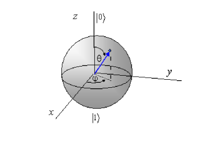
Figure 1: The Bloch Sphere

Analogous to classical computation, the operations on qubits are carried out using quantum logic gates.

3 MZI: AN OVERVIEW

The ubiquitous Mach Zehnder Interferometer was discovered almost a century ago. The simple structure is as shown in Fig 2 [11].

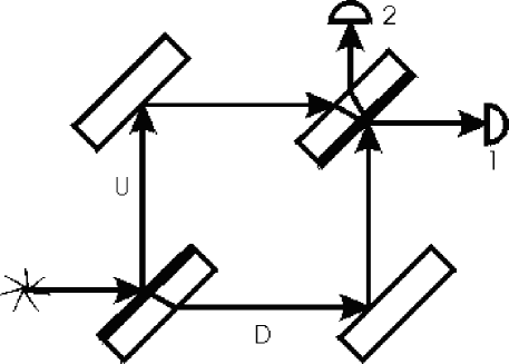
Figure 2: The optical Mach Zehnder Interferometer

ELEMENT	SYMBOLS
Light Source
50-50 Beam Splitter
Totally reflecting mirror
Detector

Different elements can be put in either of the paths of Mach Zehnder Interferometer for manipulating the output states. Fig 3. shows a phase shifter in one of the paths.

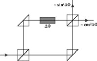
Figure 3: MZI with Phase Shifter

The simple structure has led to numerous uses of the optical MZI since its inception.[12, 13, 14, 15, 16, 17, 18]. It is this flexibility that makes it ideal for quantum computation also.

4 QUANTUM LOGIC IN OPTICAL MZI

The implementation of quantum logic based on optical MZI harnesses photon polarization as qubit. The different polarizations are represented vectorially using Jones vectors[19].The different Jones vectors are tabulated in Table 1.

POLARIZATION	JONES VECTOR
Linear horizontal	$\left[\begin{array}[]{c}1\\ 0\end{array}\right]$
Linear vertical	$\left[\begin{array}[]{c}0\\ 1\end{array}\right]$
Linear at $+45^{o}$	$\frac{1}{\sqrt{2}}\left[\begin{array}[]{c}1\\ 1\end{array}\right]$
Linear at $-45^{o}$	$\frac{1}{\sqrt{2}}\left[\begin{array}[]{c}1\\ -1\end{array}\right]$
Circular, right-handed	$\frac{1}{\sqrt{2}}\left[\begin{array}[]{c}1\\ -\iota\end{array}\right]$
Circular, left-handed	$\frac{1}{\sqrt{2}}\left[\begin{array}[]{c}1\\ \iota\end{array}\right]$

Table 1: Jones Vectors

The elements that are used for manipulating the polarization stated are represented mathematically using Jones Matrices. The Jones Matrices for various optical elements are tabulated in Table 2.

POLARIZATION	JONES MATRIX
Linear horizontal polarizer	$\left(\begin{array}[]{cc}1&0\\ 0&0\end{array}\right)$
Linear vertical polarizer	$\left(\begin{array}[]{cc}0&0\\ 0&1\end{array}\right)$
Linear polarizer at $+45^{o}$	$\frac{1}{2}\left(\begin{array}[]{cc}1&1\\ 1&1\end{array}\right)$
linear polarizer at $-45^{o}$	$\frac{1}{2}\left(\begin{array}[]{cc}1&-1\\ -1&1\end{array}\right)$
Quarter-wave plate,fast axis vertical	$\exp{i\pi/4}\left(\begin{array}[]{cc}1&0\\ 0&-i\end{array}\right)$
Quarter-wave plate, fast axis horizontal	$\exp{i\pi/4}\left(\begin{array}[]{cc}1&0\\ 0&i\end{array}\right)$
Circular polarizer, right-handed	$\frac{1}{2}\left(\begin{array}[]{cc}1&i\\ -i&1\end{array}\right)$
Circular polarizer,left-handed	$\frac{1}{2}\left(\begin{array}[]{cc}1&-i\\ i&1\end{array}\right)$
Beam Splitter	$\frac{1}{\sqrt{2}}\left(\begin{array}[]{cc}1&-1\\ 1&1\end{array}\right)$

Table 2: Jones Matrices

The implementation of various quantum logic gates using optical MZI is tabulated in Table. 3.

Quantum Logic Gate	Unitary Matrix	Relation for MZI	Elements
		implementation
Beam Splitter(B($\theta$))	$\left[\begin{array}[]{cc}cos\theta&-sin\theta\\ sin\theta&cos\theta\end{array}\right]$
50-50 Beam Splitter(B)	$\frac{1}{\sqrt{2}}\left[\begin{array}[]{cc}1&-1\\ 1&1\end{array}\right]$
Hadamard(H)	$\frac{1}{\sqrt{2}}\left[\begin{array}[]{cc}1&1\\ 1&-1\end{array}\right]$	H=BZ	50-50 Beam splitter
Phase flip gate (Z)	$\left[\begin{array}[]{cc}1&0\\ 0&-1\end{array}\right]$	Z=HB	$\pi$ Phase shifter
Bit Flip gate (X)	$\left[\begin{array}[]{cc}0&1\\ 1&0\end{array}\right]$	X=BH	Beam Splitter,
			Hadamard
T gate	$\left[\begin{array}[]{cc}1&0\\ 0&\exp(i\pi/4)\end{array}\right]$		$\pi$/4 phase shifter
S gate	$\left[\begin{array}[]{cc}1&0\\ 0&i\end{array}\right]$		Quarter wave plate
Pauli Y gate	$\left[\begin{array}[]{cc}0&-i\\ i&0\end{array}\right]$
CNOT gate	$\left[\begin{array}[]{cccc}1&0&0&0\\ 0&1&0&0\\ 0&0&0&1\\ 0&0&1&0\end{array}\right]$	(I$\otimes$H)$\times$K$\times$(I$\otimes$H)	$\begin{array}[]{c}\textnormal{Kerr Media(K)}\\ \textnormal{Hadamard(H)}\\ \textnormal{Identity(I)}\end{array}$

Table 3: Quantum Logic Gates

5 ANALOGY BETWEEN ELECTRONS AND PHOTONS

The analogy and similarity between electrons and photons has been noted in Table 4.

PHOTONS	ELECTRONS
Electric Field(E)	Wavefunction($\Psi$)
Polarization	Spin
Poynting Vector(P)	Current Density(J)
$\approx$ Re [E${}^{*}\times$H]	$\approx$ Re[i$\Psi^{*}\times\nabla\Psi$]
$\approx$ Re [-iE${}^{*}\times$$\nabla\times$E]
exp(-i$\omega$t)	exp(-iEt/$\hbar$)
$\omega$-Frequency	E-Energy
$\nabla^{2}$E = $\omega^{2}\mu\epsilon$E	$\nabla^{2}\Psi$ = -(2m/$\hbar^{2}$[E-U]$\Psi$
k2 = $\omega^{2}\mu\epsilon$	k2 = -(2m/$\hbar^{2}$[E-U]

Table 4: Comparison between Electrons and Photons

The similarity of photon polarization and electron spin on which this whole concept of a spin MZI is based must be illustrated further. The comparison between electron spin and photon polarization is shown in Table 5.

PHOTON POLARIZATION	ELECTRON SPIN
Spinor	Spinor
Jones vector	Spin polarization vector
Spin $\pm$1	Spin $\pm$1/2
Jones matrices	Pauli matrices

Table 5: Comparison between Electron Spin and Photon polarization

The realization of various gates and the relation between Jones and Pauli matrices has been shown in the Table 6.

Optical Element	Jones Matrix	Pauli Matrix	Quantum Logic Gate
Linear horizontal polarizer	$\left(\begin{array}[]{cc}1&0\\ 0&0\end{array}\right)$	$I+\sigma_{3}$
Linear vertical polarizer	$\left(\begin{array}[]{cc}0&0\\ 0&1\end{array}\right)$	$I-\sigma_{3}$
Linear polarizer at $+45^{o}$	$\frac{1}{2}\left(\begin{array}[]{cc}1&1\\ 1&1\end{array}\right)$	$\frac{1}{2}[I+\sigma_{1}]$
linear polarizer at $-45^{o}$	$\frac{1}{2}\left(\begin{array}[]{cc}1&-1\\ -1&1\end{array}\right)$	$\frac{1}{2}[I-\sigma_{1}]$
Quarter-wave plate,
fast axis vertical	$\exp{i\pi/4}\left(\begin{array}[]{cc}1&0\\ 0&-i\end{array}\right)$
Quarter-wave plate,
fast axis horizontal	$\exp{i\pi/4}\left(\begin{array}[]{cc}1&0\\ 0&i\end{array}\right)$	Phase Gate
Circular polarizer,
right-handed	$\frac{1}{2}\left(\begin{array}[]{cc}1&i\\ -i&1\end{array}\right)$	$\frac{1}{2}[I-\sigma_{2}]$
Circular polarizer,
left-handed	$\frac{1}{2}\left(\begin{array}[]{cc}1&-i\\ i&1\end{array}\right)$	$\frac{1}{2}[I+\sigma_{2}]$
Beam Splitter	$\frac{1}{\sqrt{2}}\left(\begin{array}[]{cc}1&1\\ 1&-1\end{array}\right)$	$\frac{1}{\sqrt{2}}[\sigma_{1}+\sigma_{3}]$	Hadamard Gate
		$\sigma_{1}$	X Gate
		$\sigma_{3}$	Z Gate

Table 6: Jones and Pauli matrices,a comparison

In Table 6. $\sigma_{i}$ where i=1,2,3) are Pauli Matrices.
The four Pauli Matrices are:

$$I=\sigma_{0}=\left(\begin{array}[]{cc}1&0\\ 0&1\end{array}\right)$$

$$\sigma_{1}=\left(\begin{array}[]{cc}0&1\\ 1&0\end{array}\right)$$

$$\sigma_{2}=\left(\begin{array}[]{cc}0&-i\\ i&0\end{array}\right)$$

$$\sigma_{3}=\left(\begin{array}[]{cc}1&0\\ 0&-1\end{array}\right)$$

Interestingly, $\sigma_{1}$ is NOT (X) gate and $\sigma_{3}$ is Z gate.

6 QUANTUM COMPUTATION WITH ELECTRONIC MZI

Recently, a great interest has been generated in various electronic analogues of optical instruments viz. -the electronic double slit interferometer [20, 21, 22, 23, 24, 25]; spin dependent Fabry Perot Interferometer [26, 27]; electro-optic modulator [28] etc. This is mainly due to exhibition of quantum phase coherence in electronic interference experiments by Aharonov-Bohm oscillations, persistent currents (PC), weak localization, universal conductance fluctuation etc.

This interest has also been extended to MZI. The ubiquitous optical MZI was rediscovered when simulation of quantum logic with optical MZI was presented [29]. An electronic analogue of the MZI was fabricated recently [30] using quantum Hall edge states. In this paper we will extend this interest in MZI with our proposal of an electronic MZI to implement spin based quantum logic gates.

The different elements that can be used for the implementation of quantum logic using a spin MZI is tabulated in Table 7.

Optical Element	Electronic element	Unitary matrix
Polariser/Analyser	Ferromagnetic material which produces spin sub band splitting. The spin which is to be selectively transmitted should have $\vec{P_{0}}$ parallel to $\vec{M}$	Depends on the angle of polarization. However mostly it is like a linear horizontal polarizer $\left[\begin{array}[]{cc}1&0\\ 0&0\end{array}\right]$
Phase Shifter	• Rashba spin orbit interaction • Aharonov Bohm phase • Ferromagnetic material where $\vec{P_{0}}$ is perpendicular to $\vec{M}$	The general matrix of a phase shifter which shifts the phase by $\theta$ is given by $\left[\begin{array}[]{cc}\exp(-i\theta/2)&0\\ 0&1\end{array}\right]$ (up to an unimportant global phase factor).
Polarizing Beam Splitter (PBS)	An arrangement with two beam splitters and a phase shifter.[35]	$\left|\sigma;k\right\rangle\longrightarrow cos\theta\left|\sigma;k\right\rangle+isin\theta\left|\sigma;1-k\right\rangle$ For a beam splitter where $\sigma$ gives the spin degree of freedom and k gives the orbital degree of freedom.
Wave guides	Electrons in 2-DEG
Beam Splitter	• Point contacts • Simple differentiating lines

Table 7: Elements required for implementation of spin MZI

7 DEVICE CONFIGURATION

Electron spin has been used as the primary qubit in our proposed device. All single qubit gates can be realized on the spin qubit using Rashba interaction. However, using the spatial degree of freedom in a electronic Mach Zehnder Interferometer (MZI), the two qubit gates have also been realized. The MZI has been assumed to be free of spin scattering. To ensure this the MZI is expected to be formed by two intertwined ballistic nanowires.

7.1 Design Challenges

There were quite a many challenges in the design of this system. The challenges are discussed one by one.
Magnetic field is normally required for the manipulation of electron spin. Almost all the spin manipulation based quantum computation systems propose to use external magnetic field. Nonetheless, having a different magnetic field in each of the units of the quantum computation system is lithographically very challenging. However,a localized magnetic field in a particular region can be created with the modern technology. Thus the system should be designed so that it should be more or less free of the dependence on the magnetic field. An external magnetic field at a few specified places may be used.
Spin-polarized electrons have been traditionally created in semiconductors simply by illuminating the material with circularly polarized light. Nonetheless, a purely electrical method for injecting spin-polarized electrons into semiconductors is needed to guarantee the success of quantum computing system. In literature, two different concepts have been employed to solve the problem. The first approach involves injecting spins from a dilute magnetic semiconductor(DMS) that acts as an efficient spin aligner when an external magnetic field is applied. This concept works well at low temperatures - almost all the electrically injected electrons have their spins pointing in the same direction. However, it is extremely difficult to implement at room temperature because most of the known magnetic semiconductors lose their spin-aligning characteristics just above liquid-helium temperatures (i.e. above 4 K). The second approach involves injecting spin-polarized electrons from a ferromagnetic material [28], where almost all of the conducting electrons are intrinsically aligned. However, this approach also faces problems. Randomly oriented spins - known as magnetically dead layers - in the ferromagnetic material close to the semiconductor interface are a barrier to effective spin injection Hence, a different spin injection and detection scheme must be proposed to ensure the robustness of the quantum computing system.
CNOT gate is an essential gate for the flexibility of a quantum computation system. Hence the scheme must be able to implement double qubit gates like CNOT.

The strategies adopted for overcoming all the aforementioned challenges are discussed in the following section. A localized magnetic field was created with the aid of Rashba effect using a localized electric field created by a gate. The spin injection and detection problem was solved with the aid of a recently proposed Stern Gerlach apparatus. CNOT gate was also implemented using spin as the target qubit and spatial degree of freedom as the control qubit.

7.2 Rashba Effect in ballistic MZI

Even in the absence of a magnetic field, the spin degeneracy may be lifted due to the coupling of the electron spin and its orbital motion. This mechanism is popularly referred to as the Rashba effect [34]. The spin orbit (Rashba) Hamiltonian is given by

$$H_{R}=\frac{\alpha}{\hbar}\vec{y}\cdot\left[\vec{\sigma}\times\vec{p}\right]$$ (2)

Here y axis has been chosen to be perpendicular to the plane of motion of the electron(the direction of the electric field), $\alpha$ is the spin-orbit coupling coefficient, $\vec{\sigma}$ represents the Pauli spin matrices, $\vec{p}$ is the momentum operator. Typical values of $\alpha$ range from $9\times 10^{-12}$ eV m at electron density of $n=7\times 10^{11}cm^{-2}$ to $6\times 10^{-12}eVm$ at electron density of $n=2\times 10^{12}cm^{-2}$. Due to Rashba interaction, the Fermi sphere splits into two(see Fig 4). Thus a spin dependent band splitting is achieved.

Figure 4: Splitting of the Fermi Sphere

In the limit of $\alpha=0$, the eigen energies are given by

$$E^{0}_{n}=E_{n}+\frac{\hbar^{2}k_{y}^{2}}{2m^{*}}$$ (3)

If we treat the spin orbit interaction using the perturbation model( This model is quite correct as the spin orbit effect is quite weak), the eigenvalues can be written as:

$$E^{\pm}(k_{y}) = E^{0}_{n}\pm\alpha k_{y}$$ (4)

$$E^{\pm}(k_{y}) = E_{n}+\frac{\hbar^{2}k_{y}^{2}}{2m^{*}}\pm\alpha k_{y}$$ (5)

Here n is the subband index, $m^{*}$ is the effective mass. The above equation allows more than one values of $k_{y}$ to have the same energy. Let these values be $k_{y1}$ and $k_{y2}$. Hence,

$$E^{+}(k_{y1})-E^{-}(k_{y2}) = \frac{\hbar^{2}}{2m^{*}}(k_{y1}^{2}-k_{y2}^{2})+\alpha(k_{y1}+k_{y2})$$ (6)

$$= 0$$ (7)

$$k_{y1}-k_{y2} = \frac{2m^{*}\alpha}{\hbar^{2}}=\Delta k_{y}$$ (8)

$$\phi_{R} = \Delta k_{y}L$$ (9)

$$\phi_{R} = \frac{2m^{*}\alpha L}{\hbar^{2}}$$ (10)

Here $\phi_{R}$ represents the phase shift in the Rashba region.L is the length of the Rashba region. The unitary transform associated with this phase shift is

$$U_{R}=exp[\iota\phi_{R}\sigma_{z}]$$ (11)

Thus the effect of the Rashba interaction is to rotate the spin direction by $\phi_{R}$ in the spin space. A point to note here is that in the above derivation, the intersubband coupling was neglected. This approximation is valid if the following condition holds [28]:

$$w\ll\frac{\hbar^{2}}{\alpha m^{*}}$$ (12)

Here w is the width of the ballistic nanowire.

7.3 Mesoscopic Stern Gerlach Apparatus

As mentioned earlier, traditionally, ferromagnetic contacts have been used for spin injection and detection. However it is well known that the same can be done with a Stern Gerlach apparatus in macroscopic domain. Extending this concept, spin injection and detection through a mesoscopic Stern Gerlach Apparatus [35] was proposed for the quantum computing system.

The aforementioned Stern Gerlach Apparatus uses a MZI like structure to produce a Polarizing Beam Splitter(PBS). It is a two input, two output structure and hence is easily compatible with our MZI design. It has Rashba interaction selectively on one of the arms. Also there is flux $\Phi$ threading the apparatus. The outputs can be tuned to have only spin ups and spin downs along different paths. Let us define the two modes to be k=0,1. Let the Rashba interaction be present in only the ‘1’ mode. Hence the transformation can be written as:

$$\left|\uparrow,k\right\rangle \rightarrow e^{\iota k\phi_{R}}\left|\uparrow,k\right\rangle$$ (13)

$$\left|\downarrow,k\right\rangle \rightarrow e^{-\iota k\phi_{R}}\left|\downarrow,k\right\rangle$$ (14)

The magnetic flux $\Phi$ threading the interferometer generates a Aharonov Bohm(AB) phase. This induces a phase difference in the electronic wavefunctions in the two arms. This phase difference can be assumed in the ‘1’ mode without any loss of generality. Thus,

$$\left|\sigma,0\right\rangle \rightarrow \left|\sigma,0\right\rangle$$ (15)

$$\left|\sigma,1\right\rangle \rightarrow e^{\iota\Phi_{AB}}\left|\sigma,1\right\rangle$$ (16)

$$\Phi_{AB} = \Phi/\Phi_{0}$$ (17)

$$\Phi_{0} = \frac{hc}{e}$$ (18)

The net transformation induced by the two mechanisms are as follows (assuming the beam splitter to be 50-50):

$$\left|\uparrow;0\right\rangle \rightarrow t_{0}^{\uparrow}\left|\uparrow;0\right\rangle+t_{1}^{\uparrow}\left|\uparrow;1\right\rangle$$ (19)

$$\left|\downarrow;0\right\rangle \rightarrow t_{0}^{\downarrow}\left|\uparrow;0\right\rangle+t_{1}^{\downarrow}\left|\uparrow;1\right\rangle$$ (20)

$$t_{0}^{\uparrow,\downarrow} = -e^{\iota(\Phi_{AB}\pm\Phi_{R})/2}\iota sin\left(\frac{\Phi_{AB}\pm\Phi_{R}}{2}\right)$$ (21)

$$t_{1}^{\uparrow,\downarrow} = e^{\iota(\Phi_{AB}\pm\Phi_{R})/2}\iota cos\left(\frac{\Phi_{AB}\pm\Phi_{R}}{2}\right)$$ (22)

Choosing $\Phi_{AB}=\Phi_{R}=\pi/2$ ,we get,

$$\left|\uparrow,0\right\rangle \rightarrow \left|\uparrow,0\right\rangle$$ (23)

$$\left|\downarrow,1\right\rangle \rightarrow \iota\left|\downarrow,1\right\rangle$$ (24)

Hence spin injection can be done as required by choosing an appropriate $\Phi_{AB}$ and $\Phi_{R}$. The spin injection can be as high as 100% as both the spin injector and our device can be of the same material. There is no impedance mismatch at the interface.

Single spin detection is a big problem in spintronics. The success of spin systems depends on efficient spin injection and detection. However efficient methods for detection of electron spin directly in solids are still eluding. Nevertheless single charge detection is possible. Hence some proposals for single spin detection in nano devices are based on the swap operation of a spin state to a charge state [10]. Proposals have also been made for spin detection using Scanning Tunneling Microscopy(STM) [36] and Magnetic Resonant Force Microscopy(MRFM) [37, 38].

Single Electron Transistor(SET) can used to detect single electron charge. Thus in our system too, efficient single spin detection can be done by performing the swap operation of a spin state to a charge state. The MSGA performs the swap function efficiently. Hence for spin readout in our system, an MSGA is coupled to the output of the electronic MZI. The output of the MSGA is fed to SET. Again the MSGA can be fabricated in the same material as MZI. Hence the spin detection efficiency would be high.

7.4 Quantum Logic Gates

The realization of different quantum logic gates will be discussed in this section. The quantum logic gates can be implemented in an electronic MZI system.A schematic MZI system with the spatial(modal) and spin qubit has been shown in Fig 5.

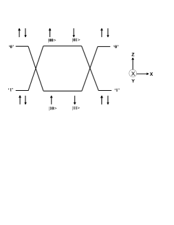
Figure 5: A schematic electronic MZI with the different qubits depicted

The electron spin is the primary qubit in the proposed system. Hence all the single qubit gates have been designed for the spin qubit. It was mentioned in section 7.2 on Rashba effect, that it rotates electron spin in the spin space. Now it is well known that all single qubit gates are nothing but rotations on the Bloch sphere. An electron spin can easily be visualized on the Bloch sphere with the $\uparrow$ and $\downarrow$ on opposite poles. All superposition states can also be represented by points on the Bloch sphere. Thus rotations in spin space correspond to rotations on Bloch sphere (Fig 1). It has already been shown that all rotations can be achieved by varying the spin orbit coupling coefficient $\alpha$. $\alpha$ in turn can be tuned by a gate voltage in a ballistic MZI ( Fig 6).

Figure 6: A schematic ballistic MZI with gates for application of voltage. The Rashba interaction can be controlled by tuning the gate voltages

For an analytical calculation, the device size can be fixed at 50 nm by 30 nm (50 nm is the distance between two consecutive beam splitters, 30 nm is the distance between the centers of the two parallel paths.) The width of the channel is assumed to be 5nm, the length of Rashba interaction is 20nm. In InGaAs/InAlAs system, a similar structure has been fabricated [39]. The effective mass($m^{*}$) is 0.05 $m_{0}$($m_{0}$ is the rest mass of a free electron) in that system. Also the confinement voltage was 0.53 V . In this system the various $\alpha$ values required for various gates are shown in Table 8.

Quantum Logic Gate	Unitary Matrix	$\alpha(\times 10^{-11}eVm)$
50-50 Beam Splitter(B)	$\frac{1}{\sqrt{2}}\left[\begin{array}[]{cc}1&-1\\ 1&1\end{array}\right]$	1.198
Hadamard Gate(H)	$\frac{1}{\sqrt{2}}\left[\begin{array}[]{cc}1&1\\ 1&-1\end{array}\right]$	1.198
Not Gate(X)	$\left[\begin{array}[]{cc}0&1\\ 1&0\end{array}\right]$	2.397
Phase flip gate (Z)	$\left[\begin{array}[]{cc}1&0\\ 0&-1\end{array}\right]$	4.795
T gate	$\left[\begin{array}[]{cc}1&0\\ 0&\exp(i\pi/4)\end{array}\right]$	0.300
S gate	$\left[\begin{array}[]{cc}1&0\\ 0&i\end{array}\right]$	0.599

Table 8: The spin orbit coupling coefficient $\alpha$ required for some standard single qubit quantum logic gates

The values are close to the values obtained in experiments  [39, 40]. Hence the single qubit gates can be easily obtained by the rotation of the spin.

Double qubit gates are an imperative feature of any quantum computing system. To achieve double qubit gates, entanglement has to be obtained. The electrons are constrained to move in either of the two modes, ‘0’ or ‘1’. Hence the spatial location of the electron(the modes) can also used as a qubit. The beam splitter acts on the spatial qubit and can be represented by the U(2) matrix,

$$\left|k;\sigma\right\rangle\rightarrow\cos\theta\left|k;\sigma\right\rangle+\iota\sin\theta\left|1-k;\sigma\right\rangle$$ (25)

Hence the superposition states for the spatial qubit can also be obtained. As shown in Fig 5, the two qubit representations can be depicted with the spatial qubit as the 1st qubit and spin as the next qubit. The first qubit can easily act as the control qubit. If the Rashba field is turned on in the ‘1’ mode only, spin manipulation will occur in that mode only. For example, in the CNOT, gate, the Rashba field is turned on in mode ‘1’ only with $\alpha$ as shown in Table 8 for NOT gate. Thus there is preferential flipping of the spin qubit in the ‘1’ mode only. This is simply the CNOT gate. Similarly controlled Z gate etc can also be obtained. The Bell states can easily be obtained in this system. This will require a Hadamard on the spatial qubit and then a CNOT gate with the spatial qubit as the control qubit.

8 Conclusions

In this paper, Mach Zehnder based quantum computing systems have been presented. All single qubit and double qubit quantum logic gates are feasible in this system. The system can be implemented in a ballistic nanowire MZI system. The specifications suggest that it can be made within the current state-of-the-art technological facilities available.

The device size should be smaller than the phase coherence and spin coherence length. These have been typically reported to be 20 microns [41] and 100 microns [42] respectively. Hence an array of about 1000 MZI units can be placed in an array to perform any complex operation. This could lead to the ultimate Quantum Logic Processor (QLP). The problems of coupling that exist in a static electron spin quantum computation system have been eliminated in our proposed mobile spin qubit representation. Hence it is better suited for implementation of the QLP.

9 Acknowledgements

Angik Sarkar and Ajay Patwardhan acknowledge the help of the NIUS Programme, HBCSE, Mumbai,India.

References

- [1] Avalible at http://public.itrs.net/
- [2] Preskill, J. Reliable quantum computers. Proc. R. Soc. Lond. A 454, 385–410 (1998).
- [3] Isaac L. Chuang, Neil Gershenfeld and Mark Kubinec, Phys. Rev. Lett., 80, 3408 (1998).
- [4] P.M. Platzman and M.I. Dykman, Science, 284, 1967 (1999).
- [5] D. Loss and D. P. DiVincenzo, Phys. Rev. A, 57, 120 (1998).
- [6] M. S. Sherwin, A. Imamoglu, and T. Montroy, Phys. Rev. A, 60, 3508 (1999).
- [7] Y. Nakamura et al., Nature, 398, 786 (1999).
- [8] Ioffe et al., Nature, 398, 679 (1999).
- [9] C. Monroe, Nature, 416, 238 (2002); D. Kielpinski, C. Monroe and D.J. Wineland, Nature, 417, 6890), 709 (2002).
- [10] B. E. Kane, ”A silicon-based nuclear spin quantum computer”, Nature, 393, 133 (1998).
- [11] http://en.wikipedia.org/wiki/Mach_Zehnder_interferometer
- [12] Hill,M.T.,”Fast Optical Flip-Flop by Use of Mach-Zehnder Interferometers”, Microwave and Optical Technology Letters, 31, 6, 307–322 (1948)
- [13] Winckler, J.,”The Mach-Zehnder Interferometer Applied to Studying an Axially Symmetric Supersonic Air Jet”, The Rev. of Sci. Inst., 19, 5 (2001)
- [14] Ludman, J. E., ”Measure Parallelism with an Interferometer”, Optical Spectra, 45, (1980)
- [15] http://repairfaq.ece.drexel.edu/sam/CORD/leot/course10_mod07/mod10- 07.html
- [16] http://www.crc.ca/en/html/crc/home/tech_transfer/10200?pfon=yes
- [17] Jonathon S. Barton, ”Tailorable chirp using Integrated Mach-Zehnder modulators with tunable Sampled Grating Distributed Bragg Reflector lasers”, IEEE Intern. Semiconductor Laser Conf, Sept. 29-Oct. 3, 2002
- [18] Th. Jacke and R. Todt and M. Rahim and M.-C. Amann, ”Widely tunable Mach- Zehnder interferometer laser with improved tuning efficiency”, ELECTRONICS LETTERS, 41, 5 (2005)
- [19] R. C. Jones, Jnl. Opt. Soc. A,31,488 -493(1941).
- [20] C. Jonsson, Z.f. Physik,161,454 -474(1961).
- [21] L. Marton,”Electron interferometer”, Physical Review, 85,1057 - 1058(1952).
- [22] L Marton and J. A. Suddeth,”Electron beam interferometer”, Physical Review,90,490 -491(1953).
- [23] P. G. Merli, G. F. Missiroli, and G. Pozzi, On the statistical aspect of electron interference phenomena, American Journal of Physics,44, 306 -307(1976).
- [24] A. Tonomura et al,, On the statistical aspect of electron interference phenomena, American Journal of Physics,57,117 -120(1989).
- [25] Yacoby , Unexpected periodicity in an electronic double slit interference experiment, Phys. Rev. Letters,73,23,3149 -3154(1999).
- [26] S. Egger et al. Phys. Rev. Lett.,83,2833(1999).
- [27] S. Egger, C. H. Back, and D. Pescia, J. Appl. Phys.,87,7142(2000).
- [28] S. Datta and B. Das,”Electronic analog of the electro-optic modulator”, App. Phys. Lett.,56,665–667(1990).
- [29] N.J.Cerf, C.Adami and P.G.Kwait,”Optical simulation of quantum logic,” Phys. Rev. A,57,3,1477(1997).
- [30] Ji Y. et al. ”An electronic Mach Zehnder”, Nature,422,6930,415–418(2003)
- [31] U. Z licke,”Spin interferometry with electrons in nanostructures: A road to spintronic devices”, App. Phys. Lett. ,85,2616–2618(2004).
- [32] M.Sabathil,Semicond. Sci. Technol., 19, S137-138 (2004).
- [33] Debasish Paul and T.K.Bhattacharyya and Angik Sarkar, ”Design and fabrication of a High Precision Tunneling Accelerometer”, IEEE NDSI, 2005.
- [34] Yu. A. Bychkov and E. I. Rashba, JETP Lett. 39, 78 (1984).
- [35] R. Ionicioiu and I. D’Amico, ”Mesoscopic Stern-Gerlach device to polarize spin-currents,” Phys. Rev. B 67 , 41307 (2003).
- [36] Y. Manassen, I. Mukhopadhyay, N. R. Rao, ”Electron-spin-resonance STM on iron atoms in silicon”, Phys. Rev. B., 61, 16223 (2000).
- [37] J. A. Sidles, ”Nondestructive detection of single-proton magnetic-resonance”, Appl. Phys. Lett. 58, 2854 (1991); J. A. Sidles, ”Folded Stern-Gerlach experiment as a means for detecting nuclear-magnetic- resonance in individual nuclei”, Phys. Rev. Lett. 68, 1124 (1992).
- [38] D. Rugar, R. Budakian, H. J. Mamin and B. W. Chui, ”Single spin detection by magnetic resonance force microscopy”, Nature, 430, 329, 2004.
- [39] J.Nitta et.al. , Phys. Rev. Lett ,78,1335 (1997).
- [40] D.Grundler, Phys. Rev. Lett, 84, 6074 (2000)
- [41] G.Cernicchiaro et.al. Phys. Rev. Lett., 79, 273 (1997)
- [42] J. M. Kikkawa and D. D. Awshalom, Nature, 397, 139 (1997)