Ising model on two connected Barabasi-Albert networks

Abstract

We investigate analytically the behavior of Ising model on two connected Barabasi-Albert networks. Depending on relative ordering of both networks there are two possible phases corresponding to parallel or antiparallel alingment of spins in both networks. A difference between critical temperatures of both phases disappears in the limit of vanishing inter-network coupling for identical networks. The analytic predictions are confirmed by numerical simulations.

I Introduction

Ising model on Barabasi-Albert (B-A) scale-free network barabasi has been investigated both numerically staufer as well as analytically bianconi and it has been shown that the critical temperature of such a system is proportional to the logarithm of a total spins number $N$. Similar Ising models have been investigated for a general class of random scale-free graphs Dorog ; critical ; herrero and it has been shown that critical temperatures of such systems depend substantially on a characteristic exponent $\gamma$ describing the probability distribution of node degrees. Other studies of this model include investigations of antiferromagnetic interactions antiferro , dynamics on directed networks directed and critical properties of spin-glass spinglass .
Besides a large interest in physical properties of Ising-like models they seem also to be important for opinion formation modeling social ; social2 ; galam ; nowak . The Ising model exhibits a majority rule dynamics - the feature that often can be found in social systems, where a given person changes his/her opinion to fit to a majority of his neighbors. Since it is common that social networks have modular structure of weakly coupled clusters community it is of particular interest to see how the Ising model behaves in the case of two interacting complex networks. While geometrical properties of interconnected complex networks have been studied before growing , the dynamics in such systems has not been explored throughly.
We start with analytical investigations of Ising model on two interconnected Barabasi-Albert networks, and then show results of numerical simulations confirming our analytical studies.

II Model

Our model considers Ising spins on a B-A network. Each node of the network has a spin. We study only ferromagnetic interactions existing between directly connected spins.

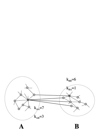
Figure 1: Two connected B-A networks. A few nodes from each network are shown. The intra-network degrees $k_{AA}$ and $k_{BB}$ as well as inter-network degrees $k_{AB}$ and $k_{BB}$ for two sample nodes are presented.

The B-A model is a model of a growing network barabasi . One starts with $m$ fully connected nodes, and adds new nodes to the network. Each new node creates $m$ connections to the extisting network. The probability that a connection will be made to a node $i$ is proportional to its degree $k_{i}$. This results in a scale-free network, with a degree distribution $P(k)\sim k^{-3}$.
We assume that two B-A networks are connected by $E_{AB}$ links (Fig.1). Each of these links connects a node in network $A$ with a node in network $B$. The chance to choose a given node as the end of the inter-network link is proportional to the intra-network node degree. This means that for a small number of links $E_{AB}$, an inter-network degree $k_{AB}$ of a node in the network $A$ is proportional to a intra-network node degree $k_{AA}$. A similar relation holds for degrees in the network $B$.

III Analytic calculations

The problem of the Ising model in a single B-A network was already solved analytically by Bianconi by an appropriately tailored mean-field approach bianconi . We use a similar approach for the problem of two connected networks.
The Hamiltonian of the Ising model for a single B-A network can be written as

$$H=-\sum_{i,j}J_{ij}s_{i}s_{j}-\sum_{i}h_{i}s_{i}$$ (1)

where $s_{i},s_{j}=\pm 1$ are spins of nodes $i,j$, a constant $J_{ij}$ is a ferromagnetic coupling between them and $h_{i}$ is an external field acting on spin $i$. The coupling constants $J_{ij}$ equal to a positive constant if spins are connected, and are zero otherwise.

The exact solution for the average spin $\left\langle s_{i}\right\rangle$ in a single network can be written as

$$\left\langle s_{i}\right\rangle=\left\langle\tanh\left(\beta\sum_{j}J_{ij}s_{j}+\beta h_{i}\right)\right\rangle$$ (2)

where $\beta=1/T$, the temperature $T$ is measured in units of inverse Boltzmann constant $1/k_{B}$ and averaging is over the canonical ensemble. If we now consider an average over all possible realizations of B-A networks, then $\left\langle J_{ij}\right\rangle=Jk_{i}k_{j}/E$. We use the mean field approximation, taking $\left\langle J_{ij}\right\rangle$ in place of $J_{ij}$ in our equation. Since $i$ and $j$ are ordered pairs, the total number of pairs $E$ is twice the number of edges in the network. If we take the external field $h_{i}$ equal to zero, the Eq. 1 has the following form

$$\left\langle s_{i}\right\rangle=\left\langle\tanh\left(\beta J\sum_{j}\left(\frac{k_{i}k_{j}}{E}s_{j}\right)\right)\right\rangle$$ (3)

Now we consider a pair of coupled networks A and B. The parameters describing both networks can be split into four groups - two describe internal properties of each network, and two describe network-network interactions. We introduce the following notation: $s_{Ai}$ and $s_{Bi}$ are spins in networks $A$ and $B$, $J_{AA}$, $J_{BB}$ are coupling constants between spins in networks $A$ and $B$ respectively, $J_{AB}=J_{BA}$ are the coupling constants between spins in different networks, $k_{AAi}$ and $k_{BBi}$ are intra-network node degrees, $k_{ABi}$ and $k_{BAi}$ are inter-network node degrees, $E_{AA}$ and $E_{BB}$ are twice the total numbers of all intra-network links in $A$ and $B$, $E_{AB}=E_{BA}$ is the number of links between the networks.

Now we extend the Eq. 3, introducing the influence of the second network. This way we obtain two equations for average spins in every network. Since we are interested in critical properties, where average spins are close to zero, we can approximate the hyperbolic tangent by a linear function and use a standard mean-field approach. As result we get

$$\left\langle s_{Ai}\right\rangle=\beta J_{AA}k_{AAi}\sum_{j}\frac{k_{AAj}\left\langle s_{Aj}\right\rangle}{E_{AA}}+$$

$$\mbox{}+\beta J_{BA}k_{ABi}\sum_{j}\frac{k_{BAj}\left\langle s_{Bj}\right\rangle}{E_{BA}}$$ (4)

$$\left\langle s_{Bi}\right\rangle=\beta J_{BB}k_{BBi}\sum_{j}\frac{k_{BBj}\left\langle s_{Bj}\right\rangle}{E_{BB}}+$$

$$\mbox{}+\beta J_{AB}k_{BAi}\sum_{j}\frac{k_{ABj}\left\langle s_{Aj}\right\rangle}{E_{AB}}$$ (5)

To get a relation for the system critical temperature we need to have a self-consistent equations for order parameter. The case of a single network required introduction of only single weighted spin $S=\sum_{i}k_{i}\left\langle s_{i}\right\rangle/E$, where the $\left\langle s_{i}\right\rangle$ is mean-field average for a given spin $i$. In the case of two connected networks, we need to consider four such weighted spins $S_{AA}$, $S_{BB}$, $S_{AB}$ and $S_{BA}$.

$$S_{AA}=\sum_{i}k_{AAi}\left\langle s_{Ai}\right\rangle/E_{AA}$$ (6)

$$S_{BB}=\sum_{i}k_{BBi}\left\langle s_{Bi}\right\rangle/E_{BB}$$ (7)

$$S_{AB}=\sum_{i}k_{ABi}\left\langle s_{Ai}\right\rangle/E_{AB}$$ (8)

$$S_{BA}=\sum_{i}k_{BAi}\left\langle s_{Bi}\right\rangle/E_{BA}$$ (9)

$S_{AA}$ and $S_{BB}$ hold the same meaning as for a single network, $S_{AB}$ is the mean weighted spin of the network $A$ observed by spins in the network $B$, while $S_{BA}$ is a mean weighted spin of the network $B$ observed by spins in the network $A$.
Eqs.(10-13) were received from Eqs.(4-5) by multiplying by appropriate factors (see Eqs.6-9) and summing over $i$. These four equations contain only four weighted spins as unknown collective variables and are approximate mean-field description of the system close to a critical point. It follows we receive

$$S_{AA}=\beta J_{AA}S_{AA}\sum_{i}\frac{k_{AAi}^{2}}{E_{AA}}+\beta J_{BA}S_{BA}\sum_{i}\frac{k_{ABi}k_{AAi}}{E_{AA}}$$ (10)

$$S_{BB}=\beta J_{BB}S_{BB}\sum_{i}\frac{k_{BBi}^{2}}{E_{BB}}+\beta J_{AB}S_{AB}\sum_{i}\frac{k_{BAi}k_{BBi}}{E_{BB}}$$ (11)

$$S_{AB}=\beta J_{AA}S_{AA}\sum_{i}\frac{k_{AAi}k_{ABi}}{E_{AB}}+\beta J_{BA}S_{BA}\sum_{i}\frac{k_{ABi}^{2}}{E_{AB}}$$ (12)

$$S_{BA}=\beta J_{BB}S_{BB}\sum_{i}\frac{k_{BAi}k_{BBi}}{E_{BA}}+\beta J_{AB}S_{AB}\sum_{i}\frac{k_{BAi}^{2}}{E_{BA}}$$ (13)

If we assume that $k_{ABi}=p_{A}k_{AAi}$ and $k_{BAi}=p_{B}k_{BBi}$, what means that the number of links outside the network is proportional to the number of links within the network, we can greatly simplify our four equations. This can be done when one takes into account the way we create inter-network links in our model.
Using this assumption, we do not need to consider the cross-network weighted spins $S_{AB}$ and $S_{BA}$ as they are proportional to $S_{AA}$ and $S_{BB}$. Now our first two equations become

$$S_{A}=\beta J_{AA}S_{A}\sum_{i}\frac{k_{AAi}^{2}}{E_{AA}}+\beta J_{BA}S_{B}\sum_{i}\frac{k_{AAi}^{2}p_{A}}{E_{AA}}$$ (14)

$$S_{B}=\beta J_{BB}S_{B}\sum_{i}\frac{k_{BBi}^{2}}{E_{BB}}+\beta J_{AB}S_{A}\sum_{i}\frac{k_{BBi}^{2}p_{B}}{E_{BB}}$$ (15)

where $S_{A}\equiv S_{AA}$ and $S_{B}\equiv S_{BB}$. The equation array can be written as a single matrix equation.

$$\mathbf{S}=\beta\hat{\Lambda}\mathbf{S}$$ (16)

where $\mathbf{S}$ is a vector $\left[\begin{array}[]{c}S_{A}\\ S_{B}\end{array}\right]$ describing the state of the system and $\hat{\Lambda}$ is a matrix describing effective interaction strengths between spins belonging to the same or to different networks

$$\hat{\Lambda}=\left[\begin{array}[]{cc}\Lambda_{AA}&\Lambda_{BA}\\ \Lambda_{AB}&\Lambda_{BB}\\ \end{array}\right]=\left[\begin{array}[]{cc}J_{AA}\frac{\left\langle k_{AA}^{2}\right\rangle}{\left\langle k_{AA}\right\rangle}&p_{B}J_{BA}\frac{\left\langle k_{BB}^{2}\right\rangle}{\left\langle k_{BB}\right\rangle}\\ p_{A}J_{AB}\frac{\left\langle k_{AA}^{2}\right\rangle}{\left\langle k_{AA}\right\rangle}&J_{BB}\frac{\left\langle k_{BB}^{2}\right\rangle}{\left\langle k_{BB}\right\rangle}\\ \end{array}\right].$$ (17)

In the case of a single network A, solutions other than $S_{A}=0$ can exist only if $\beta J_{AA}\frac{\left\langle k_{AA}^{2}\right\rangle}{\left\langle k_{AA}\right\rangle}>1$ bianconi . In the case of two coupled networks, this condition corresponds to an eigenvalue of Eq.16 greater than $1$. The eigenvalues are

$$\lambda_{\pm}=\frac{\beta}{2}\left(\Lambda_{AA}+\Lambda_{BB}\pm\sqrt{\left(\Lambda_{AA}-\Lambda_{BB}\right)^{2}+4\Lambda_{BA}\Lambda_{AB}}\right)$$ (18)

Comparing these eigenvalues with $1$, we get the following critical temperatures

$$T_{c\pm}=\frac{\Lambda_{AA}+\Lambda_{BB}\pm\sqrt{\left(\Lambda_{AA}-\Lambda_{BB}\right)^{2}+4\Lambda_{BA}\Lambda_{AB}}}{2}$$ (19)

Since the diagonal elements of $\hat{\Lambda}$, $\Lambda_{AA}$ and $\Lambda_{BB}$ are critical temperatures $T_{cA}$,$T_{cB}$ for separate networks we can write the critical temperatures for the coupled system as

$$T_{c\pm}=\frac{T_{cA}+T_{cB}\pm\sqrt{\left(T_{cA}-T_{cB}\right)^{2}+4\Lambda_{BA}\Lambda_{AB}}}{2}$$ (20)

To better understand the meaning of these solutions, we introduce the following variables

$$\mathcal{A}=(T_{cA}+T_{cB})/2$$ (21)

$$\mathcal{D}=(T_{cA}-T_{cB})/2$$ (22)

$$\mathcal{C}=\sqrt{\Lambda_{BA}\Lambda_{AB}}$$ (23)

The value $\mathcal{A}$ (”average”) describes an average critical temperatures of the networks, $\mathcal{D}$ (”difference”) is the difference between critical temperatures of both networks, $\mathcal{C}$ (”coupling”) describes a strength of internetwork interactions.

Using this notation the critical temperatures can be written shortly as

$$T_{c\pm}=\mathcal{A}\pm\sqrt{\mathcal{D}^{2}+\mathcal{C}^{2}}$$ (24)

Let us now consider eigenvectors associated with $\lambda_{\pm}$. They are proportional to the magnetization of both networks that appears below a given critical temperature and disappears above it. The unnormalized eigenvectors are

$$\mathbf{S}_{\pm}=\left[\begin{array}[]{c}1\\ \frac{-\mathcal{D}\pm\sqrt{\mathcal{D}^{2}+\mathcal{C}^{2}}}{\Lambda_{BA}}\end{array}\right]$$ (25)

The eigenvector $\mathbf{S}_{-}$ has opposite signs of its components and corresponds to networks ordered with antiparallel weighted spins, while the eigenvector $\mathbf{S}_{+}$ has the same signs of the components and corresponds to networks ordered with parallel weighted spins.
In the limit of vanishing internetwork coupling ($\mathcal{C}=0$) the eigenvalues are simply the diagonal elements of the matrix $\lambda_{A}=T_{cA}$, $\lambda_{B}=T_{cB}$ and the associated normalized eigenvectors are $\mathbf{S}_{A}=\left[\begin{array}[]{c}1\\ 0\end{array}\right]$, $\mathbf{S}_{B}=\left[\begin{array}[]{c}0\\ 1\end{array}\right]$. This means that in this limit two stable states of the system correspond to the ordering of just one of the networks, and there is no relation between the order in each networks. It shows our approach gives correct results in this specific case.
Now let us investigate the inequality conditions for existence of solutions $\mathbf{S}_{\pm}$. From the condition $\lambda_{\pm}>1$ we have

$$\mathcal{A}-T>\sqrt{\mathcal{D}^{2}+\mathcal{C}^{2}}$$ (26)

$$T-\mathcal{A}<\sqrt{\mathcal{D}^{2}+\mathcal{C}^{2}}$$ (27)

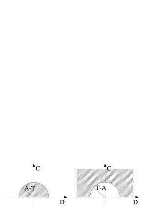
Figure 2: The area of parameters $\mathcal{C}$ and $\mathcal{D}$ where the ordered states $\mathbf{S}_{\pm}$ can exist. The order appears in the dashed areas. The state $\mathbf{S}_{-}$ of antiparallel ordering corresponds to the left picture, the state $\mathbf{S}_{+}$ or parallel ordering corresponds to the right picture. The radius of the circle is the difference $T-\mathcal{A}$. Note that solution $\mathbf{S}_{-}$ does not exist for $\mathcal{A}<T$ and solution $\mathbf{S}_{+}$ exist for any $\mathcal{C}$ and $\mathcal{D}$ for $\mathcal{A}>T$. In the case $\mathcal{C}=0$ the networks do not interact at all, and the solutions lose their normal meaning.

The meaning of these inequalities is presented at Fig.2.
If we consider networks of the same size, the dependence of critical temperatures on inter-network interaction strength $\mathcal{C}$ is linear, and both critical temperatures are the same for $\mathcal{C}\rightarrow 0$. In such case the system critical temperature $\mathcal{T}_{c\pm}=\mathcal{A}=T_{cA}=T_{cB}$ (Fig.3).

The analytic results hold true for any random network, where the probability of a link existing between any two nodes $i$ and $j$ is proportional to the product $k_{i}k_{j}$. This is the only assumption about network structure we have used, so any networks where the condition is fulfilled (i.e. random networks) is described by our analysis.
Our numeric calculations found in the following section, correspond to the specific case of B-A network and constant coupling $J_{AA}=J_{AB}=J_{BA}=J_{BB}=J$. We can write the critical temperatures as follows

$$T_{c\pm}=\frac{T_{cA}+T_{cB}}{2}\pm\sqrt{\left(\frac{T_{cA}-T_{cB}}{2}\right)^{2}+p_{A}p_{B}T_{cA}T_{cB}}$$ (28)

where $T_{cA}=J(m_{A}/2)\ln{N_{A}}$ and $T_{cB}=J(m_{B}/2)\ln{N_{B}}$. The values of $p_{A}$ and $p_{B}$ are not independent, and are connected with the number of links between networks $p_{A}E_{AA}=p_{B}E_{BB}=E_{AB}$.

Figure 3: The dependence of temperatures $T_{c\pm}$ on number of links between networks $E_{AB}$. The dashed lines are analytic predictions (Eq.19). The symbols are numeric results. Circles correspond to $T_{c-}$. Squares and diamonds correspond to $T_{c+}$ and are calculated from susceptibility $\chi=(S_{h}-S_{0})/h$. Triangles correspond to $T_{c+}$ and are calculated from susceptibility $\chi\sim\left\langle S^{2}\right\rangle-\left\langle S\right\rangle^{2}$.

IV Numeric results

Our analytic calculations show the existence of two different ordered states and estimate values of two critical temperatures where these states disappear. Below we investigate numerically a case of two coupled B-A networks with the same number of nodes $N_{A}=N_{B}=5000$ and links $E_{AA}=E_{BB}=40000$ ($m_{A}=m_{B}=5$, $\left\langle k_{AA}\right\rangle=\left\langle k_{BB}\right\rangle=10$).

We run Ising dynamics on these networks, setting the following initial condition: all spins in both networks have the same value $s_{Ai}=s_{Bi}=+1$. We allow the system to relax for $\tau=20$ time steps, perform averaging for $\tau=20$ time steps, then increase the temperature and start from the same initial condition as before. This way, results for different temperatures are not correlated. We find the weighted spin $S=S_{A}+S_{B}$ for each temperature $T$ and average it over $100$ network realizations. Simulations are performed for different numbers of inter-network links $E_{AB}=1000,2000,3000$ and $4000$ that were attached preferentially to fulfill the assumptions of our model (see the discussion at the end of Sect.1).

For low temperatures $T$ the system is ordered. As the temperature increases the average weighted spin $S$ decreases. When the temperatures increase over $T_{c+}$, the ferromagnetic ordered state of both networks disappears, i.e. both networks become paramagnetic (Fig.4).

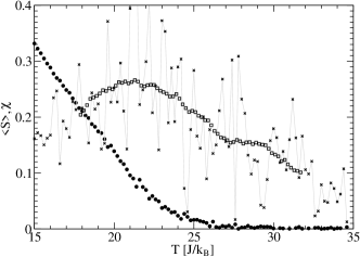
Figure 4: The dependence of the average weighted spin $S=S_{A}+S_{B}$ and its susceptibility for small external field $h=0.05J$ in the case of two B-A networks with $E_{AB}=1000$ connections between them. An initial condition for each temperature is a completely ordered system. The full symbols depict $S$, the X symbols correspond to susceptibility $\chi=\left(S_{0.05}-S_{0}\right)/h$ (the lines are just to guide eye), the empty symbols are 30-point running average of the susceptibility. The parabolic fit was used to find the susceptibility maximum.

Finding the exact value of critical temperature $T_{c+}$ from numerical simulations is not straightforward. If one observes the dependence of the weighted magnetization on rising temperature and tries to fit the magnetization decay to a linear or to an exponential function the results strongly depend on relaxation time $\tau$. To overcome this problem we observed the temperature dependence of the system susceptibility $\chi$. In fact, by comparison to standard models of magnetic systems, one can expect that the initial susceptibility diverges at $T=T_{c+}$. In our finite system we are looking simply for the maximum of $\chi$. To estimate $\chi$ we are using two methods. First we compare average weighted spin $S$ for a small external field $h=0.05J$ and the value of $S_{0}$ with no external field. It follows $\chi=\left(S_{h}-S_{0}\right)/h$. Because such results are strongly fluctuating as a function of system history and temperature (Fig.4), we calculate running average over $30$ temperature points and find the maximum of $\chi$ by fitting a parabolic curve. The top of the parabola corresponds to the position of the critical temperature $T_{c+}$. We found that these values are independent on the relaxation time $\tau$ used in our numerical experiment. The second method of finding the critical temperature $T_{c+}$ is observation of the time average $\left\langle S^{2}\right\rangle-\left\langle S\right\rangle^{2}$, where we average over one relaxation period $\tau$. The magnitude of the fluctuations is proportional to the suceptibility $\chi\sim\left\langle S^{2}\right\rangle-\left\langle S\right\rangle^{2}$ according to the fluctuation-dissipation theorem flucdis . Similarly to previous method, we calculate running average over $10$ points and find the maximum. The values are shifted by a constant value comparing to analytic results and do not fluctuate as much as those obtained from the first method (see Fig.3).

Now we consider the same networks with the following initial condition for each temperature: spins in both networks are ordered antiparallel $s_{Ai}=+1,s_{Bi}=-1$. The relaxation algorithm and the measurement procedure is the same as for parallel spin case, however now we consider absolute values of weighted spin of the whole system $\left|S\right|=\left|S_{A}+S_{B}\right|$. For low temperatures $T$ both networks remain ordered in opposite directions (Fig.5) and as result an average weighted spin value $\left|S\right|=\left|S_{A}+S_{B}\right|$ fluctuates around $0$. When the temperature increases over $T_{c-}$, the state of antiparallely ordered networks disappears and networks start to order in a parallel fashion. An example of such a scenario is presented at Fig.6. When temperature further increases and $T>T_{c+}$ the system becomes paramagnetic.

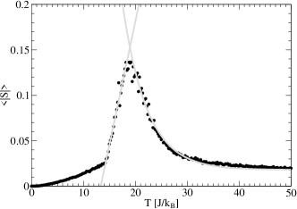
Figure 5: The temperature dependence of the average weighted spin value $\left|S\right|=\left|S_{A}+S_{B}\right|$ in the case of two B-A networks with $E_{AB}=4000$ connections between them. Initial conditions for each temperature are two fully ordered networks with opposite spins. The symbols correspond to numerical data and grey lines are approximations of magnetization behavior below and above critical temperature.

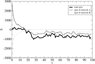
Figure 6: An example of time evolution of magnetization for two networks of size $N_{A}=N_{B}=5000$ and $\left\langle k\right\rangle=4$ with $E_{AB}=500$ links between them in temperature $T=30$ (scaled in $k_{B}/J$). At this temperature, the antiparallel ordered state is not stable, and the initial condition of networks ordered in such fashion evolves towards a stable parallel ordered state.

We found numerically the critical temperature $T_{c-}$ from the intersection of extrapolations of rising and declining part of the curve $S(T)$ (linear fit was used for the rising part and exponential fit for the declining part) (Fig.5). This point slightly depends on relaxation times $\tau$. For large $\tau$ the effect of finite system size can be easily observed and the system jumps from an antiparallel state to a parallel one that has a lower energy.

The results for dependence of $T_{c-}$ and $T_{c+}$ on the number of links between networks $E_{AB}$ agree with the analytic calculations (Fig.3).

V Conclusions

In the system of two B-A network, the Ising model possesses two low-temperature stable states — both networks ordered parallel or antiparallel. It follows there are two critical temperatures corresponding to the disappearance of these two stable states — $T_{c-}$ and $T_{c+}$. They are placed symmetrically around the average of critical temperatures of separate networks. The difference between them depends on density of inter-network links and the difference between critical temperatures of separate networks. The analytic calculations agree with performed numeric simulations.

- (1) A.-L. Barabasi, R. Albert, Science 286, 509 (1999).
- (2) A. Aleksiejuk, J.A. Hołyst, D. Stauffer, Physica A 310, 260-266 (2002).
- (3) G. Bianconi, Phys. Lett. A 303 (2002), 166-168.
- (4) S.N. Dorogovtsev, A.V. Goltsev, J.F.F. Mendes, Phys. Rev. E 66, 016104 (2002).
- (5) A.V. Goltsev, S.N. Dorogovtsev, J.F.F. Mendes, Phys. Rev. E 67, 026123 (2003).
- (6) C.P. Herrero, Phys. Rev. E 69, 067109 (2004).
- (7) B. Tadic, K. Malarz, K. Kulakowski, Phys. Rev. Lett. 94, 137204 (2005).
- (8) M.A. Sumour, M.M. Shabat, Int. J. Mod. Phys. C 16, 585-589 (2005).
- (9) D.H. Kim, G.J. Rodgers, B. Kahng, D. Kim, Phys. Rev. E 71, 056115 (2005).
- (10) J.A. Holyst, K. Kacperski, F. Schweitzer, Physica A 285, 199-210 (2000).
- (11) J.A. Holyst, K. Kacperski, F. Schweitzer, Annual Review of Comput. Phys. 9, 253-273 (2001).
- (12) S. Galam, J. Applied Physics 87, 7040-7042 (2000).
- (13) M. Lewenstein, A. Nowak, B. Latane, Phys. Rev. A 45, 763 (1992).
- (14) M. Girvan, M.E.J. Newman, Proc. Natl. Acad. Sci. USA 99, 7821-7826 (2002).
- (15) D.F. Zheng, G. Ergun, Adv. Complex Systems 6, 507-514 (2003).
- (16) D. Chowdhury, D. Stauffer, Principles of Equilibrium Statistical Mechanics (Wiley-VCH, Berlin, 2000).