CRITICALITY ON NETWORKS WITH TOPOLOGY-DEPENDENT INTERACTIONS

Abstract

Weighted scale-free networks with topology-dependent interactions are studied. It is shown that the possible universality classes of critical behaviour, which are known to depend on topology, can also be explored by tuning the form of the interactions at fixed topology. For a model of opinion formation, simple mean field and scaling arguments show that a mapping $\gamma^{\prime}=(\gamma-\mu)/(1-\mu)$ describes how a shift of the standard exponent $\gamma$ of the degree distribution can absorb the effect of degree-dependent pair interactions $J_{ij}\propto(k_{i}k_{j})^{-\mu}$, where $k_{i}$ stands for the degree of vertex $i$. This prediction is verified by extensive numerical investigations using the cavity method and Monte Carlo simulations. The critical temperature of the model is obtained through the Bethe-Peierls approximation and with the replica technique. The mapping can be extended to nonequilibrium models such as those describing the spreading of a disease on a network.

I Introduction

In recent years -2 ; -1 it has become clear that many natural and technological networks are quite different from simple random networks -5 and share several unexpected properties such as a scale-free degree distribution -2 ; -1 , small world connectivity -4 , soft modularity  and so on. Much work has gone into a precise characterisation of these topological properties for a variety of networks as diverse as the internet 101 , metabolic networks in cells 102 or networks of chemical reactions in planetary atmospheres 104 . Nontrivial topology is now established as an essential ingredient of complex systems 103 . This observation naturally raises the question how these structures are formed and grow. A well known mechanism is that of preferential attachment which leads to the Barabási-Albert network with a power-law degree distribution 1 .

Another important question is how the network topology affects physical properties such as collective behaviour, transport quantities, the spreading of a disturbance, … Particular interest has been devoted to the behaviour of the Ising model on a network. Besides being the standard model of (equilibrium) statistical mechanics, the Ising model is also expected to give a simple description of sociological phenomena such as opinion formation 105 . The first studies of this model indicated that on a Barabási-Albert network, the Ising model is always ordered. It was, however, soon realised that a finite transition temperature can be obtained if one considers the Ising model on scale-free networks with a degree distribution that is less long ranged than that of the Barabási-Albert one 2 ; 3 . Even more interesting is the observation of non-trivial critical behaviour for these cases 2 ; 3 ; 4 ; 5 .

Another mechanism that leads to a finite transition temperature was discovered by one of us in the so called special attention network. This is a model of a weighted network where the interactions between connected spins are made topology-dependent 6 . A further investigation of that and related models then led to the discovery that topology and interaction can be traded’, in the sense that the effect of a change in interaction law can be transformed away by an appropriate change of the degree distribution law. In the present paper we present a detailed investigation of the critical behaviour of the Ising model with degree-dependent interactions. We also discuss the extension of our results to nonequilibrium situations. A summary of our results was published earlier 0p .

This paper is organised as follows. In the next section, we define the model and present the results of a simple mean field theory. In section 3, we study the model with the cavity approach. In section 4, we describe the application of the Bethe-Peierls method and the replica technique to our model. In section 5, we present the results of extensive Monte Carlo simulations. In section 6, we discuss the extension of our main result to a nonequilibrium process. Finally, we present our conclusions in section 7.

II The model

Our model can be defined on a general network (or graph). When in a graph a vertex (or node) $i$ is connected with $k_{i}$ other nodes we say it has degree $k_{i}$. We will mostly have in mind a scale-free network for which the degree is a random variable whose distribution $P(k)$ is a power-law: $P(k)\propto k^{-\gamma}$. We take $\gamma>2$ so that the average degree $Q=\int kP(k)dk$ is finite. For future reference we also introduce the notation $Q_{2}$ for the second moment of $P(k)$. The Barabási-Albert (BA) network has $\gamma=3$ 1 . The number of nodes in the network is denoted by $N$.

We next define an Ising model on this network by associating to each node $i$ a variable $s_{i}=\pm 1$ and to each pair of linked nodes an energy $-J_{ij}s_{i}s_{j}$. In this paper, we will choose the couplings $J_{ij}$ to be given by

$$J_{ij}=JQ^{2\mu}/(k_{i}k_{j})^{\mu}\,.$$ (1)

with $J>0$. For $\mu=0$, the behaviour of this model has been investigated by various authors and the critical behaviour was found to depend on $\gamma$ 2 ; 3 ; 4 ; 5 . For $\gamma>5$ the results of standard mean field theory were found to apply: the critical temperature $T_{c}$ is finite, the order parameter vanishes with an exponent $1/2$ and the specific heat has a finite jump at $T_{c}$. When $3<\gamma<5$, the transition temperature remains finite, the specific heat goes to zero continuously as a function of temperature with an exponent that depends on $\gamma$. The same is true for the order parameter. In the borderline case $\gamma=5$, logarithmic corrections appear. For all cases with $\gamma>3$, the zero-field susceptibility diverges as $|T-T_{c}|^{-1}$. Finally, when $2<\gamma\leq 3$, the system is ordered at all temperatures.

When $\mu=1/2$, our model corresponds to the special attention network (SAN) introduced earlier by one of us 6 . A simple mean field approach showed that on a BA network, the SAN has a finite transition temperature 6 . We start by extending that simple approach to the case of general $\mu$ and $\gamma$.

II.1 A simple mean-field approximation

For a given network realization, the local magnetisation $m_{i}=\langle s_{i}\rangle$ at node $i$ obeys the exact equation

$$m_{i}=\langle s_{i}\rangle=\left\langle\tanh\left(\sum_{j=1}^{k_{i}}\frac{J_{ij}}{k_{B}T}s_{j}\right)\right\rangle\,.$$ (2)

Here $\langle.\rangle$ is the thermal average, $k_{B}$ is Boltzmann’s constant and $T$ is the temperature. Following Bianconi 7 , we now apply a double mean field approximation to this equation by rewriting it as

$$m_{i}=\tanh\left(\sum_{j=1}^{N}\frac{[J_{ij}]}{k_{B}T}m_{j}\right)\,,$$ (3)

where the sum now runs over all the nodes and $[.]$ denotes the average over all the realisations of the network with a fixed set of degrees $\{k_{i}\}$. For a BA network the probability $p_{ij}$ that two nodes are connected was shown to be equal to $k_{i}k_{j}/(QN)$, 7 and we can expect this result to hold in some other cases 5 . We therefore have

$$[J_{ij}]=J_{ij}p_{ij}=\frac{JQ^{2\mu-1}}{N}\left(k_{i}k_{j}\right)^{1-\mu}\,,$$ (4)

so that Eq. (3) can be rewritten as

$$m_{i}=\tanh\left(\frac{JQ^{\mu}}{k_{B}T}\ k_{i}^{1-\mu}\frac{Q^{\mu-1}}{N}\sum_{j=1}^{N}k_{j}^{1-\mu}m_{j}\right)\,.$$ (5)

The quantity

$$S=\frac{Q^{\mu-1}}{N}\sum_{j=1}^{N}k_{j}^{1-\mu}m_{j}\,,$$ (6)

is a convenient order parameter. From Eq. (5) it follows that $S$ obeys the selfconsistency equation

$$S=\frac{Q^{\mu-1}}{N}\sum_{i=1}^{N}k_{i}^{1-\mu}\tanh\left(\frac{JQ^{\mu}}{k_{B}T}k_{i}^{1-\mu}S\right)$$ (7)

For $N\to\infty$, the term on the right hand side is simply related to the average over the distribution $P(k)$ so that we can rewrite Eq. (7) as

$$S=Q^{\mu-1}\int_{m}^{\infty}k^{1-\mu}\tanh\left(\frac{JQ^{\mu}}{k_{B}T}k^{1-\mu}S\right)P(k)dk$$ (8)

Here $m\geq 1$ is the lowest degree that is possible in the network. Eq. (8) can be analysed in a standard way. For example, the critical temperature is determined by assuming $S$ to be small. After linearisation we then obtain

$$T_{c}=\frac{JQ^{2\mu-1}}{k_{B}}\int_{m}^{\infty}k^{2-2\mu}P(k)dk\,.$$ (9)

For the power-law distribution this gives a finite $T_{c}$ provided $\gamma>3-2\mu$. This is consistent with the earlier finding of a finite $T_{c}$ for the SAN on the BA network. One could then go on and determine, for example, the exponent $\beta$ from a further analysis of Eq. (8). It is however more suitable to perform the transformation of variables

$$k^{\prime}=Q^{\mu}k^{1-\mu}$$ (10)

This gives for the case that the degree distribution is power-law, and for $\mu<1$

$$S=A\int_{m^{\prime}}^{\infty}\left(k^{\prime}\right)^{\frac{1-\gamma}{1-\mu}}\tanh\left(\frac{Jk^{\prime}S}{k_{B}T}\right)dk^{\prime}$$ (11)

where $A$ is a constant and $m^{\prime}=Q^{\mu}m^{1-\mu}$. Comparison with (8) teaches us that (11) is precisely the mean field equation for $\mu^{\prime}=0$ and for a degree distribution with an exponent that is modified to

$$\gamma^{\prime}=\frac{\gamma-\mu}{1-\mu}$$ (12)

This relation can be expected to hold more generally. Indeed, it should be valid whenever within a mean-field approach the degree $k$ only enters in physical properties through the quenched average interaction between any two nodes with fixed degrees, $k_{i}$ and $k_{j}$. This average is, as shown above, $J_{ij}p_{ij}$ with $p_{ij}=k_{i}k_{j}/(QN)$. For $\mu\neq 0$, the $k_{i}$ can then be transformed using (10). In order to retain the same physics, averages over the degree distribution must be invariant. This requires a distribution transformation

$$P(k)=P^{\prime}(k^{\prime}(k))\frac{dk^{\prime}(k)}{dk}$$ (13)

from which (12) follows for a scale-free $P(k)$. In section 6, we will in fact show that (12) also holds for a contact process with degree-dependent infection rates. The general derivation scheme outlined above, will also apply there. Thus, our simple mean field analysis indicates that by tuning $\mu\in[2-\gamma,1]$ we can encounter the whole range of universality classes that was found in earlier work at $\mu=0$. As an example, one can study the whole set of universality classes by working on a BA-network and tuning $\mu$. For the particular example of the SAN, (12) gives $\gamma^{\prime}=5$.

In the rest of this paper we will apply several other approaches that go beyond simple mean field to our model. These will allow us to get a better estimate than (9) for the critical temperature, and to verify the equivalence between universality classes as expressed in Eq. (12).

We also observe that from (5) and (6) it follows that

$$m_{i}=\tanh\left(\frac{JQ^{\mu}}{k_{B}T}k_{i}^{1-\mu}S\right)\approx\frac{JQ^{\mu}}{k_{B}T}k_{i}^{1-\mu}S$$ (14)

where the last approximation holds close to $T_{c}$. We therefore anticipate that the local magnetisation is proportional to $k_{i}^{1-\mu}$, a result that we will use further in this paper and which will be verified numerically.

III The cavity method

We begin with a study of our model using the cavity approach. One reason for this is that concepts like the cavity field and the propagated field, which also appear in the replica study of our model, can be introduced in a physically transparent way within the context of this method.

The cavity method is closely related to the well known Bethe-Peierls (BP) approximation for a spin model on a Cayley tree 11 . In fact, both methods are equivalent when there is replica symmetry (for the precise relation between various mean-field approximations, see reference 20). The cavity method was applied to diluted spin models in references 21-23. For Ising like models on a network, the method has the advantage that it can take into account site degree correlations, which certainly are present in networks grown via a preferential attachment rule 12 ; 13 or in real world networks (from biology, sociology, information technology, …). These correlations can be measured in terms of the clustering coefficient, the betweenness -2 or the abundance of cycles of a given length 14 ; 15 . This has to be contrasted with the replica approach of the next section, which, in its simplest form assumes independence of the site degrees. Extensions of the replica approach that take into account degree correlations are known 13 , but necessarily are more involved. Another attractive property of the cavity method is that thermodynamic quantities like the magnetisation can be calculated on a single network realisation. Together these properties allow the analysis of real world networks and to work with ensembles that, as in the BA case, are defined only through a growth process.

To derive the cavity equations, it is assumed that the network has the structure of a tree. It is at first sight paradoxical that the tree approximation is adequate for determining the critical point of the network, because the Ising model on a tree (without loops) cannot display spontaneous symmetry breaking (SSB) at finite temperature and thus $T_{c}=0$. However, in the same way that the Bethe-Peierls approximation for an Ising model on a Cayley tree introduces an effective symmetry breaking field in the bulk so that SSB becomes possible, the cavity method introduces a random distribution of effective fields in the bulk (all fields being of the same sign) so that SSB becomes possible notwithstanding the absence of loops on the tree. Thus, the SSB due to the sparse loops in the actual network is replaced, in the cavity method, by the SSB due to the effective fields. The question remains whether the two SSB mechanisms lead to exactly the same value of $T_{c}$.

Consider then a particular site $j$ in the network (see Fig. 1). The assumption of tree structure implies that the sites connected to $j$ form the roots of a set of independent subgraphs.

Figure 1: Local structure of a network used in the derivation of the cavity equations (see text).

The site $j$ is connected to $k_{j}$ others. In the presence of an external field $H$ the magnetisation at site $j$ is given by (with $\beta=1/k_{B}T$)

$$m_{j}=\frac{e^{\beta H}\prod_{i=1}^{k_{j}}Z_{ij}(+)-e^{-\beta H}\prod_{i=1}^{k_{j}}Z_{ij}(-)}{e^{\beta H}\prod_{i=1}^{k_{j}}Z_{ij}(+)+e^{-\beta H}\prod_{i=1}^{k_{j}}Z_{ij}(-)}$$ (15)

Here $Z_{ij}(s)$ is the partition sum of the whole subgraph starting from site $i$, and $s$ is the value of the spin at $j$. This partition sum also includes the bond between the vertices $i$ and $j$. Clearly, we can always write

$$Z_{ij}(s)\propto e^{\beta u_{ij}s}$$ (16)

where we call $u_{ij}$ the local cavity message. With this assumption, Eq. (15) becomes

$$m_{j}=\tanh\left(\beta H+\beta\sum_{i=1}^{k_{j}}u_{ij}\right)$$ (17)

which also gives a clear physical interpretation to $u_{ij}$. Indeed, $u_{ij}$ can be seen as the contribution to the total magnetic field acting on site $j$ coming from the independent subtree having site $i$ as root. In the cavity ansatz, those local contributions are indeed independent. We need extra equations to determine the cavity fields selfconsistently. In order to determine these, we write $Z_{ij}(s)$ in terms of the subtrees that are connected to it (see Fig. 1). We denote the sites adjacent to $i$ by the index $l$. Their number equals $k_{i}$, but clearly, one of them is the starting site $j$. From the definition of $Z_{ij}(s)$, we have

$$Z_{ij}(s)=e^{\beta H+\beta J_{ij}s}\prod_{l=1}^{k_{i}-1}Z_{li}(+)+e^{-\beta H-\beta J_{ij}s}\prod_{l=1}^{k_{i}-1}Z_{li}(-)$$ (18)

so that using Eq. (15) and Eq. (16), we obtain after a little algebra

$$u_{ij}=\frac{1}{\beta}\tanh^{-1}\left(\tanh\left(\beta h_{ij}\right)\tanh\left(\beta J_{ij}\right)\right)$$ (19)

where

$$h_{ij}=H+\sum_{l=1}^{k_{i}-1}u_{li}$$ (20)

is called the propagated field (sometimes also called cavity field). The equations (19) -(20) are known as belief propagation equations 11 . They were derived iteratively here, but it is possible to obtain the same equations through a variational procedure and assuming that configuration probabilities properly factorize on a tree. A short derivation from the variational approach will be presented in section 4.1.

We solved the belief propagation equations iteratively for different values of $\mu$ in our model. One can show in this case that belief propagation equations, when converging, do so to a unique fixed point (beside the fully paramagnetic solution which is always present in absence of external field). When possible, we could also be interested in averaging belief propagation equations over a proper random network ensemble. In that case, equations for propagated messages and fields become a set of integral equations for field probability distributions 9 ; 10 . This unfortunately cannot be easily done in the case of growing network ensembles, like the BA one. In the case of uncorrelated power-law degree distributed graphs, the self consistent integral equations can be written straightforwardly from (19) and (20). The resulting equations turn out to be exactly equations (48) and (49) that we will obtain through the replica approach. On the same random network ensemble, the replica symmetric calculation and the cavity method are therefore completely equivalent. Note, however, that the analytical results for $T_{c}$ presented in the replica calculation are valid for a graph ensemble which is not exactly the BA one. It is therefore plausible that we obtain a slight discrepancy between the replica and the cavity results obtained after averaging over real BA network realisations.

Within the cavity approach, it is also possible to obtain the free energy $F(\beta)$ and from this other thermodynamic quantities such as the energy $U(\beta)$ and the specific heat $C(\beta)$. Here we only quote the result for $U$

$$U(\beta)=-\sum_{i,j}J_{ij}\left(\frac{\tanh(\beta J_{ij})+\tanh(\beta h_{ij})\tanh(\beta h_{ji})}{1+\tanh(\beta J_{ij})\tanh(\beta h_{ij})\tanh(\beta h_{ji})}\right)$$ (21)

We now turn to a discussion of our numerical results. These were obtained on BA networks. Ensemble averages in the case of BA networks can be performed numerically generating a large number of graphs with a given number of nodes with the usual preferential attachment rule, and subsequently averaging the results over all the graphs at a given $N$. Quantities such as $T_{c}$ and the critical exponents can then be found using finite size scaling. We studied $1000$ realisations of networks of $N=50,100,250,500,1000,5000$ and $10^{4}$ nodes, $100$ realisations with $N=5\times 10^{4}$ nodes and $10$ realisations of $10^{5}$ and $10^{6}$ nodes. For each of these the cavity messages were determined iteratively. The numerical results showed little fluctuations when comparing different realisations, even for small network sizes.

We first investigated the SAN and studied cases with $Q=4,6,8,10$ and $20$. In table 1 (see section 4) we give our estimates for $T_{c}$ as a function of $Q$. These results will be compared with those coming from other methods.

From the behaviour of the magnetisation $M$ ($M=\frac{1}{N}\sum_{i}m_{i}$) below $T_{c}$ (Fig. 2), we can determine the exponent $\beta$. We find a value which is very close to the mean field value of $1/2$. This value hardly depends on $N$ or on $Q$. These data also allow us to obtain finite size estimates $T_{c}(N)$ for the critical temperature. We measured the magnetisation within a small temperature window around each value of $T_{c}(N)$ and this for small values of the external field $H$. From an extrapolation for large $N$, the value of the exponent $\delta$ was found to be close to $3$. More precisely we find $1/\delta=0.333\pm 0.010$ for $Q=4$. For bigger $Q$-values, we find the same value for $1/\delta$ while the error decreases with $Q$. Using the scaling relation $\gamma_{s}=\beta(\delta-1)$, this leads to the value $1$ for the susceptibility exponent $\gamma_{s}$.

Figure 2: Magnetisation versus temperature for $Q=4$ (left) and $Q=10$ (right) for $N=10^{2},10^{3},10^{4},10^{5}$. For $Q=4$, results for $N=10^{6}$ are also included.

Specific heat computations (see Fig. 3) show a jump around the transition. However, the discontinuity seems to become smaller for large $N$ such that

$$\lim_{T\to T_{c}^{-}}\frac{dC}{dT}=-\infty$$ (22)

Both cases (vanishing jump with diverging derivative or discontinuity in $C$) can be consistent with a critical exponent $\alpha=0$.

The conjecture embodied in (12) predicts that the SAN on a BA network has $\gamma^{\prime}=5$. The critical exponents are then given by $\gamma_{s}=1$, $\beta=1/2$ and $\alpha=0$ 2 ; 3 ; 4 . In conclusion, we can say that the results from the cavity method for the SAN are in agreement with the relation (12).

Figure 3: Specific heat versus temperature for $Q=4$ (left) and $Q=10$ (right) for $N=10^{2},10^{3},10^{4},10^{5}$. For $Q=4$, results for $N=10^{6}$ are also included.

A peculiar behaviour of the specific heat can be seen in Fig. 3. For both $Q$-values shown there, one observes a maximum in the specific heat at a temperature below the critical one. This seems not to be a finite size effect. Moreover, as Fig. 4 shows, this kind of behaviour does not appear for the SAN on a network with a Poisson degree distribution.

Figure 4: Specific heat versus temperature for a graph with a degree distribution that is Poisson ($Q\approx 4$). The plots refer to an average over 500 realisations for $N=10^{3},10^{4}$ and 50 realisations for $N=10^{5}$.

Another interesting feature is that close to $T_{c}$ we observe an inversion phenomenon in the local magnetisation of sites. Below the transition, there is a clear hierarchy in sites according to their spin magnetisation. Even though couplings are weighted, hubs are still the most magnetized sites and are believed to drive the transition. Plots of the local magnetization versus site degree for a few values of the temperature above and below $T_{c}$ are shown in Fig. 5. These data are consistent with the prediction (14) coming from the simple mean field theory.

Figure 5: Scatter plot of single node magnetisations versus degree for one network of $N=10000$ and $Q=4$ at different temperatures: (a) below $T_{c}(k_{B}T_{c}/J=2.87\pm 0.01)$, (b) above $T_{c}$.

As can be seen in the scatter plots of Fig. 6, low degree nodes connected to hubs have a lower magnetisation than equal degree nodes that are not connected to hubs. Above the transition, however, this situation is reversed. This is different from the situation for an Ising model with degree-independent couplings on a network, where at fixed degree, nodes connected to hubs are always most magnetised.

Figure 6: Scatter plot of magnetisations of all nodes of degree $k=2$ for the same network as in Fig. 5, versus node index (i.e. the time step at which this node is added when the network grows according to the BA-rule). Diamonds represent those nodes connected to hubs whereas crosses represent nodes of degree 2 not connected to hubs. Older nodes (smaller index) are on average more connected to hubs than later ones. Different clusters represent different temperatures. In (a) we show the results for two temperatures below $T_{c}$ while in (b) the temperatures are above the critical one. The inversion phenomenon described in the text can clearly be seen.

Besides the SAN, we also investigated our model with the same techniques for $\mu=1/3$ on a BA network. For that case, (12) predicts $\gamma^{\prime}=4$ which leads to the exponent values $\gamma_{s}=\beta=-\alpha=1$ and $\delta=2$. In Fig. 7 we show some representative results for the specific heat and the magnetisation as a function of temperature (both at $Q=4$). They show the appearance with increasing $N$ of a regime where both quantities depend linearly on temperature, consistent with the above prediction.

Figure 7: The specific heat (left) and the magnetisation (right) as a function of temperature for a BA network with $\mu=1/3$. The average connectivity is $Q=4$.

IV The critical temperature

In this section we discuss two approaches, the Bethe-Peierls approximation and the replica method, that allow us to get precise results for the critical temperature. Both approaches assume that there are no degree correlations present in the network.

IV.1 Bethe-Peierls approximation

The Bethe-Peierls (BP) approximation is the simplest of the cluster variation methods 16 . It amounts to approximating the entropic part of the free energy, $F(\beta)$, by restricting the probability distribution $\rho$ of a configuration of $N$ spins to a combination of single-site and nearest-neighbour pair distributions. For a particular fixed network, this leads to the following expression for $F(\beta)$

$$F(\beta)\beta\approx\beta\langle H\rangle+\sum_{i}(1-k_{i})\sum_{s_{i}=\pm 1}\rho_{i}\ln\rho_{i}+\frac{1}{2}\sum_{i}\sum_{j=1}^{k_{i}}\sum_{s_{i},s_{j}=\pm 1}\rho_{ij}\ln\rho_{ij}$$ (23)

where

$$H = -\frac{1}{2}\sum_{i}\sum_{j=1}^{k_{i}}J_{ij}s_{i}s_{j}$$ (24)

$$\rho_{i} = \frac{1+m_{i}s_{i}}{2}$$ (25)

$$\rho_{ij} = \frac{1+m_{i}s_{i}+m_{j}s_{j}+\psi_{ij}s_{i}s_{j}}{4}$$ (26)

Here $\psi_{ij}=\langle s_{i}s_{j}\rangle$. Expressions for the local magnetisations $m_{i}$ and the neighbour spin-spin correlations $\psi_{ij}$ are obtained by looking for extrema of the free energy

$$\frac{\partial F}{\partial m_{i}} = 0\ \ \ \ \ \ \ \ \forall\ i$$ (27)

$$\frac{\partial F}{\partial\psi_{ij}} = 0\ \ \ \ \ \ \ \ \forall\ i,j$$ (28)

It can be shown that (27) and (28) are fully equivalent to (19) and (20) 11 .

Next, the resulting selfconsistency equations are linearised in the $m_{i}$. In this way one obtains for the spin-spin correlations

$$\psi_{ij}=\tanh{(J_{ij}/k_{B}T)}$$ (29)

After summing over all the vertices, the equation for the magnetisation becomes

$$\frac{1}{N}\sum_{r}(k_{r}-1)m_{r}=\frac{1}{N}\sum_{r}m_{r}\sum_{j=1}^{k_{r}}\frac{1}{1+\psi_{rj}}$$ (30)

Since we now want to get a simpler analytic expression for the critical temperature, we do not solve (30) on single graphs, as already done in a more complete setting with the cavity approach. Instead, we average it over the network realizations. This we do in two steps. Firstly, using a similar approximation as in section 2.1, we replace the second sum on the right hand side by a sum over all nodes. Hence, we obtain

$$\frac{1}{N}\sum_{r}(k_{r}-1)m_{r}=\frac{1}{N}\sum_{r}m_{r}\sum_{j=1}^{N}p_{rj}\left(\frac{1}{1+\psi_{rj}}\right)$$ (31)

where again $p_{rj}=k_{r}k_{j}/(QN)$. Secondly, we insert the proportionality between $m_{j}$ and $k_{j}^{1-\mu}$ implied by (14): $m_{j}\propto k_{j}^{1-\mu}$. In the limit $N\to\infty$ the resulting equation can again be written in terms of the average over the degree distribution. We then finally obtain

$$Q\sum_{k=m}^{\infty}P(k)(k-1)k^{1-\mu}=\sum_{k_{1}=m}^{\infty}P(k_{1})k_{1}^{2-\mu}\sum_{k_{2}=m}^{\infty}P(k_{2})\frac{k_{2}}{1+\tanh\left(\frac{JQ^{2\mu}}{k_{B}Tk_{1}^{\mu}k_{2}^{\mu}}\right)}$$ (32)

For the case $\mu=0$, and for $Q$ large, (32) can be approximated and gives the estimate $k_{B}T_{c}/J\approx(Q_{2}-Q)/Q$, in agreement with exact results 2 . Also, for the SAN on a BA-network, we get for $Q$ large: $k_{B}T_{c}/J\approx Q-1$. On a regular lattice with coordination number $Q$, the Bethe-Peierls approximation gives $J/(k_{B}T_{c})=\ln{\left(\frac{Q}{Q-2}\right)}/2$ 777 . As can be seen in table 1, this approximation gives a very good value for $T_{c}$ for $Q>4$.

Equation (32) can be solved numerically. In table 1 we present our results for the SAN on a BA network with $P(k)=2m(m+1)/k(k+1)(k+2)$ (for this case, $m=Q/2$).

Table 1: Critical temperature $k_{B}T_{c}/J$ as a function of $Q$ for the SAN on networks, as obtained from various approaches. On a regular lattice with coordination number $Q$, the Bethe-Peierls (BP) approximation gives $J/k_{B}T_{c}=\ln\left(Q/(Q-2)\right)/2$. This value is given in the second column. In the third column the results of the cavity approach are given, while the fourth column presents the estimate obtained within the Bethe-Peierls approximation on the network, equation (32). The fifth column gives the solution to (56) obtained in the replica approach. The last column gives the estimates coming from the Monte Carlo simulations. The results for the cavity method and the simulations were obtained on BA networks. The results for the network BP and the replica method were obtained on uncorrelated networks. This has dramatic consequences for $Q=2$. For $Q=2,T_{c}=0$ on BA networks because BA networks with $Q=2$ are simple trees without loops. In contrast, uncorrelated networks with $Q=2$ may feature loops as well as disconnected parts.

$Q$ lattice BP cavity network BP replica Monte Carlo 2 0. 0. 0.95230 0.94614 0. 4 2.8854 2.87$\pm$ 0.01 2.95508 2.92468 2.91 $\pm$ 0.02 6 4.9326 4.92$\pm$ 0.01 4.9554 4.94511 8 6.9521 6.94$\pm$ 0.01 6.9406 6.95796 10 8.9628 8.94$\pm$ 0.01 8.9087 8.96607 8.96 $\pm$ 0.01 20 18.9824 18.98 $\pm$ 0.01 18.9107 18.98187 19.09 $\pm$ 0.04

IV.2 Replica theory for an uncorrelated network

The replica approach is a powerful mathematical technique that provides a way to perform an average over random network ensembles. For the present model, and in absence of degree correlations, it leads to a relatively simple analytical equation from which the critical temperature can be determined numerically.

In order to define the random ensemble of networks we start by defining the adjacency matrix $C$ of a graph. This matrix is the $N\times N$ matrix whose element $c_{ij}$ is one if there is a link between node $i$ and $j$ and zero otherwise. Clearly,

$$\sum_{j=1}^{N}c_{ij}=k_{i}$$ (33)

Moreover, for undirected graphs $C$ is symmetric, $c_{ij}=c_{ji}$. Using the adjacency matrix we can write the Hamiltonian ${\cal H}$ for our model as

$${\cal H}=-\frac{1}{2}\sum_{i\neq j}^{N}J\Phi(k_{i},k_{j})c_{ij}s_{i}s_{j}-H\sum_{i=1}^{N}s_{i}$$ (34)

where in our case $\Phi(k_{i},k_{j})=J_{ij}/J=Q^{2\mu}/(k_{i}k_{j})^{\mu}$. The replica approach can, however, be performed for more general forms of $\Phi$. In Eq. (34), we have also included an external magnetic field $H$ for later convenience.

We calculate the typical properties of all networks with a given fixed set of degrees $\{k_{i}\}$. The matrix elements $c_{ij}$ are assumed to be completely uncorrelated apart from the constraint (33). Therefore given that

$$P(c_{ij})=\frac{Q}{N}\delta_{c_{ij},1}+\left(1-\frac{Q}{N}\right)\delta_{c_{ij},0}$$ (35)

we can write their joint probability distribution as

$${\cal P}(\{c_{ij}\})\propto\prod_{i<j}P(c_{ij})\prod_{i}\delta\left(\sum_{j}c_{ij}-k_{i}\right)$$ (36)

As usual in disordered systems, we compute the quenched average of the free energy density per site, $f_{q}(\beta)$, from which typical properties can be determined

$$-\beta f_{q}(\beta)=\lim_{N\to\infty}\frac{1}{N}\left[\ln Z\right]$$ (37)

where $\beta=1/(k_{B}T)$. Since the calculation is rather involved but standard 3 ; 8 ; 17 , we summarize here only the major steps and results. Using the equality $\ln Z=\lim_{n\to 0}\frac{1}{n}(Z^{n}-1)$ the quenched free energy density is written as

$$-\beta f_{q}(\beta)=\lim_{N\to\infty}\lim_{n\to 0}\frac{1}{Nn}\left(\left[Z^{n}(\beta)\right]-1\right)$$ (38)

The replicated partition function $Z^{n}(\beta)$ equals

$$Z^{n}(\beta)=\sum_{\vec{s}_{1}}\cdots\sum_{\vec{s}_{N}}\exp\left[\frac{\beta}{2}\sum_{\alpha=1}^{n}\sum_{i,j}J_{ij}s_{i}^{\alpha}s_{j}^{\alpha}+\beta H\sum_{\alpha=1}^{n}\sum_{i=1}^{N}s_{i}^{\alpha}\right]$$ (39)

where $\vec{s}_{i}=\{s_{i}^{1},\dots,s_{i}^{n}\}$. For the distribution of connectivities given in Eq. (36), the average $\left[\cdot\right]$ is

$$\left[A(\{c_{ij}\})\right]=\frac{1}{{\cal N}}\int\left[\prod_{i<j}dc_{ij}P(c_{ij})\right]\prod_{i=1}^{N}\delta\left(\sum_{j}c_{ij}-k_{i}\right)A(\{c_{ij}\})$$ (40)

where ${\cal N}$ is the normalisation

$${\cal N}=\int\left[\prod_{i<j}dc_{ij}P(c_{ij})\right]\prod_{i=1}^{N}\delta\left(\sum_{j}c_{ij}-k_{i}\right)$$ (41)

In order to calculate this average, it is common to introduce an exponential representation of the constraint

$$\delta\left(\sum_{j=1}^{N}c_{ij}-k_{i}\right)=\int_{0}^{2\pi}\frac{d\xi_{i}}{2\pi}e^{i\xi_{i}\left(\sum_{j=1}^{N}c_{ij}-k_{i}\right)}$$ (42)

A straightforward but lengthy calculation in which we integrate over the disorder and the auxiliary variables $\xi_{i}$ allows us to obtain the free energy density in terms of the functional order parameter

$$R_{k}(\vec{s})=\frac{1}{N}\sum_{i=1}^{N}\delta_{\vec{s},\vec{s}_{i}}\delta_{k,k_{i}}e^{i\xi_{i}}$$ (43)

and its canonical conjugate $\hat{R}_{k}$. This order parameter is an order parameter in the replica space which is the joint density of finding a spin configuration $\vec{s}$ with average connectivity $k$ at each site, when a link has been removed from that site. The result is

$$-\beta f_{q}(\beta)=\mbox{Extr}_{\{\widehat{R}_{k}(\vec{s}),R_{k}(\vec{s})\}}\Bigg{\{}-Q\sum_{\vec{s},k}\widehat{R}_{k}(\vec{s})R_{k}(\vec{s})+\frac{Q}{2}+$$

$$\sum_{k}P(k)\ln\sum_{\vec{s}}\big{[}\widehat{R}_{k}(\vec{s})\big{]}^{k}e^{\beta H\sum_{\alpha=1}^{n}s^{\alpha}}+\frac{Q}{2}\sum_{k,k^{\prime}}\sum_{\vec{s},\vec{\sigma}}R_{k}(\vec{s})R_{k^{\prime}}(\vec{\sigma})e^{\beta J\Phi(k,k^{\prime})\vec{s}\cdot\vec{\sigma}}\Bigg{\}}$$ (44)

where we also performed the rescaling $i\widehat{R}_{k}(\vec{s})\to-Q\widehat{R}_{k}(\vec{s})$.

Stationarity of the free energy with respect to $R_{k}(\vec{s})$ and $\widehat{R}_{k}(\vec{s})$ leads to the saddle-point equations

$$\widehat{R}_{k}(\vec{s}) = \sum_{k^{\prime},\vec{\sigma}}R_{k}^{\prime}(\vec{\sigma})e^{\beta J\Phi(k,k^{\prime})\vec{s}\cdot\vec{\sigma}}$$

$$R_{k}(\vec{s}) = \frac{kP(k)}{Q}\frac{\left[\widehat{R}_{k}(\vec{s})\right]^{k-1}e^{\beta H\sum_{\alpha=1}^{n}s^{\alpha}}}{\sum_{\vec{\sigma}}\left[\widehat{R}_{k}(\vec{\sigma})\right]^{k}e^{\beta H\sum_{\alpha=1}^{n}\sigma^{\alpha}}}$$ (45)

If all the $\Phi(k,k^{\prime})$ are positive, so that the model only has ferromagnetic interactions, it can be expected that the solution to these equations has replica symmetry (RS). For the order parameter and its conjugate, this assumption takes the form

$$R_{k}(\vec{s})=\int dhW_{k}(h)\frac{e^{\beta h\sum_{\alpha=1}^{n}s^{\alpha}}}{\left[2\cosh(\beta h)\right]^{n}}$$ (46)

and

$$\widehat{R}_{k}(\vec{s})=\int duQ_{k}(u)\frac{e^{\beta u\sum_{\alpha=1}^{n}s^{\alpha}}}{\left[2\cosh(\beta u)\right]^{n}}$$ (47)

respectively. Here $h$ and $u$ are the local cavity message and the propagated field that we already encountered in section 2. While the cavity approach calculates these fields for a specific network, in the replica approach we can obtain their probability distributions over the set of all networks obeying the constraints (33). These distributions are denoted as $W_{k}(h)$ and $Q_{k}(u)$ respectively. Within the RS ansatz, the saddle-point equations become

$$Q_{k}(u) = \sum_{k^{\prime}}\int dhW_{k^{\prime}}(h)\delta\left(u-\frac{1}{\beta}\tanh^{-1}\left[\tanh(\beta h)\tanh\left[\beta J\Phi(k,k^{\prime})\right]\right]\right)$$ (48)

$$W_{k}(h) = \frac{P(k)k}{Q}\int\left[\prod_{l=1}^{k-1}du_{l}Q_{k}(u_{l})\right]\delta\left(h-\sum_{l=1}^{k-1}u_{l}-H\right)$$ (49)

and the free energy density equals

$$\beta f_{q}(\beta) = -Q\ln{2}+Q\sum_{k}\int dudhQ_{k}(u)W_{k}(h)\ln\left[1+\tanh(\beta u)\tanh(\beta h)\right]$$

$$- \sum_{k}P(k)\int\left[\prod_{l=1}^{k}du_{l}Q_{k}(u_{l})\right]\ln\left[\frac{2\cosh\left[\beta\left(\sum_{l=1}^{k}u_{l}+H\right)\right]}{\prod_{l=1}^{k}2\cosh\left(\beta u_{l}\right)}\right]$$

$$- \frac{Q}{2}\sum_{k,k^{\prime}}\int dhdh^{\prime}W_{k}(h)W_{k^{\prime}}(h^{\prime})F_{kk^{\prime}}(\beta,h,h^{\prime})$$

where

$$F_{kk^{\prime}}(\beta,h,h^{\prime})=\ln\left[\cosh\left[\beta J\Phi(k,k^{\prime})\right]+\sinh\left[\beta J\Phi(k,k^{\prime})\right]\tanh(\beta h)\tanh(\beta h^{\prime})\right]$$

The average zero-field magnetisation per site, $M$, then follows immediately

$$M=-\frac{\partial f_{q}}{\partial H}(H=0)=\sum_{k}P(k)\int\left[\prod_{l=1}^{k}du_{l}Q_{k}(u_{l})\right]\tanh\left(\beta\sum_{l=1}^{k}u_{l}\right)$$ (51)

From Eq. (48) and Eq. (49) we can obtain an equation that contains only the functions $Q_{k}(u)$

$$Q_{k}(u)=\sum_{q}\frac{P(q)q}{Q}\int\left[\prod_{l=1}^{q-1}du_{l}Q_{q}(u_{l})\right]\delta\left(u-G_{kq}(\beta)\right)$$ (52)

where

$$G_{kq}(\beta)=\frac{1}{\beta}\tanh^{-1}\left[\tanh\left(\beta\sum_{l=1}^{q-1}u_{l}\right)\tanh\left[\beta J\Phi(k,q)\right]\right]$$ (53)

One can try to solve this set of equations, for example using population dynamics techniques. Here we only investigate the simpler question of locating the critical temperature. For this, we assume that the cavity fields $u$ are very small near the transition. The argument of the delta-function in Eq. (52) can then be linearised using

$$G_{kq}(\beta)\approx\tanh\left[\beta J\Phi(k,q)\right]\sum_{l=1}^{q-1}u_{l}$$

We next multiply both sides in Eq. (52) by $u$ and we integrate. This gives

$$\int duQ_{k}(u)u=\sum_{q}\frac{P(q)q}{Q}\tanh\left[\beta J\Phi(k,q)\right]\sum_{l=1}^{q-1}\int du_{l}Q_{q}(u_{l})u_{l}$$ (54)

Finally, we denote $x_{k}=\int Q_{k}(u)udu$ and define a matrix $A(\beta)$ with elements

$$A_{q,k}(\beta)=\frac{P(q)q(q-1)}{Q}\tanh\left[\beta J\Phi(k,q)\right]\ \ \ \ q,k\geq m$$ (55)

($m$ is the smallest degree appearing in the network). Finding the critical temperature now amounts to locating the value of $\beta$ for which the matrix $A$ has an eigenvalue $1$, i.e. to solving

$$\det\left(A(\beta_{c})-I\right)=0$$ (56)

In principle, the matrix $A$ is infinite dimensional. For a given $P(k),m$ and $\Phi(k,k^{\prime})$ one can, however, calculate an estimate $T_{c}(K)$ for the critical temperature by truncating the matrix and limiting $q$ and $k$ to be smaller than a given $K$. An extrapolation for $K\to\infty$ then gives $T_{c}$. We have performed such a calculation for the SAN for different values of $Q$. Some numerical values can be found in table 1.

V Monte Carlo simulation results

Finally, we also investigated our model numerically on a BA network. This allows us to investigate effects that are neglected within the cavity approach, such as the appearance of loops in the network.

Firstly, we investigated the SAN with various values of $Q$. When a BA network is grown by the addition of $m$ new links, one always ends up with an even value of $Q$, since $Q=2m$. In order to obtain an odd average connectivity, alternating values of $m$ were used. For example, by alternating $m$ between $1$ and $2$ we obtain $Q=3$. We used the standard Metropolis algorithm to simulate our model. Typically, we averaged over $400$ uncorrelated spin configurations at each temperature and for each realisation of the network.

The simulations were made for networks with $N$ ranging between $100$ and $56000$. At low values of $Q$ we found large fluctuations in the properties of different realisations. We typically investigated between $200$ and $5000$ realisations of the network, depending on the size of the network and the quantity under investigation.

The value of $T_{c}$ was obtained from the intersection of the Binder cumulants $U_{N}=1-\langle M^{4}\rangle/(3\langle M^{2}\rangle^{2})$, with $M$ the total magnetisation in a given configuration. In order to obtain a value for the intersection point, we first fitted a curve through the data points (generally a fifth degree polynomial) and then solved for the intersections of the fitted curves. From this, we obtain the finite-size critical temperature’ $T_{c}(N)$. These were then extrapolated using the standard relation

$$T_{c}(N)\simeq T_{c}(\infty)-bN^{-\frac{1}{2-\alpha}\left(1+\omega\nu\right)}$$ (57)

where $\omega$ is a correction-to-scaling exponent, introduced by Binder 201 ; 202 ; 203 , and $\nu$ the “correlation length” exponent proper to lattice models. In our network models the product $\omega\nu$ figures as a single number, since a correlation length is not defined. In Fig. 8, a typical example of such a fit is shown. The resulting estimate of $T_{c}$, together with those obtained for other $Q$-values, is given in table 1. Moreover, from the data in Fig. 8, the estimate $(1+\omega\nu)/(2-\alpha)=0.58\pm 0.12$ is obtained. The network with $Q=3$ was only investigated with the simulation method and for this case we find $k_{B}T_{c}/J=1.85\pm 0.03$.

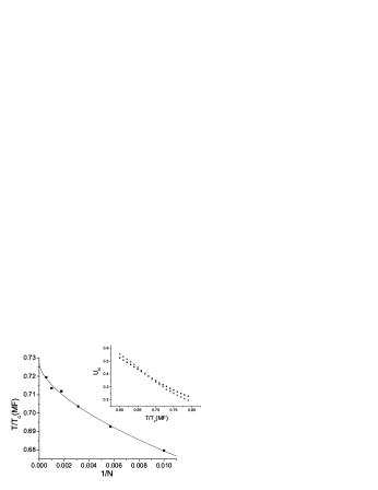
Figure 8: Finite-size estimate of the critical temperature (divided by the mean field estimate $JQ/k_{B}$) as a function of $1/N$ obtained using the intersections of the cumulants. An example of such an intersection is given in the second plot. The average connectivity is $Q=4$.

From the Binder cumulant, we can estimate the exponent $\alpha$. Indeed, the derivative of the cumulant $U^{\prime}_{N}=dU_{N}/dT$ at $T_{c}(N)$ scales as

$$\frac{U^{\prime}_{N}(T_{c})}{U^{\prime}_{N^{\prime}}(T_{c})}=\left(\frac{N}{N^{\prime}}\right)^{\frac{1}{2-\alpha}}$$ (58)

The derivative can be obtained from the polynomial fit used to determine $T_{c}(N)$. The values that we obtain are consistent with the assumption that $\alpha=0$.

Next, we calculated the magnetisation at $T_{c}(N)$ as a function of $N$. This allows us to estimate the exponent $\beta/(2-\alpha)$ as $\simeq 0.25$. In Fig. 9 (left side) we show our numerical results for $Q=10$. This result is consistent with the mean field values $\beta=1/2$ and $\alpha=0$. As a further test, we plotted the squared magnetisation as a function of $T$. Below $T_{c}$, we expect this to be a linear function and from a fit to this form we can get a second estimate of $T_{c}$ (see Fig. 9, right side). The values that we find in this way are in agreement with those coming from the cumulants, although the precision is less good.

Figure 9: $N$-dependence of the magnetisation of the SAN at $T_{c}(N)$ ($Q=10$). The slope is $-0.25\pm 0.01$. The right side shows the magnetization squared as a function of temperature for a network of 3200 nodes, averaged over 400 samples.

We also computed the finite-lattice susceptibility $\chi^{\prime}$, introduced by Binder 18

$$\chi^{\prime}\propto\langle M^{2}\rangle-\langle|M|\rangle^{2}$$ (59)

By taking the modulus of the magnetisation, one tries to minimise finite-size effects. Besides giving information about $T_{c}$, which is in agreement with the results coming from the cumulants and the magnetisation, the susceptibility provides information on the critical exponent $\gamma_{s}$. At $T_{c}$, one expects $\chi^{\prime}\propto N^{\gamma_{s}/(2-\alpha)}$. We calculated $\chi^{\prime}$ as a function of $N$ at a temperature close to $T_{c}$. We find that $\gamma_{s}/(2-\alpha)$ is close to $0.47\pm 0.03$, which is consistent with $\gamma_{s}=1$ using the earlier estimate of $\alpha$.

The plots for the specific heat as a function of temperature (Fig. 10, left side) look similar to those obtained from the cavity method. The specific heat does not diverge with size but saturates, which implies $\alpha\simeq 0$. However, the plots do not show the usual, mean field jump at $T_{c}$, but are in agreement with the presence of logarithmic corrections. The maximum in the specific heat below $T_{c}$ that was found within the cavity approach (Fig. 3) is also clearly visible in the data. When we change the value of $\mu$ from $1/2$ to $1$ we do find results consistent with the usual mean field behaviour, i.e. with a jump at $T_{c}$ (see Fig. 10, right side and compare with Fig. 4). Indeed $\mu=1$ corresponds to $\gamma^{\prime}\to\infty$, which corresponds to a network with a narrow degree distribution.

Figure 10: The specific heat as a function of temperature for a network of 5600 nodes (SAN model , left) and for the modified model with $\mu=1$ (right). Averages were taken over 400 samples. The average connectivity is $Q=10$.

We also performed a completely similar investigation of the network with $\mu=1/3$ and $Q=10$. In Fig. 11, we show log-log plots of the magnetisation (left) and the susceptibility (right) as a function of $N$ at the numerically determined value of $T_{c}$. From these data we obtain $\beta/(2-\alpha)=0.358\pm 0.001$ and $\gamma_{s}/(2-\alpha)=0.282\pm 0.002$. These results are consistent with the predictions coming from (12): $\beta/(2-\alpha)=1/3$ and $\gamma_{s}/(2-\alpha)=1/3$. The remaining discrepancy is probably due to errors in the determination of $T_{c}$. We also obtained data for the specific heat, but they do not allow a precise determination of $\alpha$. From (12), the prediction $\alpha=-1$ follows. This implies that the specific heat decreases linearly to its high-temperature background value. The data shown in Fig. 12 are consistent with this expectation.

Figure 11: Log-log plot of the magnetisation (left) and the susceptibility (right) versus $N$ at $T_{c}$ for the case $\mu=1/3,Q=10$.

Figure 12: The specific heat as a function of temperature for a network of 1000 nodes ($\mu=1/3$). The average connectivity is $Q=10$. Notice the linear regime for $8<k_{B}T/J<10.2$

From the simple mean field theory of section 2, it follows that the local order parameter $m_{i}\propto k_{i}^{1-\mu}$. We also used this relation in our derivation of the BP approximation. In order to get further confirmation for this type of scaling, we checked it numerically. Our results are shown in Fig. 13, for the cases $\mu=0,\ 0.5$ and $1$ on a BA-network. For high values of the degree, the statistics is not very good, but for smaller $k_{i}$-values the scaling (14) seems to be well satisfied.

Figure 13: The magnetization of individual spins as a function of degree for a network of 1000 nodes and different values of $\mu$. The averages are made over 1000 networks. The values of $\mu$ and the predicted $k$-dependence, respectively, is: $\mu=0$ - linear; $\mu=0.5$ - square root; $\mu=1$ - constant. The temperature is slightly below the respective critical temperatures.

We finally remark that for the SAN with $Q=2$, the Monte Carlo simulations indicate a zero critical temperature. Indeed, for this value of $Q$, the BA network has the structure of a tree and therefore it cannot support order. This is in contrast with the results coming from the replica approach. However, in that approach loops are not excluded and the network can be a collection of disconnected clusters, the largest of which determines the non-zero $T_{c}$ in the large-$N$ limit. To test this, we generated a set of random (uncorrelated) networks with $Q=2$ and $\gamma=3$ by ascribing to each vertex a degree taken from the distribution $P(k)$. The links going out of the vertices are then randomly paired to create a network. The resulting network is indeed found to consist of disconnected parts. In Fig. 14 we show Monte Carlo results for the Binder cumulant as a function of temperature for two networks ($N=2000$ and $N=4000$) generated in this way. We took $\mu=1/2$. Clearly there is an intersection from which we obtain the finite-size estimate for the critical temperature. After extrapolation ($N\to\infty$) we obtain from these kind of data $k_{B}T_{c}/J=0.92648$. For comparison, the BP prediction for $kT_{c}/J$ is $0.952$ and the replica method gives $0.946$ (Table 1).

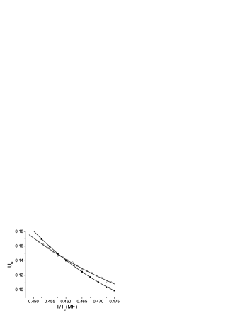
Figure 14: Binder cumulants as a function of temperature for a network with $\gamma=3,Q=2$ and $\mu=1/2$. The figure shows a clear intersection of the cumulants for $N=2000$ (circles) and $N=4000$ (squares) indicating the presence of a critical point at finite temperature. The averages were done over 6000 and 5000 realizations of the networks, respectively. The fit with a third degree polynomial is also shown in the figure.

VI Nonequilibrium models

In this section, we show that the basic result of this paper, (12), is also true for a nonequilibrium model. In particular, we will investigate the contact process 23 on a network. This process is a well known model originally introduced to describe the spreading of a disease in a population. Later, it was found to be related to directed percolation 26 and became the prototype model used in the study of absorbing state phase transitions 25 . Recently the contact process has also been applied in metapopulation ecology 24 , but in this paper we will use the epidemiological language.

On a network we define the contact process as follows. Each vertex $i$ can be in two states that we denote as ill ($n_{i}=1$) and healthy ($n_{i}=0$). The dynamics of the model is given by a continuous time Markov process 81 . An ill site can cure with a rate 1 (this fixes the time scale). A healthy site becomes ill with a rate that equals $\lambda$ times the number of ill neighbours, where on a network two vertices are called neighbours’ if they are linked.

This model has an absorbing state: if all sites are healthy, they will stay healthy forever. For an infinite system, there is a phase transition at some $\lambda_{c}$. If $\lambda\leq\lambda_{c}$, the system will evolve to the absorbing state. For $\lambda>\lambda_{c}$, there will always be a finite density of ill’ sites. This density is the order parameter of the model and it goes to zero if one approaches $\lambda_{c}$ from above. Vespignani and coworkers 19 ; 20 showed that on a scale-free network for $2<\gamma\leq 3$, $\lambda_{c}=0$ and the exponents are $\gamma$-dependent. For $3<\gamma\leq 4$, $\lambda_{c}>0$ and the critical exponents are again $\gamma$-dependent. Finally, for $\gamma>4$, $\lambda_{c}>0$ and critical exponents assume the mean-field values for the contact process on a regular lattice. This scenario is reminiscent of that for the opinion formation model.

We next generalise the contact process by taking the infection rate as

$$\lambda_{ij}=\lambda Q^{2\mu}(k_{i}k_{j})^{-\mu}$$ (60)

Using standard techniques from the theory of stochastic processes 81 , one can show that $\rho_{i}=\langle n_{i}\rangle$ (where $\langle.\rangle$ in this paragraph denotes the average over histories of the stochastic process) obeys the exact equation

$$\frac{d\rho_{i}}{dt}=-\rho_{i}+\sum_{l}\lambda_{il}\langle(1-n_{i})n_{l}\rangle$$ (61)

The sum runs over the neighbours of $i$. We now make two approximations similar to those performed in section 2. The first one, the dynamical mean field approximation, puts $\langle(1-n_{i})n_{l}\rangle\approx\langle(1-n_{i})\rangle\langle n_{l}\rangle=(1-\rho_{i})\rho_{l}$. Next, again following Bianconi 7 , we replace the sum over the neighbours by a sum over all the nodes, and take for $\lambda_{ij}$ its average over all realisations of the network with a given set of degrees. Then (61) becomes

$$\frac{d\rho_{i}}{dt}=-\rho_{i}+(1-\rho_{i})\sum_{j=1}^{N}[\lambda_{ij}]\rho_{j}$$ (62)

Now (see section 2) $[\lambda_{ij}]=\lambda_{ij}p_{ij}$ with $p_{ij}=k_{i}k_{j}/(QN)$, the probability that nodes $i$ and $j$ are connected. This gives

$$\frac{d\rho_{i}}{dt}=-\rho_{i}+(1-\rho_{i})\frac{\lambda Q^{2\mu-1}}{N}k_{i}^{1-\mu}\sum_{j=1}^{N}k_{j}^{1-\mu}\rho_{j}$$ (63)

We introduce $\Theta$

$$\Theta=\frac{Q^{\mu-1}}{N}\sum_{j=1}^{N}k_{j}^{1-\mu}\rho_{j}$$ (64)

From here on, we will assume that $\rho_{i}$ depends only on the degree of $i$. We can then write for a large network

$$\Theta=Q^{\mu-1}\sum_{k}P(k)k^{1-\mu}\tilde{\rho}_{k}$$ (65)

where $\tilde{\rho}_{k}$ is the density of sites that are ill and have degree $k$.

Using (64) and this assumption, (63) becomes

$$\frac{d\tilde{\rho}_{k}}{dt}=-\tilde{\rho}_{k}+\lambda(1-\tilde{\rho}_{k})Q^{u}k^{1-\mu}\Theta$$ (66)

We are interested in the static properties, i.e. the properties of the model in the long time limit. Then, from (66) we get

$$\tilde{\rho}_{k}=\frac{\lambda Q^{\mu}k^{1-\mu}\Theta}{1+\lambda Q^{\mu}k^{1-\mu}\Theta}$$ (67)

Using (65), we find a self-consistency equation for $\Theta$

$$\Theta=\lambda Q^{2\mu-1}\sum_{k}P(k)\frac{k^{2-2\mu}\Theta}{1+\lambda Q^{\mu}k^{1-\mu}\Theta}$$ (68)

We can now in principle analyse this equation.

But as was the case for the opinion formation model, it is easier to transform away the $\mu$-dependence. This is most easily done by rewriting (68) as an integral

$$\Theta=A\lambda Q^{2\mu-1}\int_{m}^{\infty}k^{-\gamma}\frac{k^{2-2\mu}\Theta}{1+\lambda Q^{\mu}k^{1-\mu}\Theta}dk$$ (69)

where $A$ is a normalisation constant and where the power-law form for $P(k)$ is inserted. If we change variables to $k^{\prime}=Q^{\mu}k^{1-\mu}$, (10) becomes (if $\mu\leq 1$)

$$\Theta=A^{\prime}\int_{m^{\prime}}^{\infty}(k^{\prime})^{\frac{1-\gamma}{1-\mu}}\frac{k^{\prime}\Theta}{1+\lambda k^{\prime}\Theta}dk^{\prime}$$ (70)

where $A^{\prime}$ is another constant and $m^{\prime}=m^{1-\mu}Q^{\mu}$.

This is precisely the form (69) assumes for $\mu^{\prime}=0$ provided we shift $\gamma$ to $\gamma^{\prime}$ given by

$$\gamma^{\prime}=\frac{\gamma-\mu}{1-\mu}$$ (71)

Thus, the same relation holds as for the static Ising case 27 . But notice that now, taking $\mu=1/2$ and a Barabasi-Albert network (i.e. the epidemiological version of the SAN), leading to $\gamma^{\prime}=5$, we are in a situation where mean-field theory should hold without logarithmic corrections.

The relation (12) thus appears to be quite general and one may wonder whether there are any exceptions to it. We first discuss a recently proposed realization of the Bak-Tang-Wiesenfeld sandpile model on scale-free networks 22 . In this model an avalanche can be generated through the following dynamical rules: 1) at each time step, a grain is added at a randomly chosen network node $i$; 2) if the height $h_{i}$ at node $i$ exceeds a given threshold $z_{i}$, it becomes unstable and an integer number of grains, $n[z_{i}]$, at the node topple, with $n[z_{i}]-1<z_{i}\leq n[z_{i}]$, to randomly chosen $n[z_{i}]$ nodes among $k_{i}$ adjacent ones; 3) whenever adjacent nodes become unstable toppling takes place also there, on all unstable nodes in parallel, and the avalanche continues until there are no unstable nodes left. In the proposed version of the model 22 , a parameter $\eta$ is introduced and the threshold $z_{i}$ of node $i$ is taken to be

$$z_{i}=k_{i}^{1-\eta}$$ (72)

Note that for $\eta=0$ the model features a simple degree-dependent threshold, and in the extended model $k$ is replaced by $k^{1-\eta}$. Note that this is reminiscent of the transformation $k\rightarrow k^{1-\mu}$ which we discussed in other contexts in this paper.

A key quantity in the description of the avalanche dynamics by mapping each avalanche to a tree, is the branching probability $P_{b}(n)$ that a node, which receives a grain from a neighbour, generates $n$ branches. This probability consists of two factors 22 . If branching occurs for a given node $i$, $n[z_{i}]$ branches are generated. Therefore, the first factor, $P_{1}(n)$, is the probability that $n$ coincides with $n[z_{i}]$ for a node $i$ already connected to the tree. The second factor is the probability that the height $h_{i}$ takes the value $n-1$ at the moment that node $i$ receives a grain from a neighbour. This probability, $P_{2}(n)$, is not important for us here, but in the case of independent random heights ${0,1,...,n-1}$ in the inactive state of the sandpile, it equals $1/n$. If we would adopt a continuum approximation, treating $n$ as a real number, and approximate $n[z_{i}]$ by $z_{i}$, we would arrive at the result

$$P_{b}(n)=(n^{1/(1-\eta)}P(n^{1/(1-\eta)})/Q)P_{2}(n),$$ (73)

where the first factor, $P_{1}(n)=kP(k)/Q$, is the probability that the first neighbour of a node has degree $k$, with in our case $k=n^{1/(1-\eta)}$. This probability differs from $P(k)$ in that it presupposes that the generating node is already connected to the tree.

If we compare this $P_{b}(n)$ with its counterpart for the model with $\eta=0$, we easily observe that the extended model is equivalent to the basic model with $\eta^{\prime}=0$, provided the topological exponent is transformed according to

$$\gamma^{\prime}=\frac{\gamma-\eta}{1-\eta}$$ (74)

This is in agreement with our general exponent relation, but, as we shall show now, and as Goh et al. already found 22 this result is incorrect.

The correct exponent relation is found when taking into account properly that $n$ is always an integer, and that all thresholds in the interval $n-1<z_{i}\leq n$ contribute to the probability of generating $n$ branches. $P_{1}(n)$ thus consists of a sum, or, for simplicity and without loss of relevant precision, an integral, so that

$$P_{b}(n)=(\int_{(n-1)^{1/(1-\eta)}}^{n^{1/(1-\eta)}}kP(k)dk/Q)P_{2}(n),$$ (75)

from which follows the correct relation

$$\gamma^{\prime}=\frac{\gamma-2\eta}{1-\eta},$$ (76)

which was already obtained by Goh et al 22 . We conclude that an exception to our general exponent relation arises here due to the discrete (integer) character of the toppling process. Indeed, the general relation is recovered in a (rough) continuum approximation of the problem.

A second exception to our general exponent relation is provided by the study of Dezsö and Barabási 22bis of disease spreading on a scale-free network. The model they consider starts from the usual contact process, for which it is known that the epidemic threshold $\lambda_{c}$ vanishes for $\gamma\leq 3$. This is similar to the divergence of the critical temperature for an Ising model with constant interactions on a scale-free network. We have seen that topology-dependent interactions are a way to get around this and we have discussed this in detail also for the contact process.

However, Dezsö and Barabási provide an alternative means of rendering the epidemic threshold finite and thus offering new avenues for controlling diseases (e.g., eradicating viruses). Their strategy consists of curing the hubs with a probability that scales with the degree $k$ of a node as $k^{\alpha}$. Note that $\alpha=0$ corresponds to the usual model in which all nodes are cured with the same probability.

As a result Eq. (69) takes the modified form 22bis

$$\Theta=A\lambda Q^{-1}\int_{m}^{\infty}k^{-\gamma}\frac{k^{2}\Theta}{k^{\alpha}+\lambda k\Theta}dk,$$ (77)

from which we can derive the following exponent relation

$$\gamma^{\prime}=\frac{\gamma-2\alpha}{1-\alpha},$$ (78)

with $\gamma^{\prime}$ the effective topological exponent for an equivalent model with degree-independent curing rate ($\alpha^{\prime}=0$). Curiously, this new relation is akin to that of the previous exception (sandpile model), but this coincidence has to our insight no significance.

VII Discussion

In this paper, we investigated the critical properties of an Ising model and a contact process with topology-dependent interactions on scale-free networks. The interaction strength between two spins, or the infection rate between two individuals, was assumed to be proportional to $(k_{i}k_{j})^{-\mu}$. We have developed mean-field theories for these models from which our main result follows: the critical behaviour can always be related to that of the corresponding model with homogeneous couplings ($\mu^{\prime}=0$) on a network with a modified degree distribution $\gamma^{\prime}$, where $\gamma^{\prime}$ is given by equation (12). Due to the small-world property of scale-free networks, mean field theory is generally believed to be exact. This expectation is found to be true also in the present case. We performed extensive numerical calculations for the Ising model on a BA-network, focusing on the cases $\mu=1/2$ (the SAN, which was the original motivation for the present work) and $\mu=1/3$. We used two techniques: numerically exact’ studies with the cavity approach, and Monte Carlo simulations. The first approach assumes the absence of loops in the network, which is a good approximation for a BA-network. The Monte Carlo calculations approximate the true thermal average by an average over a finite set of well chosen spin configurations. Within their numerical accuracy, both approaches give the same results. More importantly, they provide strong evidence that the exponent relation (12) is correct.

For static network ensembles it is possible to obtain an exact equation for the location of the critical temperature from the replica approach, see equations (55) and (56). A simpler equation for this quantity, (32), can be derived from the Bethe-Peierls approximation. From the numerical values listed in table 1, it can be seen that this simple aproach gives results that are accurate to better than one percent. From the table one also observes that the differences in the critical temperature as obtained from the different approaches are very small for $Q\geq 4$.

Besides the contact process, the behaviour of several other (non) equilibrium models have been studied on scale-free networks. In particular, we mention here diffusion-annihilation 21 and the Bak-Sneppen model 255 . In both cases, the critical behaviour shows a $\gamma$-dependence that is reminiscent of that of the Ising model and the contact process. It remains to be investigated whether appropriately extended versions of these models obey the relation (12) or whether they follow modified transformation laws as we found to be the case for the sandpile model of ref. 43 or the modified contact process of ref. 44.

References

- (1) R. Albert and A.-L. Barabási, Rev. Mod. Phys. 74, 47 (2002).
- (2) S.N. Dorogovtsev and J.F.F. Mendes, Evolution of networks: from biological nets to the internet and WWW, Oxford University Press (2003).
- (3) B. Bollobás, Random Graphs, Cambridge University Press (2001).
- (4) D.J. Watts and S.H. Strogatz (1998), Nature 393 440 (1998).
- (5) S. Maslov, K. Sneppen and U. Alon in Handbook of graphs and networks edited by S. Bornholdt and H.G. Schuster, Wiley (2003), p. 168.
- (6) R. Pastor-Satorras and A. Vespignani, Evolution and structure of the internet: a statistical physics approach, Cambridge University Press (2004).
- (7) H. Jeong, B. Tombor, R. Albert, Z.N. Oltvai and A.-L. Barabási, Nature 407, 651 (2000).
- (8) R.V. Solé and A. Munteanu, Europhys. Lett. 68, 170 (2004).
- (9) L.A.N. Amaral and J.M. Ottino, Eur. Phys. J. B 38, 147 (2004).
- (10) A.-L. Barabási and R. Albert, Science 286, 509 (1999).
- (11) S. Galam, Y. Gefen, and Y. Shapir, J. Math. Sociology 9, 1 (1982); K. Sznajd-Weron and J. Sznajd, Int. J. Mod. Phys. C 11, 1157 (2000).
- (12) A. Aleksiejuk, J.A. Holyst, and D. Stauffer, Physica A 310, 260 (2002).
- (13) S.N. Dorogovtsev, A.V. Goltsev, and J.F.F. Mendes, Phys. Rev. E 66, 016104 (2002).
- (14) M. Leone, A. Vázquez, A. Vespignani, and R. Zecchina, Eur. Phys. J. B 28, 191 (2002).
- (15) A.V. Goltsev, S.N. Dorogovtsev, and J.F.F. Mendes, Phys. Rev. E 67, 026123 (2003).
- (16) F. Iglói and L. Turban, Phys. Rev. E 66, 036140 (2002).
- (17) J.O. Indekeu, Physica A 333, 461 (2004).
- (18) C.V. Giuraniuc, J.P.L. Hatchett, J.O. Indekeu, M. Leone, I. Pérez Castillo, B. Van Schaeybroeck and C. Vanderzande, Phys. Rev. Lett. 95, 098701 (2005).
- (19) G. Bianconi, Phys. Lett. A 303, 166 (2002).
- (20) J.S. Yedidia in Advanced Mean field methods: theory and practice, edited by M. Opper and D. Saad, MIT press (2001).
- (21) M. Mézard, G. Parisi and M.A. Virasoro, Spin glass theory and beyond, World Scientific (1987).
- (22) M. Mézard and G. Parisi, Eur. Phys. J. B 20, 217 (2001)
- (23) M. Mézard and G. Parisi, J. Stat. Phys. 111, 1 (2003).
- (24) M. Newman, Phys. Rev. Lett. 89, 208701 (2002).
- (25) A. Vázquez and M. Weight, Phys. Rev. E 67, 027101 (2003).
- (26) G. Bianconi and A. Capocci, Phys. Rev. Lett. 90, 078701 (2003).
- (27) H.D. Rozenfeld, J.E. Kirk, E.M. Bollt and D. ben-Avraham, J. Phys. A 38, 4589 (2005).
- (28) R.J. Baxter, Exactly solved models in statistical mechanics, Academic Press (1982).
- (29) R. Kikuchi, Phys. Rev. 81, 988 (1951).
- (30) K. Y. Wong and D. Sherrington, J. Phys. A 21, L459 (1988)
- (31) K. Binder, Z. Phys. B 43, 119 (1981).
- (32) K. Binder, Phys. Rev. Lett. 47, 693 (1981).
- (33) A.M. Ferrenberg and D.P.Landau, Phys. Rev. B 43, 5081 (1991).
- (34) K. Binder in The Monte Carlo method in the Physical Sciences edited by J.E. Gubernatis AIP Conference Proceedings, Vol 690, Springer Verlag (2003).
- (35) T. E. Harris, Ann. Prob. 2, 969 (1974).
- (36) P. Grassberger and A. de la Torre, Ann. Phys. (NY) 122, 373 (1979).
- (37) R. Dickman in Nonequilibrium statistical mechanics in one dimension edited by V. Privman , Cambridge University Press (1997).
- (38) V. Vuorinen, M. Peltomäki, M. Rost and M.J. Alava, Eur. Phys. J. B 38, 261 (2004).
- (39) N.G. Van Kampen, Stochastic processes in physics and chemistry, North-Holland (1992).
- (40) R. Pastor-Satorras and A. Vespignani, Phys. Rev. E 63, 066117 (2001).
- (41) R. Pastor-Satorras and A. Vespignani in Handbook of graphs and networks edited by S. Bornholdt and H.G. Schuster, Wiley (2003).
- (42) This extension of the exponent relation to nonequilibrium models was independently obtained in M. Karsai, R. Juhász and F. Iglói, Phys. Rev. E 73, 036116 (2006)
- (43) K.-I. Goh, D.-S. Lee, B. Kahng and D. Kim, Physica A 346, 93 (2005).
- (44) Z. Deszö and A.-L. Barabási, Phys. Rev. E 65, 055103(R) (2002).
- (45) M. Catanzaro, M. Boguña and R. Pastor-Satorras, Phys. Rev. E 71, 056104 (2005).
- (46) S. Lee and Y. Kim, Phys. Rev. E 71, 057102 (2005).