Nonadiabatic production of spinor condensates with a QUIC trap

Abstract

Motivated by the recent experimental observation of multi-component spinor condensates via a time-dependent quadrupole-Ioffe-configuration trap (QUIC trap), we provide a general framework for the investigation of nonadiabatic Landau-Zener dynamics of a hyperfine spin, e.g., from an atomic magnetic dipole moment coupled to a weak time-dependent magnetic (B-) field. The spin flipped population distribution, or the so-called Majorona formula is expressed in terms of system parameters and experimental observables; thus, provides much needed insight into the underlying mechanism for the production of spinor condensates due to nonadiabatic level crossings.

I Introduction

Magnetic traps play an important role in the study of atomic Bose-Einstein condensates (BEC) magnetictrap . In a typical static magnetic trap, individual atomic spin couples to the spatial dependent magnetic (B-) field because of Zeeman effect. When an atom moves in a region where the direction of the B-field changes slowly and the strength of the B-field is sufficiently strong, according to Born-Oppenheimer approximation bo1 ; bo2 , the atomic spin can follow the B-field adiabatically and remain in the same trapped eigen-state of the interaction Hamiltonian relative to the instantaneous direction of the magnetic field ${\vec{B}}({\vec{r}})$, where ${\vec{r}}$ is the center of mass position of the atom (or more precisely, that of the valence electron). In this case the atomic center of the mass experiences an effective spatially-varying potential that is equal to the Zeeman energy and proportional to the strength of the B-field.

For weak B-fields, when the atomic Zeeman energy is comparable to or less than the frequency of the directional variation of the B-field felt by the moving atom, adiabatic dynamics cannot be followed anymore. As a result, nonadiabatic (Majorona) transitions Majorona for the atomic spin may occur. Two potentially damaging effects can cause nonadiabatic transitions. The first happens when an atom enters a weak B-field region due to its translational motion in space. For instance, in a quadrupole trap, atoms in the weak field seeking state are accelerated towards the center of the trap where the B-field vanishes. Nonadiabatic transitions always occur in the vicinity of a zero B-field. To avoid this region of vanishing B-field or a spatial ”hole,” a number of methods have been developed to effectively plug it, e.g., with the use of a far-off-resonant optical potential as an “optical plug” opticalplug or the more famous time averaged orbiting potential (TOP) trap top . The second reason for nonadiabatic transitions is due to the explicit time dependence of the B-field. Obviously nonadiabatic transitions may occur if the B-field changes rapidly with time.

Recently, the atomic quantum gas group at Peking University (PKU) reported interesting observations of multi-component ⁸⁷Rb ($F=2$) spinor condensates via switching off the B-fields of an initially spin polarized single component condensate in a QUIC trap chenshuai . The group of Prof. Chandra Raman at Georgia Tech also discovered counter-intuitive meta-stability when condensates were loaded into an “unplugged” magnetic quadruple trap raman . We decided to present our theoretical studies in the hope that the theoretical framework for spinor nonadiabatic level crossing dynamics may be of interest to other groups in the field of atomic quantum gases. In this paper, we will focus on the Peking University experiment in a time-dependent QUIC trap hansch . The more involved situation of a condensate in a quadruple trap will be discussed elsewhere peng . According to the reported experiment chenshuai , the affected time-dependence for the B-field is relatively simple. After a single component condensate was created in a QUIC trap, the various B-field generating currents were switched off in appropriately chosen orders. Whenever near-zero level-crossing occurs, multi-component spinor condensates are observed.

This paper summarizes our treatment of level crossing dynamics for an atomic spin inside an external B-field. The theory is developed with respect to “the first scenario,” where the vanishing B-field is due to the different time constants of decay for the B-fields from the QUIC coil and the bias coil after being shut off as discussed in Sec. II. An alternative scenario where the B-field zero is due to different time constants of the decaying B-fields from the quadruple coil and the Ioffe coil will be discussed in Sec. III. Finally we conclude and provide a brief summary in Sec. IV.

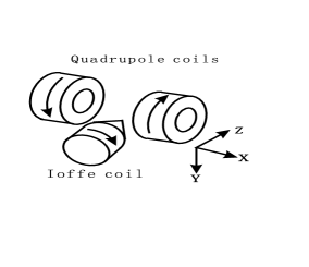
Figure 1: The QUIC trap geometry (excluding the bias coils). The arrows indicate directions of currents in the coils.

II The First Scenario

The magnetic trap used in their experiment chenshuai is made up from two separate coils, a QUIC coil and a bias coil. The QUIC coil consists of a quadruple trap coil and an Ioffe coil in series as in the original QUIC trap hansch . The compensating coils for the earth’s B-field are separate and always left on; thus will not be included explicitly in our model. Before switching off, the magnetic B-field ${\vec{B}}^{\rm Q}({\vec{r}})$ created by the QUIC coil has the familiar configuration of a Ioffe-Pritchard trap and can be expressed as chenshuai ; hansch

$${\vec{B}}^{\rm Q}({\vec{r}})=B^{\rm Q}_{\perp}({\vec{r}})\mathbf{e}_{\mathbf{\perp}}+B^{\rm Q}_{z}({\vec{r}})\mathbf{e}_{\mathbf{z}},$$ (1)

where the axial and radial QUIC B-field components are $B^{\rm Q}_{\perp}({\vec{r}})$ and $B^{\rm Q}_{z}({\vec{r}})$, respectively;

$$B^{\rm Q}_{z}({\vec{r}}) = B^{\rm Q}_{z}(0)+B^{\rm Q\prime\prime}_{z}z^{2},$$

$$B^{\rm Q}_{\perp}({\vec{r}}) = B^{\mathrm{Q\prime}}_{\perp}\sqrt{x^{2}+y^{2}},$$ (2)

with the unit vector $\mathbf{e}_{\mathbf{\perp}}$ defined as

$$\mathbf{e}_{\mathbf{\perp}}=\frac{(-x\mathbf{e}_{x}+y\mathbf{e}_{y})}{\sqrt{x^{2}+y^{2}}}.$$ (3)

$B^{\mathrm{Q\prime}}_{\perp}$ and $B^{\rm Q\prime\prime}_{z}$ denote the respective spatial derivatives for the B-fields. The right handed coordinate system as in Figure 1 is chosen such that $B^{\rm Q}_{z}(0)>0$ and $B^{\mathrm{Q\prime}}_{\perp}>0$.

The bias field ${\vec{B}}^{\rm A}$ is in the $z$ direction. It is created by the bias coils and approximately constant near the trap center chenshuai . Before switching off, it can be expressed as ${\vec{B}}^{\rm A}({\vec{r}})=-B^{\rm A}_{z}\mathbf{e}_{\mathbf{z}}$ satisfying $B^{\rm Q}_{z}(0)>B^{\rm A}_{z}>0$. If the bias field is switched off first and the two components of the QUIC field are simultaneously switched off after a time interval of $t_{\mathrm{int}}$, then at time $t$, the QUIC field becomes $e^{-t/\tau_{\rm Q}}{\vec{B}}^{\rm Q}({\vec{r}})$ and the bias field becomes $e^{-(t+t_{\mathrm{int}})/\tau_{\rm A}}{\vec{B}}^{\rm A}({\vec{r}})$, i.e., both the QUIC field and the bias field are assumed to decrease exponentially with decay time constants $\tau_{Q}$ and $\tau_{A}$, and the quadruple field and the Ioffe field are assumed to decay with the same time constant. Assuming $t=0$ as the instant for shutting off the QUIC field, the total time-dependent B-field then becomes

$${\vec{B}}({\vec{r}},t) = e^{-t/\tau_{Q}}B^{\rm Q}_{\perp}({\vec{r}})\mathbf{e}_{\mathbf{\perp}}$$ (4)

$$+e^{-t/\tau_{Q}}B^{\rm Q}_{z}({\vec{r}})\mathbf{e}_{\mathbf{z}}-e^{-(t+t_{\mathrm{int}})/\tau_{\rm A}}B^{\rm A}_{z}\mathbf{e}_{\mathbf{z}}.$$

$B^{\rm Q}_{\perp}({\vec{r}})$ is proportional to $(x^{2}+y^{2})^{1/2}$ near the trap center or the origin; therefore, we have $B^{\rm Q}_{z}({\vec{r}}),\ B^{\rm A}_{z}\gg B^{\rm Q}_{\perp}({\vec{r}})$ and $|B^{\rm Q}_{z}({\vec{r}})-B^{\rm A}_{z}|\gg B^{\rm Q}_{\perp}({\vec{r}})$. Before switching off the QUIC field, the $z$ component of ${\vec{B}}({\vec{r}},t)$ takes a positive value $B^{\rm Q}_{z}({\vec{r}})-B^{\rm A}_{z}$ much larger than the initial value of the transverse field $B^{\rm Q}_{\perp}({\vec{r}})$. At $t=0$, all atomic spins initially are polarized, thus are the eigen-state $|M_{F}=2\rangle$ of $F_{z},$ i.e., the $z$ component of the atomic hyperfine spin $\vec{F}$. If the QUIC field and the bias field are switched off simultaneously, i.e., $t_{\mathrm{int}}=0$ and $\tau_{Q}=\tau_{A}$, the direction of the total B-field ${\vec{B}}({\vec{r}},t)$ does not change with time although the strength of ${\vec{B}}({\vec{r}},t)$ decreases after the switching off process. Nonadiabatic transitions do not occur in this case and the initial single component condensate remains a single component one. If the QUIC field and the bias field decrease with different time constants $\tau_{\rm Q}\neq\tau_{\rm A}$, the direction of ${\vec{B}}({\vec{r}},t)$ changes with time and nonadiabatic level crossing arises.

In the calculations to follow, we will make a simple approximation that the atomic spatial position does not change during the switching-off process. This allows for an easy calculation of nonadiabatic transition probabilities between different atomic spin states at a fixed spatial position ${\vec{r}}$. This is well justified for the experiment of PKU, where level crossing occurs over a time window of $\sim 10^{2}(\mu{\mathrm{s}})$, during which an condensed atom moves a distance less than $0.1(\mu{\mathrm{m}})$, provided its kinetic energy is $\sim 10^{4}({\mathrm{Hz}})$.

As mentioned above, the $z$ component of the B-field initially takes a large positive value. After the switching-off, the bias field decreases much slower than the QUIC field chenshuai , i.e. we have $\tau_{\rm A}\gg\tau_{\rm Q}$. At certain instant $t_{0}$, the value of $e^{-t/\tau_{Q}}B^{\rm Q}_{z}$ equals $e^{-(t+t_{\mathrm{int}})/\tau_{\rm A}}B^{\rm A}_{z}$, which causes the $z$ component of the total B-field to become zero. As a result of this, transitions from the state $|M_{F}=2\rangle$ to other eigen-states of $F_{z}$ occur because of the finite transverse B-field $e^{-t/\tau_{Q}}B^{\rm Q}_{\perp}$ in the vicinity of $t_{0}$. After $t_{0}$, the $z$ component of the B-field becomes negative because $e^{-(t+t_{\mathrm{int}})/\tau_{\rm A}}/e^{-t/\tau_{Q}}\gg 1$ for a large enough $t$; the absolute value of the $z$ component of the B-field can become again much larger than the transverse components of ${\vec{B}}({\vec{r}},t)$ for $t\gg t_{0}$. Therefore, the probabilities for an atom in different eigen-states of $F_{z}$ can again take constant values in the long time limit.

To compute the nonadiabatic level crossing rates, we note that transitions mainly occur in the near zero B-field region, i.e., for weak B-field. Thus, we only need to consider the linear Zeeman coupling of an atomic hyperfine spin. Our model Hamiltonian takes the simple form

$$H=g_{F}\mu_{{\mathrm{B}}}{\vec{B}}({\vec{r}},t)\cdot\vec{F}.$$ (5)

Here $g_{F}$ is the Land$\acute{\rm e}$ $g$ factor and $\mathrm{\mu}_{\mathrm{B}}$ is the Bohr magneton. For ⁸⁷Rb atoms under consideration here, the spinor degree of freedom refers to the $F=2$ manifold with $g_{F}=1/2$. In their experiment chenshuai , the initial condition corresponds to

$$|\Psi(0)\rangle=|M_{F}=2\rangle.$$ (6)

At large $t\rightarrow+\infty$, the wave function can be expanded as

$$|\Psi(t\rightarrow+\infty)\rangle=\sum_{M_{F}=-2}^{2}C_{M_{F}}({\vec{r}})e^{-i\phi_{M_{F}}({\vec{r}},t)}|M_{F}\rangle,$$ (7)

in the complete basis of $F_{z}$ along the initial quantization axis. Our problem is to find the steady population distribution $P_{M_{F}}({\vec{r}})=|C_{M_{F}}({\vec{r}})|^{2}$ in the long time limit.

We will make use of the method of Hioe hioe to calculate the finial state probability distribution due to nonadiabatic level crossing of a high spin. Because of the rotational symmetry of our model system (5), it can be mapped onto a spin $1/2$ spinor with the same type of coupling, described by a Hamiltonian

$$H_{\sigma}=g_{F}\mu_{\mathrm{B}}{\vec{B}}(\vec{r},t)\cdot{\frac{\vec{\sigma}}{2}},$$ (8)

where $\vec{\sigma}$ is the familiar spin $1/2$ Pauli matrix vector. The initial condition for the spin $1/2$ state is

$$|\varphi(0)\rangle=[1,0]^{T},$$ (9)

and the finial state can be denoted as

$$|\varphi(t\rightarrow+\infty)\rangle=[\alpha({\vec{r}})e^{i\phi_{\alpha}({\vec{r}},t)},\beta({\vec{r}})e^{i\phi_{\beta}({\vec{r}},t)}]^{T}.$$ (10)

Upon solving this two state problem, $P_{M_{F}}({\vec{r}})$ can be found easily according to the rotation group representation elements as in Hioe hioe . Apart from a globe phase factor, the evolution operator corresponding to the Hamiltonian (5) can be expressed as $D^{(2)}=\exp[-i\hat{n}\cdot\vec{F}\theta]$; while the one corresponding to the Hamiltonian (8) is $D^{(1/2)}=\exp[-i\hat{n}\cdot(\vec{\sigma}/2)\theta]$. The unit vector $\hat{n}$ and the angle $\theta$ are determined by $\vec{B}(\vec{r},t)$. Therefore, $D^{(1/2)}$ and $D^{(2)}$ are the representation matrixes (D matrixes) of the same rotation operation. The transition probabilities $P_{M_{F}}$ and $|\alpha(\vec{r})|^{2}$ can be rewritten as $P_{M_{F}}=|D^{(2)}_{M_{F},2}|^{2}$ and $|\alpha(\vec{r})|^{2}=|D^{(1/2)}_{1/2,1/2}|^{2}$. According to the representation theory of ${\rm SO}(3)$ group winger , $|D^{(2)}_{1/2,1/2}|$ and $|D^{(2)}_{M_{F},2}|$ are functions of $\sin[\beta/2]$ and $\cos[\beta/2]$ with $\beta$ one of the three Euler angles of the rotation. Although we do not know the values of $\hat{n},\theta$, and $\beta$, we can express the transition probability $P_{M_{F}}$ in terms of $A({\vec{r}})=|\alpha({\vec{r}})|^{2}$; as,

$$P_{2}({\vec{r}}) = A({\vec{r}})^{4},$$

$$P_{1}({\vec{r}}) = 4A({\vec{r}})^{3}[1-A({\vec{r}})],$$

$$P_{0}({\vec{r}}) = 6A({\vec{r}})^{2}[1-A({\vec{r}})]^{2},$$ (11)

$$P_{-1}({\vec{r}}) = 4A({\vec{r}})[1-A({\vec{r}})]^{3},$$

$$P_{-2}({\vec{r}}) = [1-A({\vec{r}})]^{4}.$$

The two state problem can be solved accurately with the Landau-Zener formula lz . To this end, we reexpress the Hamiltonian (8) as

$$H_{\sigma}[t]=q[t]h_{\sigma}[t],$$ (12)

with the ”normalized” Hamiltonian

$$h_{\sigma}[t]=g_{\perp}\sigma_{\perp}+\left(g^{\rm Q}_{z}-e^{-\xi t}g^{\rm A}_{z}\right)\sigma_{z},$$ (13)

and the parameters

$$g_{\perp} = \frac{1}{2}g_{F}\mu_{\mathrm{B}}B^{\rm Q}_{\perp}({\vec{r}}),$$

$$g^{\rm Q}_{z} = \frac{1}{2}g_{F}\mu_{\mathrm{B}}B^{\rm Q}_{z}({\vec{r}}),$$

$$g^{\rm A}_{z} = \frac{1}{2}g_{F}\mu_{\mathrm{B}}e^{-t_{{\mathrm{int}}}/\tau_{{\mathrm{A}}}}B^{\rm A}_{z}({\vec{r}}),$$

$$\xi = (\tau_{\rm A}-\tau_{\rm Q})/{\tau}{{}_{\rm A}}{\tau}{{}_{\rm Q}}.$$ (14)

We define a new time variable

$$s=-\tau_{\rm Q}e^{-t/\tau_{Q}};$$ (15)

then, the time-dependent Schrödinger equation

$$i\partial_{t}|\varphi[t]\rangle=H_{\sigma}[t]|\varphi[t]\rangle,$$ (16)

becomes

$$i\partial_{s}|\varphi(s)\rangle=h(s)|\varphi(s)\rangle,$$ (17)

with $|\varphi(s)\rangle=|\varphi[t(s)]\rangle$ and $h(s)=h[t(s)]$. Consequently, the time interval of the dynamics $t\in[0,\infty]$ is mapped into $s\in[-\tau_{\rm Q},0].$

As stated above, the $z$ component of ${\vec{B}}({\vec{r}},t)$ takes large positive and negative values, respectively, at $t=0$ and $t=\infty$. Therefore, at $s=-\tau_{\rm Q}$ and $s=0$, the condition

$$\left|g^{\rm Q}_{z}-e^{-\xi t(s)}g^{\rm A}_{z}\right|\gg g_{\perp},$$ (18)

is satisfied while $g^{\rm Q}_{z}-e^{-\xi t(s)}g^{\rm A}_{z}$ takes positive and negative values, respectively. In the Landau-Zener approximation, a linear approximation is always assumed for the different energy levels. We find the value $s_{0}$ at the crossing point $t_{0}$ is given by

$$s_{0}=-\tau_{\rm Q}q(t_{0})=-\tau_{\rm Q}\left(\frac{g^{\rm A}_{z}}{g^{\rm Q}_{z}}\right)^{\frac{1}{\xi\tau_{\rm Q}}}.$$ (19)

At $s=s_{0}$ when the longitudinal B-field vanishes

$$\left(g^{\rm Q}_{z}-e^{-\xi t(s_{0})}g^{\rm A}_{z}\right)=0,$$ (20)

a linear approximation to the energy levels simply leads to

$$\left(g^{\rm Q}_{z}-e^{-\xi t(s)}g^{\mathrm{A}}_{z}\right)\approx v(s-s_{0}),$$ (21)

with

$$v = -g^{\rm A}_{z}\tau_{\rm Q}(\xi\tau_{\rm Q})\left(\frac{g^{\rm A}_{z}}{g^{\rm Q}_{z}}\right)^{-1-\frac{1}{\xi\tau_{\rm Q}}}.$$

Using the Landau-Zener formula, we immediately find

$$A({\vec{r}})=\exp\left(-\pi\frac{|g_{\perp}|^{2}}{|v|}\right).$$ (22)

For $\tau_{\rm A}\gg\tau_{\rm Q}$, we find $\xi\tau_{\mathrm{Q}}\approx 1$, which then leads to

$$A({\vec{r}},t_{\mathrm{int}}) \simeq \exp\left(-\pi\frac{|g_{\perp}|^{2}g^{\rm A}_{z}\tau_{\rm Q}}{g_{\rm Q}}\right)$$ (23)

$$= \exp\left(-\pi g_{F}\mu_{\mathrm{B}}B^{\rm A}_{z}({\vec{r}})\tau_{\rm Q}\frac{B^{\rm Q2}_{\perp}\left({\vec{r}}\right)}{2B^{\rm Q2}_{z}\left({\vec{r}}\right)}e^{-\frac{t_{\mathrm{int}}}{\tau_{\rm A}}}\right).\hskip 24.0pt$$

Obviously for a large enough time interval $t_{\mathrm{int}}$ such that $e^{-t_{\mathrm{int}}/\tau_{\rm A}}\ll 1$, we have $A({\vec{r}},t_{\mathrm{int}})\approx 1$ and $P_{2}({\vec{r}})\approx 1$. A single component condensate remains a single component one. In fact, if $e^{-t_{\mathrm{int}}/\tau_{\rm A}}\ll 1$, the bias field has already decreased to zero when the QUIC field is switched off. Thus, during the switching-off of the QUIC field, the direction of the B-field does not change and nonadiabatic transitions cannot occur.

In the experiment of PKU, chenshuai , the various trap parameters take the following values: $B^{\rm Q}_{z}(0)=9$ (Gauss), $B^{\rm A}_{z}=7.45$ (Gauss), $B^{\rm Q\prime\prime}_{z}=4.9\times 10^{2}$ (Gauss-cm^-2), $B^{\mathrm{Q}\prime}_{\perp}=3.0\times 10^{2}$ (Gauss-cm^-1), $\tau_{\rm Q}=40$ (${\mu}$s), $\tau_{\rm A}=3$ (ms). Before switching-off, the center of the QUIC trap is at ${\vec{r}}_{0}=(0,5\mathrm{\mu m},0)$. Substituting the above coefficient $A({\vec{r}})$ of Eq. (23) into Eq. (11), we arrive at a simple estimate for the population distribution $P_{M_{F}}({\vec{r}}_{0})$. More precisely, we can estimate the population distribution with the following,

$$N_{M_{F}}=\int P_{M_{F}}({\vec{r}})\rho({\vec{r}})d{\vec{r}},$$ (24)

where $\rho({\vec{r}})$ is the density profile of the trapped gas cloud. Figure 2 shows the typical dependence of such result on the time interval $t_{\mathrm{int}}$. In the calculation of Figure 2, we set $\rho({\vec{r}})$ to be the atomic density distribution given by the Thomas-Fermi approximation corresponding to the initial values of the QUIC field and the bias field. Namely, the spatial motion of the atoms is omitted. This approximation is based on the fact that the decay time $(\rm{3ms})$ is shorter than the period ($\sim$4.5-7.5ms) of the trap potential and seems to be a bit crude. To obtain a more accurate estimation of the atomic population, variations of the atomic spatial distribution in the decay process of the bias field should be considered fully .

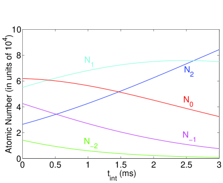
Figure 2: (Color online) A typical dependence of the population distributions on the time $t_{\mathrm{int}}$. The unit of the atomic number is $10^{-4}$.

The above result is based on the approximation that atoms do not move during the switching-off process. If atomic motion is included, more accurate population distribution can be calculated by solving the multiple-component Gross-Pitaevskii equation including the time-dependent B-field. A detailed comparison of these two approaches is given in Ref. peng . Overall, we find the approximate Landau-Zener solution discussed here holds well for the parameter regimes of the experiment chenshuai .

III An alternative scenario

The QUIC coil consists of a pair of quadruple coils and an Ioffe coil. The B-field ${\vec{B}}^{\mathrm{Q}}$ of the QUIC trap is the sum of the B-fields ${\vec{B}}^{\mathrm{qd}}$ from the quadruple coils and ${\vec{B}}^{\mathrm{If}}$ from the Ioffe coil. In the previous section, we simply assumed the B-fields generated by these two sets of coils decrease synchronously after shutting off electric currents . However, as was discovered in the experiment chenshuai , the magnetic fields ${\vec{B}}^{\mathrm{qd}}$ and ${\vec{B}}^{\mathrm{If}}$ do not always decay with the same time constant despite the fact that the two sets of coils forming the QUIC trap are in series. Assuming different time constants for the decay of ${\vec{B}}^{\mathrm{qd}}$ and ${\vec{B}}^{\mathrm{If}}$, the finial population distribution needs to be re-calculated.

Before the QUIC field is switched off, the components of the B-fields ${\vec{B}}^{\mathrm{qd}}$ and ${\vec{B}}^{\mathrm{If}}$ are functions of the atomic position, explicitly given by

$$\begin{array}[]{lll}B^{\mathrm{qd}}_{z}({\vec{r}})&=&B^{\mathrm{qd}\prime}(z-z_{0}),\\ B^{\mathrm{If}}_{z}({\vec{r}})&=&B^{\rm Q\prime\prime}_{z}z^{2}-B^{\mathrm{qd}\prime}(z-z_{0})+B^{\rm Q}_{z}(0),\\ B^{\mathrm{qd}}_{x}({\vec{r}})&=&-2B^{\mathrm{qd}\prime}x,\\ B^{\mathrm{If}}_{x}({\vec{r}})&=&(-B^{\mathrm{Q\prime}}_{\perp}+2B^{\mathrm{qd}\prime})x,\\ B^{\mathrm{qd}}_{y}({\vec{r}})&=&B^{\mathrm{qd}\prime}y,\\ B^{\mathrm{If}}_{y}({\vec{r}})&=&(B^{\mathrm{Q\prime}}_{\perp}-B^{\mathrm{qd}\prime})y,\end{array}$$

where $z_{0}$ is the distance between the center of the QUIC trap (in the absence of gravity) and the center of the quadruple trap.

In their experiment chenshuai , $B^{\mathrm{qd}\prime}$ is about $150$ (Gauss-cm^-1) and $z_{0}$ is $0.75$ (cm). Therefore, in the region near the center of the QUIC trap, we have $B^{\mathrm{qd}}_{z}=-107$ (Gauss). From $B^{\rm Q}_{z}(0)=9$ (Gauss), we find $B^{\mathrm{If}}_{z}=116$ (Gauss).

If ${\vec{B}}^{\mathrm{If}}$ and ${\vec{B}}^{\mathrm{qd}}$ decrease with different time constants $\tau_{\mathrm{If}}$ and $\tau_{\mathrm{qd}}$ after switching-off, the B-field from the quadruple coils becomes

$$(B^{\mathrm{qd}}_{z}\mathbf{e}_{z}+B^{\mathrm{qd}}_{y}\mathbf{e}_{y}+B^{\mathrm{qd}}_{x}\mathbf{e}_{x})e^{-t/\tau_{\mathrm{qd}}}$$ (25)

and the B-field created by the Ioffe coil becomes

$$(B^{\mathrm{If}}_{z}\mathbf{e}_{z}+B^{\mathrm{If}}_{y}\mathbf{e}_{y}+B^{\mathrm{If}}_{x}\mathbf{e}_{x})e^{-t/\tau_{\mathrm{If}}}.$$ (26)

In this section, we assume the time interval $t_{\mathrm{int}}$ between the switching-off of the B-fields ${\vec{B}}^{Q}$ and ${\vec{B}}^{A}$ is sufficiently long, i.e., when the QUIC field is switched off, the bias field has already decreased to zero. Since the B-fields $B^{\mathrm{qd}}_{z}$ and $B^{\mathrm{If}}_{z}$ have different signs, at a time $\tilde{t}_{0}$ the condition

$$B^{\mathrm{If}}_{z}e^{-\tilde{t}_{0}/\tau_{\mathrm{If}}}+B^{\mathrm{qd}}_{z}e^{-\tilde{t}_{0}/\tau_{\mathrm{qd}}}=0$$ (27)

can be satisfied and the $z$ component of the total B-field becomes zero. As before, nonadiabatic transitions happen mainly in the temporal region near $\tilde{t}_{0}$. Assuming

$$\tau_{\mathrm{If}}=\frac{\tau_{\mathrm{qd}}}{2},$$ (28)

the nonadiabatic transition probability $\tilde{A}$ in the spin-$1/2$ case can again be calculated with the Landau-Zener method used previously provided that $\tilde{t}_{0}<\tau_{\mathrm{if}}$. In the present case, we find $\tilde{t}_{0}<0.6\tau_{\mathrm{If}}$. Thus, we obtain

$$\tilde{A}({\vec{r}})=\exp\left[-\pi\frac{g_{F}\mu_{\mathrm{B}}\,\tau_{\mathrm{If}}\sum_{l}(B^{\mathrm{qd}}_{l}|B^{\mathrm{If}}_{z}|+B^{\mathrm{If}}_{l}|B^{\mathrm{qd}}_{z}|)^{2}}{|B^{\mathrm{If}}_{z}|^{3}}\right],\hskip 4.0pt$$ (29)

where $l=x,y$, the counterpart of the parameter $A$ in the first scenario.

Now we discuss a special case. We assume the bias field is switched off adiabatically, such that the atomic cloud follows the variation of the total B-field, and moves to the region near the center ${\vec{r}}_{1}$ of the QUIC trap (in the absence of the bias field). Since the Landau-Zener method is based on the assumption that the atoms are located in the region where the QUIC field lies approximately along the $z$ axis before being switched off, the factor $\tilde{A}$ given in Eq. (29) is applicable if the trap center ${\vec{r}}_{1}$ is near the $z$ axis so that $|B^{\mathrm{Q}}_{(x/y)}|$ is much smaller than $|B^{\mathrm{Q}}_{z}|$. For practical values of ${\vec{B}}^{\mathrm{If}}$ and ${\vec{B}}^{\mathrm{qd}}$, the above condition is satisfied and a good estimate for the transition probability can again be given by Eq. (29).

From the directions of the electric currents in the quadruple coils and the Ioffe coil as shown in Figure 1, the B-fields $B^{\mathrm{If}}_{y}$ and $B^{\mathrm{qd}}_{y}$ are found to have the same sign while the fields $B^{\mathrm{If}}_{z}$ and $B^{\mathrm{qd}}_{z}$ have opposite signs. Therefore, after switching off, $B^{\mathrm{Q}}_{y}$ decays much slower than $B^{\mathrm{Q}}_{z}$. At time $\tilde{t}_{0}$ when $B^{\mathrm{Q}}_{z}=0$, $B^{\mathrm{Q}}_{y}$ has the same order of magnitude as its initial value. Therefore, if in the region near ${\vec{r}}_{1}$, $B^{\mathrm{Q}}_{y}$ is sufficiently large, the direction of ${\vec{B}}^{Q}$ may be changed very slowly during the switching-off process of ${\vec{B}}^{Q}$ so that the atomic spin state can be adiabatically flipped. Then, we have $\tilde{A}\approx 0$ and $P_{-2}\approx 1$. For instance, in the experiment of Ref. chenshuai , ${\vec{r}}_{1}=(0,30\mu{\mathrm{m}},0)$ and $B^{\mathrm{Q}}_{y}\sim 0.45$(Gauss). In this case $85$ percent of the atoms can be switched to the state $|M_{F}=-2\rangle$.

A second case of some interest is when the bias field is switched off suddenly. Once the bias field is turned off, the atoms begin to oscillate in the new QUIC trap centered at ${\vec{r}}_{1}$. If the time interval between the switching off of ${\vec{B}}^{\mathrm{A}}$ and ${\vec{B}}^{\mathrm{Q}}$ is $\tilde{t}_{\mathrm{int}}$, then the population distribution can be estimated as

$$N_{M_{F}}=\int d{\vec{r}}\,{\tilde{\rho}}({\vec{r}},t_{\mathrm{int}})P_{M_{F}}[\tilde{A}({\vec{r}})].$$ (30)

Here, ${\tilde{\rho}}({\vec{r}},t_{\mathrm{int}})$ is the density distribution of atoms in the QUIC trap at the time when the QUIC field is switched off.

IV Conclusions

In conclusion, we have presented a detailed theoretical treatment for the nonadiabatic level crossing dynamics of an atomic spin coupled to a time dependent magnetic field. When applied to the condensate experiments in a modified QUIC trap chenshuai , our theory provides a satisfactory explanation for the observed multi-component spinor condensates when the trapping B-fields were shut-off. In the broad context of condensate wave function engineering and atom optics with degenerate quantum gases, our work provides useful insights for experiments. For example, in some proposals Machida and experiments Ketterle on the creation of vortex states in a condensate, the internal atomic hyperfine state is slated to adiabatically follow the external magnetic field and be changed from $|m_{F}\rangle_{z}$ to $|-m_{F}\rangle_{z}$. Our method can then also be used to estimate the nonadiabatic effects in these proposals and experiments Machida ; Ketterle .

We thank the Peking University atomic quantum gas group, especially its leader Prof. X. Z. Chen for enlightening discussions. We thank Prof. Chandra Raman for several helpful communications. Part of this work was completed while one of us (L.Y.) was a visitor at the Institute of Theoretical Physics of the Chinese Academy of Sciences in Beijing, he acknowledges warm hospitality extended to him by his friends at the Institute. This work is supported by NSF, NASA, and the Ministry of Education of China.

References

- (1) C. J. Pethick and H. Smith, Bose-Einstein Condensation in Dilute Gases, (Combridge University press, Combridge, England, 2002).
- (2) M. Born and R. Oppenheimer, Ann. Physik 84, 457 (1930).
- (3) C. P. Sun and M. L. Ge, Phys. Rev. D 41, 1349 (1990).
- (4) E. Majorona, Nuovo Cimento 9, 43 (1932).
- (5) K. B. Davis et al., Phys. Rev. Lett. 75, 3969 (1995).
- (6) W. Petrich, M. H. Anderson, J. R. Ensher, and E. A. Cornell, Phys. Rev. Lett. 74, 3352 (1995).
- (7) Xiu-Quan Ma et al., Chin. Phys. Lett. 22, 1106 (2005); Ph.D. thesis, Shuai Chen, Peking University, (unpublished, 2004).
- (8) D. S. Naik, S. R. Muniz, and C. Raman, cond-mat/0510165.
- (9) T. Esslinger, I. Bloch, and T. W. Hänsch, Phys. Rev. A 58, R2664 (1998).
- (10) J. H. Jen, P. Zhang, and L. You, (to be published, 2005).
- (11) F. T. Hioe, J. Opt. Soc. Am. B 4, 1327 (1987).
- (12) E. P. Wigner, Group Theory and Its Application to the Quantum Mechanics of Atomic Spectra (Academic Press, New York and London, 1959).
- (13) L. D. Landau, Phys. Z. Sowjetunion 2, 46 (1932); C. Zener, Proc. R. Soc. London Ser. A 137, 696 (1932).
- (14) T. Isoshima, M. Nakahara, T. Ohmi, and K. Machida, Phys. Rev. 61, 063610 (2000).
- (15) A. E. Leanhardt, A. Grlitz, A. P. Chikkatur, D. Kielpinski, Y. Shin, D. E. Pritchard, and W. Ketterle, Phys. Rev. Lett. 89, 190403 (2002).