Theory of domain structure in ferromagnetic phase of diluted magnetic semiconductors near the phase transition temperature

Abstract

We discuss the influence of disorder on domain structure formation in ferromagnetic phase of diluted magnetic semiconductors (DMS) of p-type. Using analytical arguments we show the existence of critical ratio $\nu_{\rm{cr}}$ of concentration of charge carriers and magnetic ions such that sample critical thickness $L_{\rm{cr}}$ (such that at $L<L_{\rm{cr}}$ a sample is monodomain) diverges as $\nu\to\nu_{\rm{cr}}$. At $\nu>\nu_{\rm{cr}}$ the sample is monodomain. This feature makes DMS different from conventional ordered magnets as it gives a possibility to control the sample critical thickness and emerging domain structure period by variation of $\nu$. As concentration of magnetic impurities grows, $\nu_{\rm{cr}}\to\infty$ restoring conventional behavior of ordered magnets. Above facts have been revealed by examination of the temperature of transition to inhomogeneous magnetic state (stripe domain structure) in a slab of finite thickness $L$ of p-type DMS. Our analysis is carried out on the base of homogeneous exchange part of magnetic free energy of DMS calculated by us earlier [Phys. Rev. B, 67, 195203 (2003)].

The structure of domains and domain walls in conventional ordered magnets has been well studied both experimentally and theoretically several decades ago (see, land8 ; TCD and references therein). On the other hand, the important question about the domain structure formation in the ferromagnetic phase of p-doped diluted magnetic semiconductors (DMS)DMS ; DMS1 (which can be regarded as disordered magnets) has not been addressed yet. The characteristics of the domain structure in the DMS films of III-V type have been investigated in Ref domains (see also references therein). In our opinion, the main problem was the lack of suitable ”continuous” free energy functional of DMS, which is necessary to theoretically study their domain structure. Recently SS2 such free energy functions have been derived microscopically from Ising and Heisenberg models for DMS. In the language of phenomenological theory of magnetism these functions correspond to so-called homogeneous exchange parts of total phenomenological free energy of DMS. To describe the domain structure properties, these contributions should be completed by inhomogeneous exchange and magnetic anisotropy energies. It was demonstrated experimentally (see DMS1 and references therein) that magnetic anisotropy exists in DMS of (Ga,Mn)As type. At the same time it was demonstrated in DMS1 that unstrained samples (which can be well described by Heisenberg model SS2 ) have easy plane magnetic anisotropy, while uniaxially strained samples (Ising model SS2 ) have anisotropy of easy axis type.

It is well known (see, e.g. land8 ) that at low temperatures the domain pattern formation is primarily due to the rotation of magnetization vector with constant modulus being saturation magnetization $M_{0}$. On the contrary, for the temperatures close to $T_{c}$, this structure is formed by the variation of modulus of ${\vec{M}}$ rather then its rotation. This means that above homogeneous exchange part of the magnetic energy of DMS will only contribute to its domain structure in the vicinity of $T_{c}$. At low temperatures the influence of disorder on domain structure of DMS will be small so that it will resemble very much the domain structure of conventional magnetically ordered substances.

In the present paper we suggest a theory of inhomogeneous magnetic state (stripe domain structure) in the DMS slab in the vicinity of ferromagnetic phase transition temperature. We analyze the sample of finite thickness $L$. We show that the impurity character of ferromagnetism in DMS results in substantial narrowing of the region of temperatures and sample thicknesses, when domain structure exists. For example, beyond mean field approximation (i.e. when disorder in magnetic ions subsystem becomes substantial) even at zero temperature domain structure appears not at $L=0$ (as in the case of ordered magnet, see TCD ; bariv ), but at some threshold value $L_{\rm{tr}}$, depending on the ratio $\nu$ of charge carriers and magnetic ions concentrations, see Fig.1. This effect makes the domain structure of DMS (disordered magnets) qualitatively different from that of conventional ordered magnets. The developed formalism can be easily applied for thin DMS films.

Consider the slab-shaped sample of DMS with slab thickness L (Fig.1,lower panel). Let $z$ axis is magnetic anisotropy axis (and $xy$ plane is the plane of anisotropy for Heisenberg model). The phenomenological free energy of DMS near $T_{c}$ can be written in the form (see, e.g. TCD )

$$F=\int dv\left\{\frac{1}{2}\alpha\left({\nabla\vec{M}}\right)^{2}+f_{\rm{AN}}^{P}+f^{P}(M)-\frac{1}{2}\vec{M}\vec{H}_{D}\right\},$$ (1)

where ${\vec{M}}$ is a magnetization vector, $\alpha$ is inhomogeneous exchange constant, ${\vec{H}}_{D}$ is a demagnetizing field, $P$ stands for $H$ (Heisenberg model) or $I$ (Ising model), $f_{\rm{AN}}^{P}$ are the anisotropy energies and $f^{P}(M)$ are the homogeneous exchange energies. For Heisenberg model (easy plane anisotropy)SS2

$$f_{\rm{AN}}^{H}=\frac{1}{2}\beta M_{x}^{2},\ \beta>0$$ (2)

$$f^{H}(m)=\frac{1}{2}m^{2}\left(1-2A_{1}^{H}\right)+\frac{1}{20}m^{4}A_{3}^{H}+...,$$ (3)

$$A_{n}^{H}=\int_{0}^{\infty}{\cal B}_{1/2}^{H}(\pi t)e^{-{\cal F}_{0}(t/2T)}{\cal F}_{1}^{n}\left(\frac{t}{2T}\right)dt,$$ (4)

where $m=|{\vec{m}}|$, ${\vec{m}}={\overline{<\vec{S}>}}/S$, $S$ is a spin of a magnetic ion. Bar means the averaging over spatial disorder in magnetic ion subsystem in DMS, while angular brackets mean the thermal averaging, see SS for details. The relation between $m$ and $M$ in this case is usual: $m$=$M/M_{0}$, where $M_{0}={\overline{<\vec{S}>}}(T=0)$ is saturation magnetization.

For Ising model (easy axis anisotropy)

$$f_{\rm{AN}}^{I}=\frac{1}{2}\beta\left(M_{x}^{2}+M_{y}^{2}\right),\ \beta>0,$$ (5)

$$f^{I}(m)=\frac{1}{2}m^{2}\left(1-A_{1}^{I}\right)+\frac{1}{24}m^{4}A_{3}^{I}+...,$$ (6)

$$A_{n}^{I}=\int_{0}^{\infty}{\cal B}_{1/2}^{I}(\pi t)e^{-{\cal F}_{0}(t/2T)}{\cal F}_{1}^{n}\left(\frac{t}{2T}\right)dt.$$ (7)

Here

$${\cal B}_{1/2}^{H}(x)=\frac{1+x\coth x}{3\sinh x},\ {\cal B}_{1/2}^{I}(x)=\frac{1}{\sinh x},$$ (8)

$${\cal F}_{0}(x)+i{\cal F}_{1}(x)=\int_{V}n({\vec{r}})\left[1-e^{-iJ(\vec{r})x}\right]d^{3}r,$$ (9)

${\cal F}_{0,1}$ are the real and imaginary parts of Fourier image of distribution function of random magnetic fields, acting among magnetic impurities in DMS, $J(\vec{r})$ is an interaction between spins of magnetic impurities in the Heisenberg or Ising Hamiltonians (this is actually RKKY interaction, see SS ; SS2 for details), $n({\vec{r}})$ is (spatially inhomogeneous) concentration of magnetic ions. Index 1/2 in the functions (8) means that free energies (3) and (6) have been derived for spin 1/2 (see SS2 ). However, our analysis shows that all our results remain qualitatively the same for arbitrary spin.

Equilibrium distribution of magnetization in DMS can be obtained from the equation of state ${\delta F}/{\delta{\vec{m}}}=0$ and Maxwell equations ${\rm{rot}}\ {\vec{h}}=0$, ${\rm div}\ \left({\vec{h}}+4\pi{\vec{m}}\right)=0$ with boundary conditions for slab geometry

$$\left.h_{x}\right|_{z=\pm\frac{L}{2}}=\left.h_{x}^{(e)}\right|_{z=\pm\frac{L}{2}},\ \left.\frac{\partial{\vec{m}}}{\partial z}\right|_{z=\pm\frac{L}{2}}=0,$$

$$\left[h_{z}+4\pi m_{z}\right]_{z=\pm\frac{L}{2}}=\left.h_{z}^{(e)}\right|_{z=\pm\frac{L}{2}},$$

(10)

where ${\vec{h}}={\vec{H}}_{D}/M_{0}$, ${\vec{h}}^{(e)}$ is a demagnetizing field in a vacuum. It was shown in TCD that for sufficiently thick slabs thick and $\beta<4\pi$ the following equation for distribution of magnetization in DMS can be derived from the above equation of state with respect to (1)

$$\mu_{\perp}\frac{\partial^{2}}{\partial x^{2}}\left(\alpha\frac{\partial^{2}m_{z}}{\partial x^{2}}-b_{P}m_{z}-c_{P}m_{z}^{3}\right)-4\pi\frac{\partial^{2}m_{z}}{\partial z^{2}}=0,$$ (11)

where $\mu_{\perp}=1+4\pi/\beta$, $b_{H}=1-2A_{1}^{H}$, $c_{H}=A_{3}^{H}/5$, $b_{I}=1-A_{1}^{I}$, $c_{I}=A_{3}^{I}/6$, where in the ferromagnetic phase ($T<T_{c}$) functions $b_{\rm P}(T)<0$ ($P=H,I$). It should be noted here, that the different forms of anisotropy energies for Heisenberg (2) and Ising (5) models in the above suppositions do not influence the form of equation (11).

It was shown in TCD (see also bariv ), that transition from paramagnetic phase to the ferromagnetic phase with domain structure (domain state) occurs via phase transition of second kind. This means that for the determination of transition temperature $T_{k}$ to the domain state it is sufficient to consider the linearized version of Eq. (11). We look for its solution in the form

$$m_{z}=A\cos qz\cos kx.$$ (12)

Here $\cos qz$ determines the spatial inhomogeneity along $z$ direction, while $\cos kx$ defines a ”linear” domain structure (in $x$ direction so that domain walls lie in $yz$ plane) with a period $d=2\pi/k$.

Substitution of solution (12) into the linearized version of (11) gives the equation relating $q$ and $k$

$$q^{2}=\frac{\mu_{\perp}}{4\pi}k^{2}\left(\zeta_{P}-\alpha k^{2}\right),\ \zeta_{P}=-b_{P}$$ (13)

To obtain the dependence of $T_{k}$ on sample thickness, we need one more equation relating $\zeta$ (and by its virtue $T_{k}$, see (4),(7)), $k$ and $q$. Such equation can be gotten substituting (12) into boundary conditions (10) with respect to vacuum solutions $h_{z}^{(e)}=C\exp\left(-k|z|\right)\cos kx$, $h_{x}^{(e)}=C\exp\left(-k|z|\right)\sin kx$. It reads

$$\tan\frac{qL}{2}=\frac{\mu_{\perp}k}{q}.$$ (14)

Equations (13) and (14) constitute a close set of equations for the instability temperature $T_{k}$ and equilibrium domain structure period as a function of sample thickness $L$ and concentration ratio $\nu$. The equations (13) and (14) can be reduced to a single equation for the dependence of $b_{P}$ on $y=k\sqrt{\alpha}$

$$y\sqrt{\frac{\mu_{\perp}}{4\pi}\left(\zeta_{P}-y^{2}\right)}=\pi n+\frac{2}{\eta}\arctan\sqrt{\frac{4\pi\mu_{\perp}}{\zeta_{P}-y^{2}}},$$ (15)

where $\eta^{2}=L^{2}/\alpha$. The equation (15) is a single equation for $\zeta(y)$ at different $\eta$. This dependence has the form of a curve with a minimum. The real transition to domain state in DMS occurs when $T_{k}$ reaches its maximal value as a function of $y$. This can be demonstrated by substitution of a solution of nonlinear equation (11) in the form of infinite series in small parameter proportional to $|T-T_{k}|$ into free energy (1) with its subsequent minimization over $y$ similarly to Ref.TCD . Since $\zeta_{P}=-b_{P}$ for both models is a decreasing function of temperature (e.g. for both models in a mean field approximation $\zeta=1/\tau-1$, $\tau=T/T_{cMF}$ SS ; SS2 ), the coordinates of minimum $\zeta_{P}^{\rm{min}}$ and $y^{\rm{min}}$ of the curve $\zeta(y)$ determine the equilibrium temperature of a phase transition to the domain state $T_{k}$ and equilibrium period of emerging domain structure $\lambda=2\pi/y^{\rm{min}}$ as functions of dimensionless sample thickness $\eta$.

Figure 1: Upper panel - schematic phase diagram of the DMS slab in the coordinates temperature - thickness. Region 1 corresponds to paramagnetic phase for both mean field (MF) and random field (RF) approximations, region 2 - paramagnetic phase for MF and domain state for RF, region 3 - domain state for both cases. The nonzero threshold sample thickness occurs for RF case. Horizontal asymptotes correspond to $\tau_{c}(\nu)=T_{c}/T_{cMF}$, $T_{c}$ is a temperature of phase transition into ferromagnetic homogeneous (i.e. domainless) state. Lower panel - geometry of the sample.

We have taken the minimum of implicit function $\zeta(y)$ (15) numerically to get the dependencies $\lambda(\eta)$ and $\zeta_{P}^{\rm{min}}(\eta)$. They are reported on inset to Fig.2. It is seen that dependence $\zeta_{P}^{\rm{min}}(\eta)$ decays rapidly as $\eta\to\infty$, at $\eta\to 0$ $\zeta_{P}^{\rm{min}}\to\infty$. It can be shown that at large $\eta$ $\lambda\propto\sqrt{\eta}=\sqrt{L/\sqrt{\alpha}}$. This behavior is typical for stripe domain structure in ordered magnets (see TCD ; bariv ) and is seen on the figure.

Now we consider the explicit dependencies $b_{P}(\nu,\tau)$, $\nu=n_{c}/n_{i}=x_{c}/x_{i}$, $x_{c,i}=n_{c,i}\Omega$, $\Omega$ is DMS unit cell volume, $n_{c}$ and $n_{i}$ are charge carriers (electrons or holes) and magnetic ions concentrations respectively. We have in dimensionless variables

$$\zeta_{P}=\frac{\tau}{36\pi^{2}\nu^{2}}\int_{0}^{\infty}{\cal B}_{1/2}^{P}\left(\frac{\xi\tau}{12\nu}\right)\Phi(\xi)d\xi-1,$$ (16)

$$\Phi(\xi)=\exp\left[\frac{\varphi_{0}(\xi)}{6\pi\nu}\right]\varphi_{1}(\xi),\quad P=H,I,$$

where $\xi=J_{0}x_{c}^{4/3}t/2T$. In the expressions (16) we used RKKY potential in the simplest possible form corresponding to one-band carrier structure

$$J({\vec{r}})=-J_{0}x_{c}^{4/3}R(2k_{f}r),\ F(x)=\frac{x\cos x-\sin x}{x^{4}},$$ (17)

where $J_{0}=\left(3/\pi\right)^{1/3}\left(3/2\hbar^{2}\right)J_{ci}^{2}\Omega^{2/3}m_{d}$, $J_{ci}$ is a carrier-ion exchange constant, $m_{d}$ is the density of states effective mass. Functions $\varphi_{0}(\xi)$ and $\varphi_{1}(\xi)$ have the form

$$\varphi_{0}\left(\xi\right)+i\varphi_{1}\left(\xi\right)=\int_{0}^{\infty}\left\{1-\exp\left(-i\xi F(y)\right)\right\}y^{2}dy.$$

The dependencies $\zeta_{H}(\tau)$ and $\zeta_{I}(\tau)$ at different $\nu$ are shown on Fig.2. In a mean field (MF) approximation $\zeta_{HMF}=\zeta_{IMF}=\zeta_{MF}=1/\tau-1$ is unbounded at $T=0$, while beyond this approximation functions $\zeta_{H}$ and $\zeta_{I}$ have finite values at $T=0$

$$\zeta_{H0}=\frac{2}{3}\zeta_{I0}=\frac{2}{9\pi^{2}\nu}\int_{0}^{\infty}\Phi(\xi)\frac{d\xi}{\xi}-1.$$ (18)

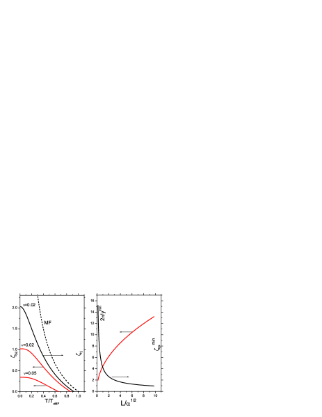
Figure 2: Left panel: dependence of $\zeta_{H}$ and $\zeta_{I}$ on normalized temperature at different $\nu$. Points where $\zeta_{P}=0$ correspond to $\tau_{c}(\nu)$. Dashed line labelled MF corresponds to $\zeta_{MF}=1/\tau-1$. Right panel: equilibrium period of emerging domain structure and parameter $\zeta$ versus dimensionless sample thickness at $\mu_{\perp}=10$ .

These finite values are indeed ”responsible” for the emergence of threshold sample thickness $L_{\rm{tr}}$ beyond mean field approximation. Having dependencies (16), we can solve them numerically for $\zeta_{P}^{\rm{min}}$ (determined above from (15)) to obtain the dimensionless phase transition temperature $\tau_{k}=T_{k}/T_{cMF}$ as a function of critical sample thickness $L_{\rm{cr}}/\sqrt{\alpha}$. In other words, here we have the phase diagram of DMS slab in the coordinates $(T,L)$. This is reported on Fig.3.

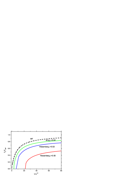
Figure 3: Phase diagram of DMS slab in the coordinates $T,L$. Horizontal asymptotes - $\tau_{c}(\nu)$ similar to Fig.1, $\mu_{\perp}=10$.

The presence of $L_{\rm{cr}}(\nu)$ is clearly seen. The asymptotes for large $L_{\rm{cr}}$ are due to the dependence of equilibrium (i.e. to the ferromagnetic phase without domain structure) phase transition temperature $\tau_{c}=T_{c}/T_{cMF}$ on the concentration ratio $\nu$. Latter dependence is given by the conditions $\zeta_{H}=0$ and $\zeta_{I}=0$ (see (3), (6)) for Heisenberg and Ising models respectively. It was shown in Ref. SS that impurity ferromagnetism in DMS is possible for $0<\nu<\nu_{\rm{cr}}^{P}$ ($P=H,I$, $\nu_{\rm{cr}}^{H}=0.0989$, $\nu_{\rm{cr}}^{I}=0.2473$ SS ) so that $\tau_{c}(\nu_{\rm{cr}})=0$. This means that $\tau_{c}$ decays as $\nu$ grows and the region $(T,L)$, where ferromagnetic domain state exists in DMS, diminishes substantially (compared to the case of ordered ferromagnets) and vanishes as $\nu\to\nu_{\rm{cr}}$.

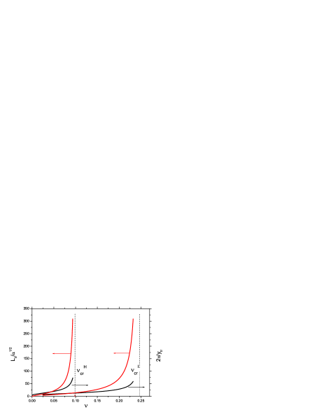
Figure 4: Threshold sample thickness (i.e. that at $T=0$) and corresponding domain structure period as functions of concentration ratio $\nu$ at $\mu_{\perp}=10$. Critical ratios for Heisenberg $\nu_{\rm{cr}}^{H}$ and Ising $\nu_{\rm{cr}}^{I}$ are shown. For mean field approximation (ordered magnet) $\nu_{\rm{cr}}\to\infty$.

Note, that in MF approximation it is very easy to solve (16) analytically to get $\tau_{cMF}=1/(\zeta_{P}+1)$. Resolving the equations (18) for $\zeta_{P}^{\rm{min}}$ we obtain the dependence of threshold thickness on concentration ratio $\nu$. This dependence along with corresponding period of domain structure is shown on Fig.4 for Heisenberg and Ising models. It is seen that as $\nu$ approaches $\nu_{\rm{cr}}$ $L_{\rm{tr}}\to\infty$ so that DMS sample looses its ferromagnetism (both homogeneous and inhomogeneous). The period of domain structure also diverges as $\nu\to$ $\nu_{\rm{cr}}$.

This fact makes it possible to control the critical thickness of DMS sample by changing $\nu$. This, in turn, might give a possibility to engineer the domain structure in nanocrystals od DMS, which is useful for many technical applications (see domains ; DMS1 and references therein). Note that our formalism permits to calculate $\nu_{\rm{cr}}$ and other characteristics of domain structure for any temperature (not only neat $T_{c}$ and sample geometry).

Now we present some numerical estimations. The major problem here is uncertain value of inhomogeneous exchange constant $\alpha$. It can be estimated by the expression land8 $\alpha\approx k_{B}T_{c}a^{2}/(M_{s}\mu_{0})$, where $a=4\AA$ is a typical value of lattice constant for DMS, $M_{s}\approx 50$ mT DMS1 is a saturation magnetization (of localized spin moments) of DMS, $T_{c}=T_{cMF}\approx 100K$ DMS1 is a temperature of transition to homogeneous ferromagnetic state in a mean field approximation, $k_{B}$ and $\mu_{0}$ are Boltzmann constant and Bohr magneton respectively. Evaluation gives $\alpha^{1/2}\sim 200\AA$. From Fig. 4 for $\nu=0.075$ we have threshold sample thickness $L_{\rm{tr}}\sim 50\alpha^{1/2}=10000\AA=1\mu$m and corresponding period of domain structure is $\sim 25\alpha^{1/2}=5000\AA=0.5\mu$m for Heisenberg model. The same values for Ising model occur at $\nu\sim 0.2$. These values are in fair agreement with results of Ref. domains . Moreover, for different $\nu$ we have quite different values of $L_{\rm{tr}}$ and $y_{\rm{tr}}$. This is the base for above discussed domain structure engineering. For our picture to give the quantitative description of experiment in real DMS, the precise experimental determination of inhomogeneous exchange constant $\alpha$ and anisotropy constant $\beta$ is highly desirable.

Here we presented a formalism for the calculation of properties of domain structure in DMS. Our present results about phase diagram of DMS is the simplest application of the formalism. Generally, it permits to calculate all desired properties of domain structure (like the temperature and concentration dependencies of domain structure period and domain walls thickness) in the entire temperature range as well as to account for more complex then slab sample geometries. Latter can be accomplished by applying different from (10) boundary conditions. The external magnetic field can also be easily taken into account. However, far from $T_{k}$ the solution of resulting nonlinear differential equations would require numerical methods.

References

- (1) L.D.Landau,E.M.Lifshits Electrodynamics of continuous media. Wiley, New York, 1984.
- (2) V.V.Tarasenko, E.V.Chenskii, I.E.Dikshtein Sov. Phys. JETP, 43, 1136 (1976).
- (3) T.Dietl, J. König, A.H. MacDonald Phys. Rev. B64, 241201 (2001).
- (4) V.G.Baryakhtar, B.A.Ivanov, Sov. Phys. JETP 45, 789 (1977).
- (5) Recently the ferromagnetism had been discovered in DMS, see M. Tanaka, Semicond. Sci. Tech. 17, 327 (2002). T. Dietl, Semicond. Sci. Tech. 17, 377 (2002).
- (6) T.Dietl, H.Ohno, F.Matsukura Phys. Rev. B63, 195205 (2001).
- (7) Yu. Semenov, V. Stephanovich, Phys. Rev. B67 195203 (2003).
- (8) Yu. G. Semenov, V.A.Stephanovich, Phys. Rev. B66 075202 (2002).
- (9) The equations (3) and (6) have been derived for 3D RKKY interaction between localized magnetic moments in DMS SS2 . For such consideration to be valid, the slab thickness should be more then the range of RKKY interaction ( is Fermi wave vector). For DMS, the typical value of Fermi energy eV. Hence , where is an effective mass of charge carrier, is a free electron mass. So, in our consideration which is the lower limit for plate thickness. However, real plate thickness should be much more then this threshold value. Namely in the phenomenological theory of magnetic domains (see, e.g. TCD and bariv ) the criterion of slab thickness reads . For both above criteria coinside.