Fermi Edge Singularities in Transport through Quantum Dots

Abstract

We study the Fermi-edge singularity appearing in the current-voltage characteristics for resonant tunneling through a localized level at finite temperature. An explicit expression for the current at low temperature and near the threshold for the tunneling process is presented which allows to coalesce data taken at different temperatures to a single curve. Based on this scaling function for the current we analyze experimental data from a GaAs-AlAs-GaAs tunneling device with embedded InAs quantum dots obtained at low temperatures in high magnetic fields.

The generic response of a fermionic many body system to the sudden appearance of a local perturbation is the Fermi-edge singularity (FES). This response can be observed, e.g., in experiments probing X-ray absorption in metals Mahan (1967); Nozières and de Dominicis (1969) or resonant tunneling through localized levels.Matveev and Larkin (1992) In the latter, as depicted in Fig. 1, the Coulomb interaction with a charge in the local state $|\epsilon_{i}\rangle$ acts as a one-body scattering potential for the electrons in the leads.

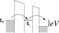
Figure 1: Schematic sketch of the tunneling process through a local state $|\epsilon_{i}\rangle$.

The change of occupation of the local levels during the tunneling process generates sudden changes of this scattering potential leading to characteristic singularities in the $I$–$V$ curves at the corresponding voltage threshold.Geim et al. (1994); Thornton et al. (1998a); Benedict et al. (1998); Hapke-Wurst et al. (2000); Gryglas et al. (2004); Khanin and Vdovin (2005) A theoretical analysis of the low energy response, i.e. in the vicinity of these singularities, at zero temperature is possible using bosonization techniques.Schotte and Schotte (1969) In this approach the response functions can be expressed as correlation functions of boundary changing operators in an equivalent 1+1 dimensional conformal field theory.Affleck and Ludwig (1994) For the tunneling current in the vicinity of the voltage threshold $V_{0}$ this gives a power law,

$$I(V,T=0)\propto(D/e(V-V_{0}))^{\gamma}\,\theta(V-V_{0})\ ,$$ (1)

with a characteristic high energy cutoff $D$ of the order of the band width. The critical exponent $\gamma$ at this threshold is completely determined by the scattering potential and can be expressed in terms of the scattering phase shifts in the channels coupled to the scatterer taken at the associated Fermi momenta.Schotte and Schotte (1969); Nozières and de Dominicis (1969); Matveev and Larkin (1992) The appearance of power laws for the response of the system in this approach is a consequence of the absence of an intrinsic scale in the low-energy theory for this problem.

There are several effects, however, which affect this singularity and therefore obstruct their direct observation: already at zero temperature the finite lifetime of an electron in the local state leads to an intrinsic broadening of this level. Since its energy $\epsilon_{i}$, measured relative to the Fermi energy, depends on the voltage as $\epsilon_{i}\propto e(V-V_{0})$ this broadening directly modifies Eq. (1).Matveev and Larkin (1992) In addition, nonequilibrium effects causing dissipation have to be taken into account for a complete description of the system with a voltage bias across the tunneling barrier. This implies further smoothing of the FES due to the resulting finite lifetime of states in the leads.Bascones et al. (2000); Muzykantskii et al. (2003); Abanin and Levitov (2005) Even without dissipation the response functions such as $I(V)$ of the system are exponentially damped at finite temperature, i.e. away from criticality. However, as the temperature is lowered, Eq. (1) has to be approached, which is reflected by a divergence of the maximum of the measured current as $I(V_{\max},T)\propto T^{-\gamma}$, again limited by the intrinsic broadening of the local level. Here, the critical exponent $\gamma$ is the same as the one governing bias dependence of the $T=0$ response. Finally, the derivation of the expression (1) for the tunneling current in the bosonization approach relies on a linear dispersion of the lead electrons. While this approximation is valid close to the threshold, nonlinearities or fluctuations of the density of states (DOS) due to the presence of impurities in the leads will modify the current for finite detuning $\Delta V=V-V_{0}$ of the voltage. These corrections are a property of the probe and independent of the temperature. Therefore, they can be distinguished from the FES if its dependence on both temperature and voltage, at least at low energies, is known.

Neglecting other than thermal broadening a closed expression for this dependence can be derived for lead electrons with linear dispersion: at finite temperature $T$ and at a finite detuning $\Delta V$ of the voltage from the threshold the response of the system will depend on the ratio $e\Delta V/k_{B}T$ of these energy scales reproducing the power laws mentioned above for zero temperature and at the maximum, respectively. For non-interacting electrons the extension of Eq. (1) for the X-ray absorption problem to finite temperatures can be achieved by taking into account the Fermi distribution for the initial states Ohtaka and Tanabe (1984, 1990) (see also Ref. Yuval and Anderson, 1970). Alternatively, it can be obtained by incorporating temperature in the bosonization procedure of Ref. Schotte and Schotte, 1969. Within the latter approach the analysis is easily generalized to the case of interacting 1D fermions described by the Luttinger Hamiltonian Affleck and Ludwig (1994); Gogolin et al. (1998): the Luttinger parameter $K_{\rho}$ only enters the exponent $\gamma$ in the final expressions (1) and (4). To be specific, we consider a single channel of non-interacting fermions in the emitter of the tunneling device coupled to a local level at the origin. The problem can be formulated as a one-dimensional scattering problem in terms of a left moving (chiral) fermion field $\psi$ on the interval $[-L,L]$ with Fermi velocity $v_{F}$ described by the Hamiltonian (see e.g. Ref. Affleck and Ludwig, 1994)

$${\cal H}=\int\mathrm{d}x\,\left\{iv_{F}\psi^{\dagger}\frac{d}{dx}\psi+\delta(x)U\psi^{\dagger}\psi\,b_{i}^{\dagger}b_{i}\right\}+\epsilon_{i}b_{i}^{\dagger}b_{i}$$ (2)

($b_{i}$ annihilates the electron in the local state). Using Fermi’s golden rule with the tunneling operator $\left(\psi^{\dagger}(0)b_{i}+h.c.\right)$ the current can be expressed in terms of the Green’s function

$$G(t)=\left\langle\left({\cal U}\psi(0,t)\right)^{\dagger}{\cal U}\psi(0,0)\right\rangle_{T}\ .$$ (3)

Here, ${\cal U}(t)$ is the unitary operator describing the change of the boundary condition at $x=0$ due to the tunneling of an electron. It relates the Hamiltonian (2) in the sectors with the local level occupied or empty by means of a canonical transformation.Schotte and Schotte (1969) Representing the fermion $\psi\propto\exp(-i\sqrt{4\pi}\phi)$ in terms of a left-moving boson $\phi(x,t)$ with mode expansion (the zero mode $\phi_{0}$ does not contribute to (3))

$$\phi(x,t)=\phi_{0}+\sum_{m=1}^{\infty}\frac{1}{\sqrt{4\pi m}}\left(a_{m}\mathrm{e}^{-im\pi(x+v_{F}t)/L}+h.c.\right)$$

the Green’s function is ($\delta=U/2v_{F}$ is the Fermi phase shift)

$$G(t)=\exp\left\{\left(1+\frac{\delta}{\pi}\right)^{2}\sum_{m=1}^{\infty}\frac{1}{m}\left[2\left<a_{m}^{\dagger}a_{m}\right>_{T}(\cos{(m\pi t/L)}-1)+\mathrm{e}^{-im\pi t/L}-1\right]\right\}$$

For $T=0$ the ground state expectation value of the bosonic occupation numbers vanishes, $\langle a_{m}^{\dagger}a_{m}\rangle_{0}=0$, and this expression leads directly to (1).Schotte and Schotte (1969); Affleck and Ludwig (1994) At finite temperatures the Bose-Einstein distribution of the bosonic occupation numbers $\langle a_{m}^{\dagger}a_{m}\rangle_{T}$ is used instead.Eggert et al. (1997); Mattsson et al. (1997) Within this approach we obtain ($\gamma=-2\delta/\pi-(\delta/\pi)^{2}$)

$$I(\Delta V,T)\propto\int_{0}^{\infty}\mathrm{d}t\,{\rm e}^{ie\Delta Vt}\,G(t)$$ (4)

$$\quad=\frac{1}{\pi}\mathrm{Im}\left[\left(\frac{i\beta D}{\pi}\right)^{\gamma}\mathrm{B}\left(\frac{1-\gamma}{2}-i\frac{\beta e\Delta V}{2\pi},\gamma\right)\right]$$

for the low temperature response (see also Refs. Ohtaka and Tanabe, 1984, 1990). Here $\beta=1/k_{B}T$ and $\mathrm{B}$ is the beta function.

This expression reproduces the power laws mentioned above: (i) at voltages sufficiently above the threshold, for $e\Delta V\gg k_{B}T$, the power law singularity Eq. (1) emerges from Eq. (4). (ii) For positive $\gamma$, the tunneling current becomes maximal at some finite value of $\beta e\Delta V$ which approaches $0$ for $\gamma\to 1$ and diverges as $\gamma\to 0$. Since a given FES is described by a $T$-independent exponent $\gamma$, this implies that the position of the maximum in the $I$-$V$ curve moves to higher voltage with the temperature $V_{\max}-V_{0}\propto T$. At this maximum, the only temperature dependence of the current is in the pre-factor, i.e. $I_{\max}\propto T^{-\gamma}$. (iii) Finally, for $\gamma\to 0$, i.e.  no scattering of the electrons off the local level irrespective of its occupation, Eq. (4) reduces to a thermally broadened current step $I(\Delta V,T)\propto 1/\left(1+\exp\left(-\beta e\Delta V\right)\right)$.

In the following we apply this result to the analysis of edge singularities observed in tunneling experiments through localized levels in InAs quantum dots in a strong magnetic field. These self-assembled InAs quantum dots are sandwiched between two AlAs tunneling barriers. They have a height of approximately 3 nm and a diameter of $2r_{0}\approx 10-15\,\mathrm{nm}$Hapke-Wurst et al. (2000). The emitter and collector consist of a 15 nm thick undoped GaAs spacer layer followed by a $n$-doped GaAs buffer with graded doping: a 10 nm thick layer of $\mathrm{n^{-}}$ doping ($1\cdot 10^{16}\mathrm{cm}^{-3}$), a 10 nm thick layer of n doping ($1\cdot 10^{17}\mathrm{cm}^{-3}$) and a 1 $\mu$m thick layer of $\mathrm{n^{+}}$ doping ($2\cdot 10^{18}\mathrm{cm}^{-3}$). We have studied two samples with nearly the same growth parameters; only the tunneling barrier thicknesses are different. One has AlAs tunneling barrier thicknesses of 4 and 3 nm and we show here measurements at a magnetic field of 14.9 T. The other sample with more asymmetric barriers (5 and 2 nm) was studied at magnetic fields up to 28 T. In this paper we look at the tunneling direction where the electrons tunnel first through the thicker barrier onto the dot and leave it through the thinner barrier.

The thickness of the spacer layer (15 nm) of the investigated samples was carefully chosen to allow for a description of the emitter as a three dimensional electron gas even at the presented bias voltages, different from the structures used in Ref. Itskevich et al., 1996. A comparison of the $I$-$V$ characteristics to a test sample with a much thicker spacer layer (100 nm) showed distinct differences. For this test sample strong peaks in the $I$-$V$ characteristic due to the formation of 2D subbands in the emitter right before the tunneling barriers evolved. In Ref. Itskevich et al., 1996 such a 2D emitter behavior was also observed for the same 100 nm thickness of the spacer layer. The absence of such peaks in all our samples with a 15 nm spacer layer confirms our assumption of a 3D emitter. Additional support fro this assumption has been given by a detailed analysis of a sample of the wafer with the 4 and 3 nm barriers in Ref. Nauen et al., 2004. Both the current and the measured shot noise showed excellent agreement with the theoretical models for 3D-0D-3D tunneling.

Expression (4) for the tunneling current implies that the $I$–$V$ data taken at different temperatures $T$ – after rescaling the current as $IT^{\gamma}$ and the voltage as $e\Delta V/k_{B}T$ – should lie on a single scaling curve. Here, the only free parameter should be the edge exponent $\gamma$. In practice, however, there are various additional effects to be considered: first, only a fraction $\alpha$ of the total applied voltage drop occurs between the emitter and the quantum dot, i.e. $\epsilon_{i}=\alpha e\Delta V$. The energy-to-voltage conversion factor $\alpha$ can be determined from the thermal broadening of the FES. Second, as already mentioned in the introduction, the local level in the quantum dot has an intrinsic width $\Gamma_{i}$ due to its hybridization with the states in the emitter. The effect of these mechanisms on the broadening of the $I$-$V$ curve is different and non-equilibrium conditionsMuzykantskii et al. (2003); Abanin and Levitov (2005) have to be taken into account for the latter. Here we include both by introducing an effective temperature $k_{B}T^{\prime}\equiv\sqrt{(k_{B}T)^{2}+\Gamma_{i}^{2}}$ in Eq. (4). Based on the theoretical expression we have analyzed data taken with the first sample in a magnetic field of $14.9\,T$ at various temperatures between $0.3$ and $1.0\,K$ (Fig. 2(a)). Due to the Zeeman-splitting of the local level in the dot the FES appear in pairs (see also Refs. Thornton et al., 1998b; Benedict et al., 1998). Hence the data have to be described by the sum of two contributions (4) with different edge exponents $\gamma_{\uparrow}$, $\gamma_{\downarrow}$ but the same conversion factor $\alpha$ and intrinsic broadening $\Gamma_{i}$. Unlike in bulk InAs the Landé factor of the quantum dots is positive.Thornton et al. (1998b); Hapke-Wurst et al. (2000) As a consequence we identify the FES at lower bias voltage with tunneling of spin-$\downarrow$ electrons. Performing a fit to the experimental data we obtain $\gamma_{\uparrow}=0.27$, $\gamma_{\downarrow}=0.46$, $\alpha=0.15$ and $\Gamma_{i}=0.36\,K$. Now, the FES from tunneling of electrons with spin $\downarrow$ (corresponding to the peak in the $I$-$V$ curves at lower bias) can be isolated by subtracting the theoretical contribution from the other spin projection. Rescaling the axes as described above the $I$-$V$ data are indeed seen to collapse onto a single curve given by (4) (see Fig. 2(b)). The scatter observed at higher voltages is caused by fluctuations in the local DOS in the emitter.

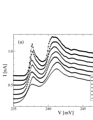
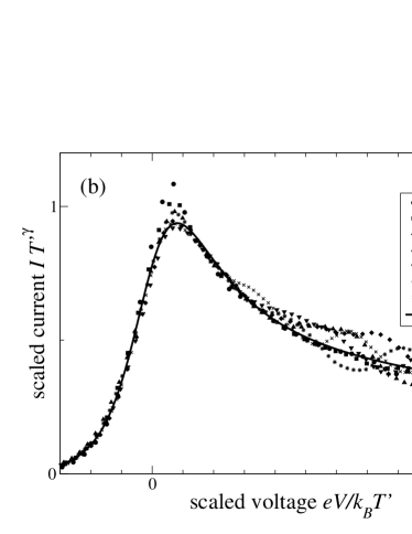
Figure 2: (a) $I$-$V$ characteristics exhibiting the spin-split Fermi edge singularity for a magnetic field of $14.9\,T$ at temperatures $T=0.3\,K$, $0.35\,K$, $0.45\,K$, $0.55\,K$, $0.6\,K$, $0.75\,K$, $1.0\,K$ (for clarity a $T$-dependent offset is added to $I$). (b) Same data for the FES at $V\approx 238\,mV$ with current rescaled as $I\,T^{\prime\gamma}$ vs. voltage in units of the effective temperature $T^{\prime}$ (see main text) for a collapse onto a single curve. The full line is the best fit of Eq. (4) to the data.

As argued above these fluctuations should lead to temperature independent deviations of the experimental data from the theoretical prediction. This behaviour is shown in Fig. 3 where the raw $I$–$V$ data (i.e. without rescaling of the axes) near the Zeeman-split FES at two different temperatures are shown. Taking the ratio of the experimental data to the theoretical fit the temperature independence of the fluctuations in the current becomes manifest, see Fig. 3(b). Although the data show some scatter which is most likely caused by noise in the experimental data, it is astonishing that in all five experimental curves the same small deviation in the theoretical curve can be seen.

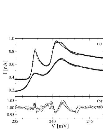
Figure 3: (a) $I-V$ data for a Zeeman-split edge singulartiy at $B=14.9\,T$, $T=0.3\,K$ (upper curve) and $T=1.0\,K$ (lower curve). The dots show the experimental data, the solid line is the theoretical fit. (b) Ratio of experimental data and theoretical fit for temperatures $T=0.3\,K$, $0.45\,K$, $0.6\,K$, $0.75\,K$, $1.0\,K$ showing the (essentially $T$-independent) fluctuations in the local DOS of the emitter.

As has been reported before,Hapke-Wurst et al. (2000) the edge exponents characterizing the FES in the tunneling current depend strongly on the magnetic field. To understand this in terms of the parameters describing the dot and its interaction with the emitter we have to go beyond the generic low-energy Hamiltonian (2): the broadening of the localized level and the Fermi phase shifts determining the edge exponents in (1), (4) need to be computed within a suitable microscopic model. As discussed above the emitter can be described as a 3D electron gas in the half space $z<0$ (see, e.g., Ref Westfahl et al., 1998 for the description of an effective 2D electron system). In the experiment the transverse motion of the electrons is quantized by the magnetic field $B||\hat{z}$. Only the lowest Landau band (LLB), $n=0$, is occupied and the electrons populate one-dimensional channels of given angular momentum $m\geq 0$ with Fermi momentum $\hbar k_{F\sigma}$ for spin projection $\sigma=\uparrow,\downarrow$.Hapke-Wurst et al. (2000) The radial wave functions in these channels, $\psi_{n=0,m}(\rho,\phi)\propto\rho^{m}\exp(-im\phi-\rho^{2}/4\ell_{0}^{2})$, depend on the magnetic field through the magnetic length $\ell_{0}=\sqrt{\hbar/eB}$. In the experiments, $\ell_{0}$ is comparable to the lateral size $r_{0}$ of the quantum dot.

Assuming a Gaussian wave function for the electron on the isolated quantum dot the intrinsic broadening $\Gamma_{i}$ can be computed in perturbation theory from its overlap with the single electron states in the LLB of the leads (in the present geometry the broadening will be dominated by the overlap with the collector states). The field dependence of the wave functions $\psi_{0m}$ leads to a linear growth of the broadening with the magnetic field with a change in slope around $\ell_{0}\approx r_{0}$. This agrees with the qualitative behaviour of $\Gamma_{i}$ as obtained from our fits to the experimental $I$-$V$ data: analyzing the evolution of the FES with the field we find that $\Gamma_{i}$ varies between $0.36\,K$ at $B=14.9\,T$ and $1.5\,K$ at $B=28\,T$. as a consequence, the corresponding lifetimes of particles in the local state are well above the thresholds for the observation of the FES.Main et al. (2000).

Finally, we want to discuss the magnetic field dependence of the edge exponents $\gamma_{\sigma}$ characterizing the Zeeman-split FES. In the tunneling experiment the scattering potential of the dot affects several channels labelled by the angular momentum $m$ and spin $\sigma$ of the electrons. Alternation of the occupation of the quantum dot implies changes $\delta_{m}(k)$ in the Fermi phase shifts experienced by the electrons in channel $m$. As in the simplified model (2) the edge exponents can be expressed in terms of these changes (angular momentum conservation implies that only $m=0$ electrons contribute to the tunneling matrix element) Nozières and de Dominicis (1969)

$$\gamma_{\sigma}=-\frac{2}{\pi}\delta_{0}(k_{F\sigma})-\frac{1}{\pi^{2}}\sum_{m,\sigma^{\prime}}\delta_{m}(k_{F\sigma^{\prime}})^{2}\ .$$ (5)

The scattering potential for the electrons in the emitter is composed from the band bending due to the presence of the semiconductor-insulator interface at $z=0$ and the screened Coulomb potential of a charge on the quantum dot – if it is occupied. In the 1D Landau channels with given angular momentum $m$ both can be described by effective potentials $v\mathrm{e}^{\kappa z}$ decaying exponentially into the emitter with range $\kappa^{-1}$ being the Debye radius. The resulting phase shift picked up by the 1D electrons with momentum $\hbar k$ perpendicular to the boundary is

$$\delta(k)=-\frac{i}{k}\ln\left(\frac{{{}_{0}F_{1}}\left(;1+\frac{2ik}{\kappa},\frac{v}{\kappa^{2}}\right)}{{{}_{0}F_{1}}\left(;1-\frac{2ik}{\kappa},\frac{v}{\kappa^{2}}\right)}\right)$$ (6)

where ${}_{0}F_{1}$ is a hypergeometrical function. For the empty dot the effective potential $v$ is the band bending $v_{b}$ depending on the doping profile. For the charged dot $v=v_{b}+v_{n,m}$ where $v_{n,m}$ is obtained by projecting the screened Coulomb potential $V(\rho,z)$ (see e.g. Ref. Matveev and Larkin, 1992) to the radial wave functions $\psi_{n,m}(\rho,\phi)$ of the electrons in the $n^{\mathrm{th}}$ Landau level Hapke-Wurst et al. (2000). Both the effective potential obtained by this projection and the Fermi momenta $k_{F\sigma}$ in the Landau quantized channels of the emitter are functions of the applied magnetic field. Through Eq. (6) this leads to the strong $B$ dependence of the edge exponents $\gamma_{\sigma}$ observed in experiments with 3D emitter.

In Ref. Hapke-Wurst et al., 2000 the FES was analyzed based on the linear behaviour of (6) for small $k$. In this approximation the difference of the exponents $\gamma_{\uparrow}-\gamma_{\downarrow}$ is proportional to the corresponding Fermi momenta which can be determined from the 1D DOS in the Landau bands (broadened by disorder). As a consequence, the difference of the edge exponents should grow monotonically with $B$. This behaviour is indeed observed in the experiments at sufficiently high magnetic fields $B>B_{c}\approx 20\,T$. Below $B_{c}$, however, the experimental data presented in Ref. Hapke-Wurst et al., 2000 indicate that $\gamma_{\uparrow}-\gamma_{\downarrow}$ changes sign, see also Fig. 4.

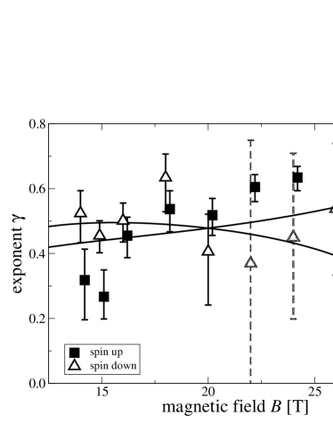
Figure 4: Field dependence of the exponent $\gamma$ for both spin polarisations. For $B>20\,T$ fitting of Eq. (4) to the FES for the minority spin is hampered by its decreasing weight. This results in the large errors displayed for $\gamma_{\downarrow}$. Full lines are theoretical predictions based on the phase shift (6) of the exponentially screened scattering potential.

According to Eq. (5) such a crossing requires that $\delta(k_{F\uparrow})=\delta(k_{F\downarrow})$ for $B_{c}$. Clearly, such a feature requires a non-monotonic $k$-dependence of the Fermi phase shift and can only be captured when the full nonlinear expression (6) for the scattering phase is taken into account. In Fig. 4, we present a theoretical prediction based on this expression. Both Landau level broadening (affecting the field dependence of the Fermi momenta) and bending of the Landau band in the emitter at $z=0$ have to be taken into account. The latter is found to be close to the threshold of formation of a single electron bound state at the interface. This is consistent with our picture that at very high bias voltages a potential well is formed in the emitter close to the barriers. At the same time this limits the validity of the simple description for the scattering potential in the emitter in terms of a decaying exponential used in the derivation of Eq. (6). Within this simple model the qualitative $B$-dependence of the experimental data near $B_{c}$ is reproduced. The splitting of the edge exponents at $B<B_{c}$, however, is underestimated by the prediction. Note that the $z$-dependence of the scattering potential for the electrons in the emitter can, in principle, be determined from the field dependence of the edge exponents. For this, however, they have to be extracted from the experimental data with sufficient accuracy. Here the quality of data is limited in particular by the low weight of the FES for the minority spin $\downarrow$ at fields $B\gtrsim B_{c}$.

In this Paper we have analyzed FES observed in resonant tunneling experiments through InAs quantum dots between 3D leads in strong magnetic fields parallel to the current using both its temperature and bias-voltage dependence. Based on an explicit expression (4) for the $I$-$V$ characteristic of the FES data taken at different temperatures have been collapsed into a single scaling form. From these data the effect of the temperature-independent fluctuations in the local density of states in the emitter on the current has been identified. Furthermore, the parameters describing the interaction between the dot and the lead could be extracted. Based on a microscopic model for the tunneling device the magnetic field dependence of the broadening of the local level on the quantum dot has been described. In addition the exponent characterizing the FES for both spin projections has been computed taking into account the non-linear momentum dependence of the Fermi phase shift (6), reproducing the qualitative behaviour found in the experiment, in particular the change in sign of $\gamma_{\uparrow}-\gamma_{\downarrow}$ at a magnetic field $B\approx 20\,T$. For an improved description, both the effect of non-equilibrium conditionsMuzykantskii et al. (2003); Abanin and Levitov (2005) has to be considered and fine-tuning the scattering potential for the electrons in the emitter used to compute the Fermi phase shift is necessary. The latter would amount to introducing introduction of additional fitting parameters, though. On the other hand, we note that, this potential can be reconstructed in principle from the experimental data provided that the edge exponents can be extracted with sufficient accuracy.