Critical-state effects on microwave losses in type-II superconductors

Abstract

We discuss the microwave energy losses in superconductors in the critical state. The field-induced variations of the surface resistance are determined, in the framework of the Coffey and Clem model, by taking into account the distribution of the vortex magnetic field inside the sample. It is shown that the effects of the critical state cannot generally be disregarded to account for the experimental data. Results obtained in bulk niobium at low temperatures are quantitatively justified.

1 Introduction

Investigation of fluxon dynamics in type-II superconductors is of great interest for both fundamental and applicative aspects. From the basic point of view, it allows measuring the relative magnitude of elastic and viscous forces, which rule the motion regime of the fluxon lattice gittle ; golo ; TALVA ; noi . From the technological point of view, it allows determining the critical current, accounting for the energy losses and investigating the presence of irreversible phenomena, which are important factors for the implementation of superconductor-based devices libromw .

A suitable method to investigate the fluxon dynamics consists in determining the field-induced energy losses at microwave (mw) frequencies, by measuring the surface resistance, $R_{s}$ golo . In the absence of static magnetic fields, the variation with the temperature of the condensed-fluid density determines the temperature dependence of $R_{s}$. On the other hand, the field dependence of $R_{s}$ in superconductors in the mixed state is determined by the presence of fluxons, which bring about normal fluid in their cores, as well as the fluxon motion gittle ; golo ; TALVA ; noi ; CC4 ; BRANDT ; noiPRB .

Coffey and Clem (CC) have elaborated a comprehensive theory for the electromagnetic response of type-II superconductors in the mixed state CC4 , taking into account flux creep, flux flow, and pinning effects in the framework of the two-fluid model. The theory has been developed with two basic assumptions: i) inter-vortex spacing much less than the field penetration depth; ii) uniform vortex distribution in the sample. With these assumptions, the local vortex magnetic field, $B(\textit{{r}})$, averaged over distances larger than several inter-vortex spacings, is spatially uniform. As pointed out by the authors CC4 , the first assumption is valid when the external field, $H_{0}$, is greater than $2H_{c1}$; whereas, the second one does not take into account the magnetic history of the sample.

It is well known that the H - T phase diagram of type-II superconductors is characterized by the presence of the irreversibility line, $H_{irr}(T)$, below which the magnetic properties of the superconducting sample become irreversible. The application of a DC magnetic field smaller than $H_{irr}(T)$ develops a critical state of the vortex lattice BEAN ; KIM and the assumption that $B$ is uniform over the sample is not longer valid. Although the critical state is a metastable energy state, the relaxation times toward the thermal equilibrium state can be much longer than the time during which the measurements are performed yesherun . In this case, the effects of the critical state can be revealed in all the superconducting properties involving the presence of fluxons in the sample.

When the sample is in the critical state, the CC model does not account for the experimental results; for instance, no magnetic hysteresis in the $R_{s}(H_{0})$ curves is expected. Though different authors have justified the hysteretic behavior of the $R_{s}(H_{0})$ curves by considering critical-state effects in the fluxon lattice TINKHAM ; SRIDHAR , the field dependence of the surface resistance for non-uniform flux profile has never been quantitatively investigated.

In this paper, we show that, when the superconducting sample is in the critical state, the CC theory has to be generalized by properly taking into account the flux distribution inside the sample. We suggest a way to considering the critical-state effects. We will show that the $R_{s}(H_{0})$ curve strongly depends on the specific profile of the magnetic induction $B$, determined by the field dependence of the critical current density $J_{c}(B)$. We will report experimental results of the field-induced variations of $R_{s}$ in a niobium bulk sample in the critical state; the results are quite well accounted for by considering a specific $B$ profile inside the sample.

2 The model

In the London local limit, the surface impedance is proportional to the complex penetration depth $\widetilde{\lambda}$ of the em field. In particular,

$$R_{s}=-\mu_{0}\omega~{}\mathrm{Im}[{\widetilde{\lambda}(\omega,B,T)}].$$ (1)

In the CC model, $\widetilde{\lambda}(\omega,B,T)$ is given by

$$\widetilde{\lambda}(\omega,B,T)=\sqrt{\frac{\lambda^{2}(B,T)+(i/2)\widetilde{\delta}_{v}^{2}(\omega,B,T)}{1-2i\lambda^{2}(B,T)/\delta_{nf}^{2}(\omega,B,T)}},$$ (2)

with

$$\lambda(B,T)=\frac{\lambda_{0}}{\sqrt{[1-(T/T_{c})^{4}][1-B/B_{c2}(T)]}},$$ (3)

$$\delta_{nf}(\omega,B,T)=\frac{\delta_{0}}{\sqrt{1-[1-(T/T_{c})^{4}][1-B/B_{c2}(T)]}},$$ (4)

where $\lambda_{0}$ is the London penetration depth at $T=0$ and $\delta_{0}$ is the normal-fluid skin depth at $T=T_{c}$.
$\widetilde{\delta}_{v}$ is the effective complex penetration depth arising from the vortex motion and depends on the relative magnitude of the viscous-drag and restoring-pinning forces. An important parameter, which determines the regime of the fluxon motion, is the so-called depinning frequency, $\omega_{c}$, defined by the ratio between the restoring-force and viscous-drag coefficients. When the frequency of the $em$ wave, $\omega$, is much larger than $\omega_{c}$ the fluxon motion is ruled by the viscous-drag force and the induced $em$ current makes fluxons move in the flux-flow regime, even for $H_{0}<H_{irr}(T)$. On the contrary, for $\omega\ll\omega_{c}$ the motion of fluxons is ruled by the restoring-pinning force. In the following, we will devote the attention to the case in which the vortex lattice moves in the flux-flow regime, where the field-induced energy losses are noticeable. In this case, considering the expression of the viscous coefficient proposed by Bardeen and Stephen BS , it results $\widetilde{\delta}_{v}^{2}=\delta_{0}^{2}B/B_{c2}(T)$. The real part of $\widetilde{\lambda}$ defines the AC penetration depth, $\lambda_{ac}$.

Since the mw losses depend on the local magnetic field $B(\textit{{r}})$, when it is not uniform over the sample, different regions of the sample contribute to the energy losses differently; this should occur when the sample is in the critical state. Generally, the critical state develops at temperatures smaller enough than $T_{c}$, where the pinning effects are significant; in this case, the energy losses are mainly related to the motion of fluxons induced by the mw current. So, a discriminating criterium, to determine in what extent the non-uniform $B$ profile affects the energy losses, consists in evaluating the variation of the DC magnetic induction in the region where fluxons feel the Lorentz force.

Fig. 1 describes the distribution of the fields and the mw current in the two geometries: $\textit{{H}}_{\omega}\|\textit{{H}}_{0}$ (a); $\textit{{H}}_{\omega}\bot\textit{{H}}_{0}$ (b). For the sake of clearness, we limit the analysis to a slab geometry (sample width $w$ and sample height $d$, with $\lambda_{ac}\ll w,d$). We suppose that the static magnetic field, $H_{0}$, is greater than $H_{c1}$ and that the sample is in a critical state à la Bean, i.e. characterized by a field-independent $J_{c}$ BEAN ; however, the analysis applies to any $J_{c}(B)$ dependence. When the mw magnetic field is parallel to the $z$-axis, the mw current penetrates in the surface layers of the sample, of width $\lambda_{ac}$, in the x - y plane. If $\textit{{H}}_{\omega}\|\textit{{H}}_{0}$, only the fluxons in these layers experience the Lorentz force, due to the mw current, and the fluxon lattice undergoes a compressional motion. In Fig. 1 (a) we analyze the regions indicated by the shadowed area. In this case, if the variation of $B$ in these regions is negligible, i.e. $J_{c}\lambda_{ac}\ll\ H_{0}$, the vortex magnetic field can be considered as uniform. A different situation occurs when $\textit{{H}}_{\omega}\bot\textit{{H}}_{0}$, as shown in Fig. 1 (b); in this case, all the vortices present in the sample are involved in the motion, the fluxon lattice undergoes a tilt motion BRANDT , $\lambda_{ac}$ determines the part of the flux line in which the Lorentz force acts; the approximation of $B$ uniform would be proper only if the sample width is such that $J_{c}w\ll\ H_{0}$. So, for bulk samples, it is expected that the specific profile of $B$ strongly affects the $R_{s}(H_{0})$ curve; indeed, different regions of the sample contribute in different extent to the mw energy losses. In the following, we will refer to this field geometry, where the effects of the non-uniform profile of $B$ most affect the $R_{s}(H_{0})$ curve.

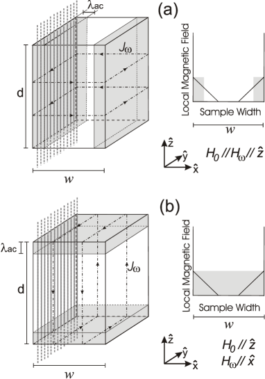
Figure 1: Distribution of the fields and current in two different geometries: $\textit{{H}}_{\omega}\|\textit{{H}}_{0}~{}(a)$; $\textit{{H}}_{\omega}\bot\textit{{H}}_{0}~{}(b)$; the shadowed area indicates the regions of the sample interested by the vortex motion.

Brandt BRANDT has shown that the compressional and tilt motion of the fluxon lattice can be described by the same formalism and the same AC penetration depth results because the compression and tilt moduli are approximately equal. So, the results obtained from the CC model are valid even in the case of tilt motion provided that $B$ is uniform over the region where the Lorentz force is active.

When the DC magnetic induction is not uniform, one can subdivide the sample surface in different regions, in each of them $B(\textit{{r}})$ can be considered uniform. Each part of the surface is characterized by a different $R_{s}$ value, due to the local magnetic induction, and the energy losses of the whole sample are determined by the surface-resistance contributions of each region. The measured surface resistance is an average over the whole sample:

$$R_{s}=\frac{1}{S}\int_{\Sigma}R_{s}(|B(\textit{{r}})|)\,dS\,,$$ (5)

where $\Sigma$ is the sample surface, $S$ is its area and r identifies the surface element; the main contribution comes from the sample regions where $\textit{{H}}_{0}\times\textbf{{J}}_{\omega}\neq 0$.

Usually, in order to disregard the geometrical factor of the sample, the reported experimental results of the surface resistance are normalized to the normal-state value at $T=T_{c}$, $R_{n}$. In the flux-flow regime, in order to calculate $R_{s}/R_{n}$, by Eqs. (1–4), it is necessary to know the ratio $\lambda_{0}/\delta_{0}$ and the upper critical field. Moreover, to take into account the critical-state effects, by Eq. (5), it is also necessary to know the $B$ profile inside the sample, determined by $J_{c}(B)$. We would remark that the analysis can be generalized, in the different motion regimes, by introducing the field dependence of the depinning frequency in $\widetilde{\delta}_{v}(\omega,B,T)$; however, this introduces further fitting parameters.

Fig. 2 shows $R_{s}/R_{n}$ expected in the flux-flow regime as a function of the reduced field, $H_{0}/H_{c2}$, in three different cases. Curve $(a)$ is the one expected from the CC model ($J_{c}=0$). Curves $(b)$ and $(c)$ have been obtained with $J_{c}=J_{c0}$, independent of $B$, and two different values of the full penetration field $H^{*}$ BEAN . All the curves have been obtained with $T=T_{c}/4$ and $\lambda_{0}/\delta_{0}=10^{-2}$; furthermore, for simplicity, it was supposed $H_{c1}=0$. It is evident that, taking into account the distribution of $B$, different field dependencies of $R_{s}$ arise. In particular, a comparison between curves $(b)$ and $(c)$ shows that the greater $H^{*}$, the lower the value of $R_{s}$; this occurs because the induction field of the whole sample decreases on increasing $H^{*}$.

Another important characteristic of the $R_{s}(H_{0})$ curves is the change of concavity occurring at $H_{0}=H^{*}$. When the fluxon lattice moves in the flux-flow regime and $B$ is uniform, it is expected $R_{s}\propto\sqrt{B}$, with $B\approx\mu_{0}H_{0}$, which leads to a negative concavity of the $R_{s}(H_{0})$ curve. For the general case of spatially-dependent flux density, the shape of the $R_{s}(H_{0})$ curve is determined by the external-field dependence of $B$. In particular, when in the whole sample the local magnetic induction linearly depends on the external field a negative concavity of the $R_{s}(H_{0})$ curve is expected. This occurs in the thermal equilibrium state for $H_{0}>2H_{c1}$, as well as in the critical state à la Bean for $H_{0}>H^{*}$ BEAN . The positive concavity of the curves $(b)$ and $(c)$ of Fig. 2, obtained for $H_{0}<H^{*}$, can be qualitatively understood considering that, on increasing the external field from $H_{c1}$ up to $H^{*}$, more and more regions contribute to the mw losses.

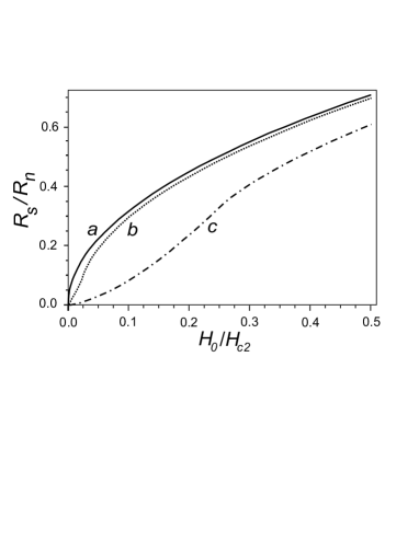
Figure 2: Normalized $R_{s}(H_{0})$ curves, expected in the flux-flow regime, in the different cases: $(a)$ $B$ uniform; $(b)$ critical state à la Bean with $H^{*}=H_{c2}/40$ and $(c)$ $H^{*}=H_{c2}/4$. $T=T_{c}/4$, $\lambda_{0}/\delta_{0}=10^{-2}$.

Figure 3: Expected $R_{s}(H_{0})$ curves, obtained using for the field dependence of the critical current density the laws shown in the inset. $T=T_{c}/4$, $\lambda_{0}/\delta_{0}=10^{-2}$.

When the field dependence of the critical current is taken into account, the shape of the $R_{s}(H_{0})$ curve strongly depends on the $B$ profile due to the specific $J_{c}(B)$ behavior. The field dependence of $J_{c}$ has been widely discussed in the literature both theoretically KIM ; IRIE ; MING and experimentally KOBAYASHI ; DESORBO ; DHALLE ; different behaviors have been suggested. In Fig. 3 we report the expected $R_{s}(H_{0})$ curves, obtained considering different $J_{c}(B)$ laws, along with the curve expected from the CC theory $(a)$; also in this case, we have assumed $H_{c1}=0$. Curve $(b)$ has been obtained using $J_{c}=J_{0}\exp(-B/\Gamma_{0})$, curve $(c)$ with $J_{c}=J_{0}-\alpha~{}B$ and curve $(d)$ with $J_{c}=J_{0}$; the inset shows the corresponding $J_{c}(B)$ laws used. As one can see, the features of the $R_{s}(H_{0})$ curve strongly depend on the profile of $B$ inside the sample. In particular, looking at curve $(b)$, it is evident that when the critical current verges on zero the $R_{s}(H_{0})$ curve approaches the one obtained from the CC theory, as expected. This finding is expected, in any case, for magnetic fields close to $H_{c2}(T)$, where the pinning becomes ineffective and, consequently, $J_{c}\approx 0$.

It is worth noting that we have investigated the effects of the $B$ profile determined by the field dependence of the critical current density on the $R_{s}(H_{0})$ curve, neglecting possible variation of the profile due to the finite dimensions of the superconducting sample. As it is well known, the sheet current, induced near the sample edges, can affect the $B$ profile in the sample brandt2 . These effects are particularly enhanced for thin strips when the DC magnetic field is parallel to the smallest dimension; in this case, a proper $B$ profile has to be considered.

3 Comparison with experiments

In order to study the peculiarities of the $R_{s}(H_{0})$ curve in superconductors in the critical state, we have measured the field-induced variations of $R_{s}$ in bulk Nb at low temperatures, where the pinning effects are significant and a magnetic field smaller enough than $H_{c2}(T)$ develops the critical state of the fluxon lattice. The sample, of dimensions $3.3\times 2.3\times 1.3~{}\mathrm{mm^{3}}$, has been cut from a Tokyo Denkai batch with $\mathrm{RRR}=300$ and undergoes a superconducting transition at $T_{c}\approx 9.2$ K. We have studied the Nb because the depinning frequency GOLOSOVSKY is small enough to suppose that the mw current induces the fluxon lattice moving in the flux-flow regime; furthermore, our experimental apparatus allows reaching DC magnetic fields of the order of $H_{c2}$.

The mw surface resistance has been measured using the cavity-perturbation technique TRUNIN . A copper cavity, of cylindrical shape with golden-plated walls, is tuned in the TE₀₁₁ mode, resonating at 9.6 GHz. The cavity is placed between the poles of an electromagnet, which generates magnetic fields up to $\sim 1~{}\mathrm{T}$. The sample is located in the center of the cavity where the mw magnetic field is maximum. The field geometry is that shown in Fig. 1 (b) and, therefore, the mw current induces a tilt motion of the whole fluxon lattice. The $R_{s}$ values are determined measuring the variation of the quality factor of the cavity, induced by the sample, by an $hp$-8719D Network Analyzer.

In order to check the presence of the critical state in the sample, we have measured the field-induced variations of $R_{s}$ by cycling the DC magnetic field from zero to the maximum value available in our experimental apparatus and back, at different values of the temperatures. Up to 2 K below $T_{c}$, $R_{s}$ exhibits a magnetic hysteresis that disappears for $H_{0}$ higher than a certain value, depending on the temperature. In particular, in the range of temperatures $T\approx 2\div 4$ K the hysteretic behavior is detectable up to $H_{0}\approx 0.4$ T; at higher temperatures, the field range in which the hysteresis is present shrinks; eventually, for $T>7$ K, the $R_{s}(H_{0})$ curve becomes reversible in the whole range of fields investigated. These findings confirm that, at temperatures smaller enough than $T_{c}$, the external field develops a critical state in the fluxon lattice. Furthermore, in the field range in which the hysteresis is observed, $R_{s}$ does not exhibit any detectable time evolution, from the instant in which the field value has been set, ensuring that the critical state does not relax during the time in which the measurements are performed. The hysteretic behavior of microwave surface resistance will be discusses in a forthcoming paper; in this paper, we are interested to investigate the critical-state effects on the $R_{s}(H_{0})$ curve at increasing magnetic field, and to test the method we suggest for taking into account the not uniform $B$ distribution in the sample.

Fig. 4 shows the field-induced variations of $R_{s}$, obtained in the Nb sample at the two temperatures $T=4.2$ K (a) and $T=2.2$ K (b). In the figure, $\Delta R_{s}(H_{0},T)\equiv R_{s}(H_{0},T)-R_{res}$, where $R_{res}$ is the residual mw surface resistance at $T=2.2$ K and $H_{0}=0$; the data are normalized to the maximum variation, $\Delta R_{s}^{max}\equiv R_{n}-R_{res}$. $R_{s}$ does not show any variation as long as $H_{0}$ reaches a certain value that can be identified as the first penetration field, $H_{p}$. From the data, we obtain $H_{p}(4.2~{}\mathrm{K})\approx 52$ mT and $H_{p}(2.2~{}\mathrm{K})\approx 57$ mT; these values are smaller than those reported in the literature for the lower critical field in Nb superconductor because of the demagnetization effects. The dashed and pointed lines are the curves expected from the CC model; the continuous lines are those obtained in the framework of our model; all the expected curves are plotted for $H_{0}>H_{p}$. Since the depinning frequency reported in the literature for Nb are smaller than 100 MHz GOLOSOVSKY , we have assumed that fluxons move in the flux-flow regime. The essential parameters to calculate the expected curves are: $\lambda_{0}/\delta_{0}$, $H_{c2}(T)$ and the $B$ profile inside the sample. According to the results reported in the literature PADAMSEE ; GOLUBOV , we have used $\lambda_{0}/\delta_{0}=3\times 10^{-2}$; however, for $T<T_{c}$/2 the expected results are little sensitive to variations of this parameter. $H_{c2}(4.2~{}\mathrm{K})$ has been determined experimentally and it results 1.1 T; the value of the upper critical field at $T=2.2$ K has been used as fitting parameter and we have found $H_{c2}(2.2~{}\mathrm{K})=1.8~{}\mathrm{T}$. To take into account the presence of the critical state, we have used a field dependence of $J_{c}$ similar to that reported by Cline et al. CLINE for Nb crystals; in particular, it has been used a linear field dependence of $J_{c}$ at low fields, followed by an exponential decrease for $H_{0}\geq H^{\prime}$. The value of $H^{\prime}$ has been considered as fitting parameter; the best-fit curves (continuous lines of Fig. 4) have been obtained using $H^{\prime}(4.2~{}\mathrm{K})=0.35~{}\mathrm{T}$ and $H^{\prime}(2.2~{}\mathrm{K})=0.5~{}\mathrm{T}$. The $B$ profiles, obtained on increasing $H_{0}$, which come out from the used $J_{c}(B)$ laws, are shown in the insets. The full penetration fields calculated from the $B$ profiles are $H^{*}(4.2~{}\mathrm{K})=0.41~{}\mathrm{T}$ and $H^{*}(2.2~{}\mathrm{K})=0.56~{}\mathrm{T}$.

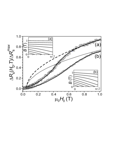
Figure 4: Normalized field-induced variations of $R_{s}$ at: $T=4.2~{}\mathrm{K}~{}(a)$ and $T=2.2~{}\mathrm{K}~{}(b)$. Symbols are the experimental results. Dashed and pointed lines have been obtained from the CC model using $\lambda_{0}/\delta_{0}=3\times 10^{-2}$; $H_{c2}(2.2~{}\mathrm{K})=1.8~{}\mathrm{T}$ and $H_{c2}(4.2~{}\mathrm{K})=1.1~{}\mathrm{T}$. The continuous lines are the best-fit curves of the data, obtained using the same values of $\lambda_{0}/\delta_{0}$ and $H_{c2}(T)$ and the $B$ profiles shown in the insets.

As one can see, in the whole range of $H_{0}$ investigated the experimental results are quite well accounted for by considering the $B$ distribution inside the sample. At low fields, the non-uniform $B$ profile affects to a detectable extent the energy losses, giving rise to the positive concavity of the $R_{s}(H_{0})$ curve. On increasing $H_{0}$, the slope of the field profile decreases; the effects of the non-uniform $B$ distribution become less and less important; eventually, when $B$ becomes roughly uniform over the sample, the observed behavior of $R_{s}(H_{0})$ is consistent with that expected from the CC model.

It has been experimentally observed will , and theoretically justified brandt3 , that, in samples of finite dimensions, the application of an AC magnetic field normal to the DC field gives rise to a ”shaking” of the fluxon lattice, inducing relaxation toward the uniform distribution. The process is particularly relevant when the amplitude of the AC field is of the order of the full penetration field. In mw measurements with the cavity perturbation technique, the amplitude of the mw magnetic field is, usually, much smaller than 1 Gauss, so the process can play a role only in very thin samples or in proximity of the irreversibility line, where the critical current is very small. Of course, if this process occurs, the mw field assists fluxon distributing uniformly in the sample and, consequently, a variation of the $R_{s}(H_{0})$ curve is expected.

Another effect we have neglected is the deformation of the $B$ profile near the edges of the sample brandt2 ; however, the measured $R_{s}$ value is due to the average response of the whole sample, and, therefore, our measurements do not allow estimating in what extent this effect influences the experimental curves. On the other hand, the results reported in Fig. 4 show that the $B$ profiles shown in the insets are suitable to well account for the experimental data.

4 Conclusion

In summary, we have studied the field-induced energy losses in superconductors in the critical state. We have shown that the distribution of the local vortex magnetic field in the sample can strongly affect the field dependence of the mw surface resistance. The analysis has been carried out for the field geometry in which the mw current induces a tilt motion of the fluxon lattice; indeed, in this case, the non-uniform flux distribution most affects the $R_{s}(H_{0})$ curve. The expected curves have been obtained supposing that the fluxons move in the flux-flow regime, where the field-induced energy losses are relevant even for applied fields much smaller than $H_{c2}$; on the other hand, the analysis can be easily extended to a more general case, provided that the field dependence of the depinning frequency is known. We have highlighted that the effects of the critical state on the mw energy losses cannot generally be disregarded to account for the experimental data. Experimental results of field-induced variations of $R_{s}$ in a Nb bulk sample at low temperatures have been justified quite well in the framework of our model.

The authors are very glad to thank G. Lapis and G. Napoli for technical assistance.

References

- (1) J. I. Gittleman and B. Rosenblum, Phys. Rev. Lett. 16, 734 (1966).
- (2) M. Golosovsky, M. Tsindlekht, and D. Davidov, Supercond. Sci. Technol. 9, 1 (1996) and Refs. therein.
- (3) J. Owliaei, S. Shridar, and J. Talvacchio, Phys. Rev. Lett. 69, 3366 (1992).
- (4) S. Fricano, M. Bonura, M. Li Vigni, Klinkova, and Barkovskii, Eur. Phys. J. B 41, 313 (2004).
- (5) H. Weinstock and M. Nisenoff (eds.), Microwave Superconductivity, NATO Science Series, Series E: Applied Science - Vol. 375, Kluwer: Dordrecht 1999.
- (6) M. W. Coffey and J. R. Clem, Phys. Rev. Lett. 67, 386 (1991); Phys. Rev. B 45, 9872 (1992); 45, 10527 (1992).
- (7) E. H. Brandt, Phys. Rev. Lett. 67, 2219 (1991).
- (8) A. Agliolo Gallitto, I. Ciccarello, M. Guccione, M. Li Vigni,and D. Persano Adorno, Phys. Rev. B 56, 5140 (1997).
- (9) C. P. Bean, Phys. Rev. Lett. 8, 250 (1962).
- (10) Y. B. Kim, C. F. Hempstead, and A. R. Strnad, Phys. Rev. Lett. 9, 306 (1962).
- (11) Y. Yesherun, A. P. Malozemoff, A. Shaulov, Rev. Mod. Phys. 68, 911 (1996), and Refs. therein.
- (12) L. Ji, M. S. Rzchowski, N. Anand, and M. Tinkham, Phys. Rev. B 47, 470 (1993).
- (13) Balam A. Willemsen, J. S. Derov, and S. Sridhar, Phys. Rev. B 56, 11989 (1997).
- (14) J. Bardeen and M. J. Stephen, Phys. Rev. 140, A1197 (1965).
- (15) F. Irie and K. Yamafuji, J. Phys. Soc. Jpn. 23, 255 (1967).
- (16) Ming Xu, Donglu Shi, and Ronald F. Fox, Phys. Rev. B 42, 10773 (1990).
- (17) T. Kobayashi, T. Kimura, J. Shimoyama, K. Kisho, K. Kitazawa, and K. Yamafuji, Physica C 254, 213 (1995).
- (18) W. DeSorbo, Phys. Rev. 134, A1119 (1964).
- (19) M. Dhallé, P. Toulemonde, C. Beneduce, N. Musolino, M. Decroux, and R. Flukiger, Physica C 363, 155 (2001).
- (20) E. H. Brandt, Phys. Rev. B. 54, 4246 (1996).
- (21) M. R. Trunin, Physics-Uspekhi 41, 843 (1998).
- (22) H. E. Cline, C. S. Tedmon, Jr., and R. M. Rose, Phys. Rev. 137, A1767 (1965).
- (23) M. Golosovsky, M. Tsindlekht, H. Chayet, and D. Davidov, Phys. Rev. B 50, 470 (1994).
- (24) A. A. Golubov, M. R. trunin, A. A. Zhukov, O. V. Dolgov, and S. V. Shulga, J. Phys. I France 6, 2275 (1996).
- (25) H. Padamsee, Supercond. Sci. Technol. 14, R28 (2001).
- (26) M. Willemin, C. Rossel, J. Hofer, H. Keller, A. Erb, E. Walker, Phys. Rev. B. 58, R5940 (1998).
- (27) E. H. Brandt and G. P. Mikitik, Phys. Rev. Lett. 89, 027002 (2002); G. P. Mikitik and E. H. Brandt, Phys. Rev. B. 67, 104511 (2003).