Charge order in the Falicov-Kimball model

Abstract

We examine the spinless one-dimensional Falicov-Kimball model (FKM) below half-filling, addressing both the binary alloy and valence transition interpretations of the model. Using a non-perturbative technique, we derive an effective Hamiltonian for the occupation of the localized orbitals, providing a comprehensive description of charge order in the FKM. In particular, we uncover the contradictory ordering roles of the forward-scattering and backscattering itinerant electrons: the latter are responsible for the crystalline phases, while the former produces the phase separation. We find an Ising model describes the transition between the phase separated state and the crystalline phases; for weak-coupling we present the critical line equation, finding excellent agreement with numerical results. We consider several extensions of the FKM that preserve the classical nature of the localized states. We also investigate a parallel between the FKM and the Kondo lattice model, suggesting a close relationship based upon the similar orthogonality catastrophe physics of the associated single-impurity models.

I Introduction

The Falicov-Kimball Model (FKM) describes the interaction between conduction electrons and localized atomic orbitals. The Hamiltonian of the one-dimensional (1D) FKM for spinless Fermions is written

$${\cal{H}}_{\text{\tiny{FKM}}}=-t\sum_{j}\left\{c^{\dagger}_{j}c_{j+1}+\mbox{H.c.}\right\}+\epsilon_{f}\sum_{j}n^{f}_{j}+G\sum_{j}n^{f}_{j}n^{c}_{j}$$ (1)

where $t>0$ is the conduction ($c$) electron hopping, $\epsilon_{f}$ is the energy of the localized $f$-electron level, and $G$ is the on-site interorbital Coulomb repulsion. The concentration of electrons is fixed at $n=(1/N)\sum_{j}\left\{\langle{n^{f}_{j}}\rangle+\langle{n^{c}_{j}}\rangle\right\}$ where $N$ is the number of sites. In this work we consider only the case $n<1$. We work throughout at zero temperature $T=0$.

The FKM was originally developed as a minimal model of valence transitions: continuous or discontinuous changes in the occupation of the $f$ orbitals (the atomic “valence”) were observed when varying the coupling $G$ or the $f$-level energy $\epsilon_{f}$. FKMoriginal Since only the distribution of electrons across the two orbitals is of interest, the model has traditionally been studied for spinless fermions. These early works, however, neglected an important feature of ${\cal{H}}_{\text{\tiny{FKM}}}$: the occupation of each $f$-orbital is a good quantum number and so may be replaced in Eq. (1) by its expectation value $n^{f}_{j}\rightarrow\langle{n^{f}_{j}}\rangle=0,1$. It was quickly realized that in many physical systems displaying a valence instability (e.g. SmB₆ and Ce), this is an inappropriate idealization. Instead of a mixture of atoms with different integer valence, in these materials each atomic orbital exists in a superposition of its different occupancy states. LRP81 Although the FKM was modified to include this quantum behaviour by the addition of a $c$-$f$ hybridization term, Vfinite ; Liu&Ho it has now been superseded as a model of valence transitions by the periodic Anderson model. C86

The FKM was reinvented by Kennedy and Lieb in 1986 as a simple model of a binary alloy. KL86 Assuming fixed $c$- and $f$-electron populations, the sites with occupied and unoccupied $f$ orbitals may be regarded as different atomic species A and B respectively. The Coulomb repulsion $G$ is interpreted as the difference between the single-particle energies of the two atoms. For this so-called crystallization problem (CP), the ground state is defined as the configuration of the two atomic species ($f$ electrons) that minimizes the energy of the $c$ electrons. The ordering of the different atomic constituents in a binary alloy is an important theoretical and experimental problem: in realistic systems a large range of ordered structures are observed, although the electronic mechanisms responsible for these phases have remained largely obscure. deFontaine ; D:OPSA By studying a simple model such as the FKM, some insight into the origin of the charge order might be obtained.

Kennedy and Lieb analyzed Eq. (1) for a bipartite lattice at half-filling and equal concentrations of $c$ and $f$ electrons. In the limit of $T=0$ and strong-coupling, they proved that the $f$ electrons occupied one sublattice only, the so-called checkerboard state. This crystalline state is, however, unique to half-filling: for all other fillings, the $G\rightarrow\infty$ ground state is the so-called segregated (SEG) phase. seg1D ; segND The SEG phase is characterized by the $f$ electrons forming a single cluster, arranged in such a manner as to present the smallest perimeter with the rest of the lattice, which is occupied by the $c$ electrons. These strong-coupling results hold for all dimensions $d$. At weak- and intermediate-coupling, the situation is considerably more complicated: for $d=1$, both analytic GLM93 ; FGM96 and numeric FF90 ; GUJ94 ; GJL96 studies have revealed a myriad of different crystalline orderings of the $f$ electrons. The SEG phase is also realized, but not as ubiquitously as at strong-coupling. Intriguingly, for certain $c$- and $f$-electron fillings, the system is unstable towards a special phase-separated state, where the ground state configuration of the localized electrons is a mixture of a crystalline phase and the state with completely empty or full localized orbitals. FB93 ; FGM96 ; GJL96 Work in higher dimensions has revealed similar behaviour; 2D the understanding of the $d\rightarrow\infty$ limit phase diagram is particularly advanced. DMFT

Contemporary with Kennedy and Lieb’s work, Brandt and Schmidt introduced the FKM as an exactly-solvable model of a “classical” valence transition. BS The distribution of the electron weight between the two orbitals is not fixed, but instead determined by the interations. Quantum effects such as superposition of orbital states are ignored: as in the CP, the valence transition problem (VTP) is also concerned with the configuration adopted by the available $f$ electrons. Despite the similarity between the two interpretations, apart from the $d\rightarrow\infty$ limit DMFT and the $d=1$ half-filling case, F95a ; F95b very little is known about the ground states of the VTP. Since the ordered configurations found for the CP occur over a wide range of different fillings and coupling strengths, we can nevertheless expect that the VTP has a similarly rich phase diagram.

Although an impressive catalog of charge-ordered phases has been assembled for the 1D FKM, only the weak-coupling crystalline phases are easily explicable as due to the $c$-electron backscattering off the localized orbitals. The mechanism responsible for the weak-coupling segregated and phase separated states remains unknown; the competition between crystallization and the segregation is also poorly comprehended. In this paper, we expand upon our previous work, BG06 outlining a comprehensive theory of the charge order in the FKM, with particular emphasis on the phase separation.

To describe the $c$ electrons, we use the well-known non-perturbative bosonization technique, specially adapted to account for the presence of localized orbitals. We then canonically transform the bosonized FKM, rewriting the Hamiltonian in a new basis that reveals the origin of the phase separation to be the $c$-electron delocalization. Such a mechanism has previously been proposed to account for the ferromagnetic phase in the 1D Kondo lattice model (KLM), HG pointing to a nontrivial connection between the two models based upon orthogonality-catastrophe physics. After simple manipulation of the transformed Hamiltonian we decouple entirely the $c$ and the $f$ electrons, obtaining an Ising-like effective Hamiltonian describing only the occupation of the $f$ orbitals. The competition between the segregation and crystallization is clearly evident in this effective model: at weak-coupling we find the backscattering crystallization dominates the physics; with increasing $G$, however, the electron delocalization drives the system into the SEG phase. We verify that both crystallization and segregation are present also in the VTP.

Our paper is arranged as follows: in Sec. II we give a brief outline of our bosonization procedure, and present ${\cal{H}}_{\text{\tiny{FKM}}}$ in the bosonic form. We proceed to a description of the canonical transform in Sec. III, including a discussion of the resulting terms. We argue in Sec. IV for the derivation of the effective Hamiltonian for the localized $f$ orbitals from the canonically-transformed Hamiltonian; this is subsequently used in Sec. V to interpret the numerically-determined phase diagrams for the CP (Sec. V.1) and the VTP (Sec. V.2). We also present a brief analysis of several extensions of the FKM in Sec. VI, specifically intraorbital nearest-neighbour interactions and the introduction of spin, focusing upon possible alteration of the CP phase diagram. We conclude in Sec. VII with a summary of our results and the outlook for further work.

II Bosonization

The technique of bosonization has for many years been used to study the critical properties of one-dimensional many-electron systems. G:QP1D It relies upon the remarkable fact that an effective low-energy description of such systems may be constructed in terms of bosonic fields: this representation is usually much easier to manipulate than the equivalent fermionic form. The bosonization of a tight-binding Hamiltonian is often performed in the continuum limit where the lattice spacing $a\rightarrow 0$; G:QP1D this approach is, however, inappropriate for systems involving localized electron states. For the itinerant electrons in the FKM, however, the usual bosonization approach can be generalized to account for the presence of the localized $f$ electrons. As explained in LABEL:G04, this is accomplished by imposing a finite cut-off $\alpha>a$ on the wavelength of the bosonic density fluctuations. Below we summarise our methodology.

The Bose representation is most conveniently written in terms of the dual Bose fields. For a system of length $L\gg{a}$ we have

$$\phi(x_{j}) = -i\sum_{\nu}\sum_{k\neq 0}\frac{\pi}{kL}\rho_{\nu}(k)\Lambda_{\alpha}(k){e}^{ikx_{j}}$$ (2)

$$\theta(x_{j}) = i\sum_{\nu}\sum_{k\neq 0}\nu\frac{\pi}{kL}\rho_{\nu}(k)\Lambda_{\alpha}(k){e}^{ikx_{j}}$$ (3)

At the core of the bosonization technique are the chiral density operators

$$\rho_{\nu}(k)=q\sum_{0<\nu{k^{\prime}}<\pi/a}c^{\dagger}_{k^{\prime}-k}c_{k^{\prime}}$$ (4)

which describe coherent particle-hole excitations about the right and left Fermi points: as subscript (otherwise) we have $\nu=R(+)$, $L(-)$ respectively. The $\rho_{\nu}(k)$ are the basic bosonic objects, obeying the standard commutation relations

$$\left[\rho_{\nu}(k),\rho_{\nu^{\prime}}(k^{\prime})\right]_{-}=\delta_{\nu,\nu^{\prime}}\delta_{k,-k^{\prime}}\frac{\nu{kL}}{2\pi}$$ (5)

for wave vectors $|k|<\frac{\pi}{\alpha}$. The physical significance of the Bose fields is as potentials: $\partial_{x}\phi(x_{j})$ and $\partial_{x}\theta(x_{j})$ are respectively proportional to the departure from the noninteracting values of the average electron density and current at $x_{j}$.

The bosonic wavelength cut-off is enforced in Eq. (2) and Eq. (3) by the function $\Lambda_{\alpha}(k)$ which has the approximate form

$$\Lambda_{\alpha}(k)\approx\left\{\begin{array}[]{cl}1&|k|<\frac{\pi}{\alpha}\\ 0&\text{otherwise}\end{array}\right.$$ (6)

We expect that $\Lambda_{\alpha}(k)$ is a smoothly varying function of $|k|$, reflecting the gradual change in the nature of the density fluctuations. We require, however, that $\Lambda_{\alpha}(k)$ be not too ‘soft’, i.e. $\Lambda^{m}_{\alpha}(k)\approx\Lambda_{\alpha}(k)$ for $m=2,3,4$. The cut-off essentially ‘smears’ the Bose fields over the length $\alpha$ below which the density operators do not display bosonic characteristics. The commutators of the Bose fields reflect this smearing, with important consequences for our analysis:

$$\left[\phi(x_{j}),\theta(x_{j^{\prime}})\right]_{-} = \frac{i\pi}{2}{\text{sgn}_{\alpha}(x_{j^{\prime}}-x_{j})}$$ (7)

$$\left[\partial_{x}\phi(x_{j}),\theta(x_{j^{\prime}})\right]_{-} = -i\pi\delta_{\alpha}(x_{j^{\prime}}-x_{j})$$ (8)

$\text{sgn}_{\alpha}(x)$ and $\delta_{\alpha}(x)$ are the $\alpha$-smeared sign and Dirac delta functions respectively. The precise form of these functions depends upon $\Lambda_{\alpha}(k)$ [see Sec. III.1].

As is customary, we linearize the $c$-electron dispersion about the two Fermi points. This allows a decomposition of the $j$-site annihilation operator in terms of states in the vicinity of $k_{F}$ (the right-moving fields) and $-k_{F}$ (the left-moving fields):

$$c_{j}\approx c_{Rj}e^{ik_{F}{x_{j}}}+c_{Lj}e^{-ik_{F}{x_{j}}}$$

Remarkably, the density operators $\rho_{\nu}(k)$ generate the entire state space of the linearized Fermion Hamiltonian. A Bose representation for the $c_{\nu{j}}$ may then be derived by requiring that it correctly reproduces the Fermion anticommutators and noninteracting expectation values. This leads to the fundamental bosonization identity

$$c_{\nu{j}}=\sqrt{\frac{{A}a}{\alpha}}\hat{F}_{\nu}\exp\left(-i\nu\left[\phi(x_{j})-\nu\theta(x_{j})\right]\right)$$ (9)

We note that this identity is only rigorously true in the long-wavelength limit; Eq. (9) may not correctly reproduce the short-range ($<{\cal{O}}(\alpha)$) properties of the $c_{\nu{j}}$. The dimensionless parameter $A$ is a normalization constant dependent upon the cut-off function. The Klein factors $\hat{F}_{\nu}$ obey the simple algebra:

$$\left[\hat{F}_{\nu},\hat{F}_{\nu^{\prime}}\right]_{+}=2\hat{F}_{\nu}\hat{F}_{\nu}\delta_{\nu,\nu^{\prime}},\qquad\left[\hat{F}_{\nu},\hat{F}^{\dagger}_{\nu^{\prime}}\right]_{+}=2\delta_{\nu,\nu^{\prime}}$$ (10)

The Klein factors act as “ladder operators”: since the Bose fields only operate within subspaces of constant particle number we require operators to move between these different subspaces if we are to regard equation Eq. (9) as an operator identity. That is, $\hat{F}_{\nu}$ may be thought of as lowering the total number of $\nu$-moving electrons by one.

Using standard field-theory methods, the bosonization identity Eq. (9) may be used to derive the Bose representation for any string of Fermion operators. Of particular note is the representation for the $j$-site occupancy operator, $n^{c}_{j}$:

$$n^{c}_{j} \approx \sum_{\nu,\nu^{\prime}}c^{\dagger}_{\nu{j}}c_{{\nu^{\prime}}j}e^{-i(\nu-\nu^{\prime})k_{F}{x_{j}}}$$ (11)

$$= n^{c}_{0}-\frac{a}{\pi}\partial_{x}\phi(x_{j})+\frac{Aa}{\alpha}\sum_{\nu}\hat{F}^{\dagger}_{\nu}\hat{F}_{-\nu}e^{i2\nu\phi(x_{j})}e^{-i2\nu{k}_{F}x_{j}}$$

The first term on the RHS, $n^{c}_{0}$, is the noninteracting $c$-electron concentration; the second term gives the departure from this value in the interacting system and is due entirely to forward scattering ($\nu\rightarrow\nu$ processes); the third term is the first order backscattering ($\nu\rightarrow-\nu$ processes) correction. Higher order backscattering corrections are neglected.

II.1 The Hamiltonian in Boson Form

We bosonize the FKM Hamiltonian using the above methodology. Since only the itinerant $c$ electrons can be bosonized, we require that there be a finite population in the noninteracting $c$-electron band. For the CP this simply requires us to assume finite concentrations of the two species, $n^{c}$ and $n^{f}$ for the $c$ and $f$ electrons respectively, which do not change with the addition of the interaction term. For the VTP, we impose the condition that the $f$-level coincides with the Fermi energy in the noninteracting system: as we consider only the case $n<1$, we limit ourselves to $-2t<\epsilon_{f}<-2t\cos(\pi{n}/a)$. For $\epsilon_{f}$ outside this range, our bosonization approach does not work. We discuss this in more detail in Sec. V.2.

Before bosonizing the Coulomb interaction, we re-write the $f$-electron occupation in terms of pseudospin-$\tfrac{1}{2}$ operators, $n^{f}_{j}-\tfrac{1}{2}=\tau^{z}_{j}$. In the pseudospin representation, spin-$\uparrow$ at site $j$ indicates an occupied $f$-orbital and vice versa. For the CP, the condition of constant $f$-electron concentration then translates into a fixed pseudospin magnetization $m^{z}=n^{f}-\frac{1}{2}$. The use of the pseudospins will considerably simplify the subsequent manipulations. We re-write the Coulomb interaction

$$G\sum_{j}n^{f}_{j}n^{c}_{j}=G\sum_{j}\tau^{z}_{j}n^{c}_{j}-\tfrac{1}{2}{G}\sum_{j}\tau^{z}_{j}+\text{const.}$$ (12)

We have used the requirement of constant total electron concentration to obtain the second term. Substituting Eq. (11) into Eq. (12), we obtain the bosonized form of the FKM Hamiltonian

$${\cal{H}}_{\text{\tiny{FKM}}} = \frac{v_{F}{a}}{2\pi}\sum_{j}\left\{\left(\partial_{x}\phi(x_{j})\right)^{2}+\left(\partial_{x}\theta(x_{j})\right)^{2}\right\}+G\left(n^{c}_{0}-\tfrac{1}{2}\right)\sum_{j}\tau^{z}_{j}$$ (13)

$$-\frac{Ga}{\pi}\sum_{j}\tau^{z}_{j}\partial_{x}\phi(x_{j})+\frac{GAa}{\alpha}\sum_{\nu,j}\tau^{z}_{j}\hat{F}^{\dagger}_{\nu}\hat{F}_{-\nu}e^{i2\nu\phi(x_{j})}e^{-i2\nu{k}_{F}x_{j}}$$

For $c$-electron concentration $n^{c}$, the Fermi velocity is defined $v_{F}=-2ta\sin(k_{F}{a})$ where $k_{F}={\pi}n^{c}/a$. Note that the parameter $\epsilon_{f}$ only enters into Eq. (13) indirectly through $v_{F}$ and $k_{F}$. Since the Klein factor products in the backscattering corrections [the last term in Eq. (13)] commute with the Hamiltonian, we replace them by their expectation value, $\hat{F}^{\dagger}_{\nu}\hat{F}_{-\nu}=\langle\hat{F}^{\dagger}_{\nu}\hat{F}_{-\nu}\rangle=1$.

III The Canonical Transform

The work on the CP has established that the $c$ electrons mediate interactions between the $f$ electrons via the interorbital Coulomb repulsion. Very little, however, is known about the character of these interactions: here we seek to reveal the electronic origins of the charge order by rotating the Hilbert space basis to decouple the $c$ and $f$ electrons. We apply a lattice generalization of the canonical transform used by Schotte and Schotte in the X-ray edge problem (XEP): SS69

$$\hat{U}=\exp\left\{i\frac{Ga}{\pi v_{F}}\sum_{j^{\prime}}\tau^{z}_{j}\theta(x_{j^{\prime}})\right\}$$ (14)

The canonical transform bears a close resemblance to the transform used by Honner and Gulácsi in their analysis of the KLM. HG This resemblance is not coincidental, but instead points to a fundamental similarity between the FKM and KLM which we explore below.

A major advantage of the Bose representation is that the transformation of the Bose operators under Eq. (14) may be calculated exactly using the Baker-Hausdorff formula. This allows us to carry the canonical transform of the Hamiltonian through to all orders. The effect of the transform may be summarized as follows:

$$\hat{U}^{\dagger}\phi(x_{j})\hat{U} = \phi(x_{j})-\frac{Ga}{2v_{F}}\sum_{j^{\prime}}\tau^{z}_{j^{\prime}}\text{sgn}_{\alpha}(x_{j^{\prime}}-x_{j})$$ (15)

$$\hat{U}^{\dagger}\partial_{x}\phi(x_{j})\hat{U} = \partial_{x}\phi(x_{j})+\frac{Ga}{v_{F}}\sum_{j^{\prime}}\tau^{z}_{j^{\prime}}\delta_{\alpha}(x_{j}-x_{j^{\prime}})$$ (16)

All other operators in Eq. (13) are unchanged by the transform. In particular, we note that the transform preserves the $f$-configuration, i.e. $\hat{U}^{\dagger}\tau^{z}_{j}\hat{U}=\tau^{z}_{j}$.

The transformation of the derivative of the $\phi$-field [Eq. (16)] is of special note, as it makes explicit the dependence of the $c$-electron density $\rho(x_{j})=n^{c}_{0}-\frac{a}{\pi}\partial_{x}\phi(x_{j})$ at site $j$ upon the local $f$-electron occupation:

$$\hat{U}^{\dagger}\rho(x_{j})\hat{U}=\rho(x_{j})-\frac{Ga^{2}}{\pi v_{F}}\sum_{j^{\prime}}\left(n^{f}_{j^{\prime}}-\tfrac{1}{2}\right)\delta_{\alpha}(x_{j}-x_{j^{\prime}})$$ (17)

As expected, the effect of the Coulomb interaction is to enhance (deplete) the $c$-electron density where the $f$ orbitals are empty (occupied). As we explain below, this is the origin of the observed segregation in the CP.

Substituting the transformed Bose fields [Eq. (15) and Eq. (16)] into Eq. (13), we obtain

$${\hat{U}}^{\dagger}{\cal{H}}_{\text{\tiny{FKM}}}\hat{U} = \frac{v_{F}{a}}{2\pi}\sum_{j}\left\{\left(\partial_{x}\phi(x_{j})\right)^{2}+\left(\partial_{x}\theta(x_{j})\right)^{2}\right\}+G\left(n^{c}_{0}-\tfrac{1}{2}\right)\sum_{j}\tau^{z}_{j}$$ (18)

$$-\frac{G^{2}a^{2}}{2\pi v_{F}}\sum_{j,j^{\prime}}\tau^{z}_{j}\delta_{\alpha}(x_{j}-x_{j^{\prime}})\tau^{z}_{j^{\prime}}$$

$$+\frac{2GAa}{\alpha}\sum_{j}\tau^{z}_{j}\cos\left(2\left[\phi(x_{j})-{\cal{K}}(j)-k_{F}{x_{j}}\right]\right)$$

where we have introduced the simplifying notation

$${\cal{K}}(j)=\frac{Ga}{2v_{F}}\sum_{j^{\prime}}\tau^{z}_{j^{\prime}}\text{sgn}_{\alpha}(x_{j^{\prime}}-x_{j})$$ (19)

for the string operator in Eq. (15). Since the canonical transformation of ${\cal{H}}_{\text{\tiny{FKM}}}$ has been carried out exactly, it follows that Eq. (18) is identical to Eq. (13). The result of our transformation is to have re-written ${\cal{H}}_{\text{\tiny{FKM}}}$ in a new basis that includes the effective interactions between the $f$ electrons. The rest of this paper will be concerned with the study of Eq. (18); we begin by examining the origins of the terms involving the $f$ electrons in the transformed Hamiltonian.

III.1 The Ising interaction

The removal of the forward-scattering Coulomb interaction by the canonical transform introduces an effective interaction between the $f$ electrons:

$$-\frac{G^{2}a^{2}}{2\pi v_{F}}\sum_{j,j^{\prime}}\tau^{z}_{j}\delta_{\alpha}(x_{j}-x_{j^{\prime}})\tau^{z}_{j^{\prime}}$$ (20)

Unlike other effective interactions, such as the weak-coupling RKKY theory SchlottmannSRO or the large-$G$ expansion, GJL92 Eq. (20) is non-perturbative. Furthermore, Eq. (20) differs from these other effective interactions in being responsible only for the segregation and phase separation. Its significance warrants some discussion upon its properties and origins.

The interaction is implicitly dependent upon the properties of the $c$ electrons: the form of the potential in Eq. (20) is the Fourier transform of the cut-off function

$$\delta_{\alpha}(x_{j})=\frac{1}{L}\sum_{k}\Lambda_{\alpha}(k)e^{ikx_{j}}$$ (21)

To concretely illustrate the variation of the interaction, we consider two choices of cut-off

$$\Lambda_{\alpha}(k)=\begin{cases}\Theta(|k|-\frac{\pi}{\alpha})&\text{step function}\\ \exp\left(-\alpha|k|\right)&\text{exponential}\end{cases}$$ (22)

Here $\Theta(x)$ denotes the well-known Heaviside step function. For simplicity, we evaluate the summation Eq. (21) in the thermodynamic limit $L\rightarrow\infty$ and for a continuum system (valid for $\alpha\gg{a}$). We thus find

$$\delta_{\alpha}(x) = \int^{\infty}_{0}\frac{dk}{\pi}\cos(kx)\Lambda_{\alpha}(k)$$ (23)

$$= \begin{cases}\sin(\pi{x}/\alpha)/(\pi{x})&\text{step function}\\ \pi^{-1}\alpha/(\alpha^{2}+x^{2})&\text{exponential}\end{cases}$$

These integrals are plotted in Fig. (1); this plot makes it clear that $\alpha$ characterizes the range of the interaction Eq. (20). For the step-function cut-off the potential will take negative values for $x>\alpha$. Since $\alpha$ is limited below by the lattice constant, however, the nearest-neighbour value $\delta_{\alpha}(a)$ is always non-negative and exceeds in magnitude all other values of the potential. In the pseudospin language the interaction Eq. (20) is ferromagnetic below the bosonic wavelength cut-off. Furthermore, beyond this length scale the potential is insignificant.

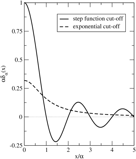
Figure 1: The form of the interaction potential Eq. (20) for step function [$\Lambda_{\alpha}(k)=\Theta(|k|-\pi/\alpha)$] and exponential [$\Lambda_{\alpha}(k)=\exp\left(-\alpha|k|\right)$] cut-offs.

The canonical transform reveals that the forward-scattering mediates attractive interactions between the $f$ electrons; as such, it can account for the observed segregation seg1D and phase separation. FGM96 ; GJL96 This is not unexpected, as the forward-scattering $c$ electrons transfer small crystal momentum ($\ll k_{F}$) to the $f$ orbitals, thus only interacting with the long-wavelength features of the underlying $f$-electron configuration.

To fully understand the physical origin of Eq. (20) we must consider the details of the bosonization process. Because of the bosonic wavelength cut-off, our treatment can only describe density fluctuations over distances $>{\cal{O}}(\alpha)$. The bosonic fields cannot distinguish separations less than this distance, hence the smeared canonical field commutators Eq. (7) and Eq. (8). Our description of this system thus assumes that the $c$ electrons are delocalized over a characteristic length $\sim\alpha$: the $\alpha$-smeared $\delta$-functions [Fig. (1)] may be very crudely conceived as the probability density profile of these delocalized electrons, i.e $|\psi(x)|^{2}\propto\delta_{\alpha}(x)$. The finite spread of the $c$-electron wavefunctions carries the interorbital Coulomb repulsion over several lattice sites [see Eq. (17)], directly leading to the segregating interaction Eq. (20).

In the familiar bosonization description of one-component systems such as the Hubbard model, making $\alpha$ arbitrarily small does not alter the critical properties of the model; in particular, we still obtain the Luttinger liquid fixed point behaviour. G:QP1D In these models $\alpha$ is regarded as a short-distance cut-off which defines the minimum length scale in the system (usually the average inter-electron separation $\sim k_{F}^{-1}$), much as the infrared cut-off in field theory. To understand the long-wavelength behaviour we need only keep $\alpha$ as a formally finite parameter. Such arguments cannot, however, be made for the $c$ electrons in the FKM, where the limiting length scale of the bosonic description is determined by the interactions with the localized $f$ electrons: the parameter $\alpha$ therefore enters our bosonic theory as a finite but undetermined length. We estimate $\alpha$ by examining the short-range fermionic scattering of the $c$ electrons off the $f$ orbitals.

As is well-known, the configuration adopted by the $f$ electrons in the FKM acts as a single-particle potential for the $c$ electrons. That is, the $c$ electrons move in a site-dependent potential that takes only two values $+G/2$ or $-G/2$, corresponding to occupied and unoccupied underlying $f$ orbitals respectively. Below the average inter-electron separation ($k_{F}^{-1}=a/\pi{n^{c}}$), the $c$ electrons move independently of one another and their motion is therefore described by a single-particle Schrödinger equation. In the limit $n^{c}\rightarrow 0$ the average inter-particle separation is much larger than the lattice constant: it is here acceptable to take the continuum limit of the lattice model, yielding a simple form for the Schrödinger equation describing the low-energy ($E=0$) wavefunctions $\psi(x)$:

$$\partial^{2}_{x}\psi(x)=Gm\langle{\tau^{z}_{x}}\rangle\psi(x)$$ (24)

here $m$ is the bare electron mass.

The motion of the $c$ electrons across the lattice is analogous to the familiar problem of elementary quantum mechanics of a particle in a finite well. Schiff For a $c$-electron moving in a region free from $f$ electrons ($\langle{\tau^{z}_{x}}\rangle=-\tfrac{1}{2}$), the energy of the $c$ electron exceeds the potential and so we find the solutions for $\psi(x)$ to be plane waves. In contrast, the $c$-electron energy is less than the potential in a region of occupied $f$ orbitals ($\langle{\tau^{z}_{x}}\rangle=\tfrac{1}{2}$): we therefore find exponentially decaying solutions $\psi(x)\sim\exp(-x/\zeta)$ characterized by the length scale $\zeta\sim\sqrt{1/G}$. Since we identify $\alpha$ with the finite spread of the delocalized $c$ electrons across the orbitals, we conclude that $\alpha\sim\zeta$. We therefore expect $\alpha=b\sqrt{t/G}$ where $b$ is a constant to be determined.

III.1.1 Relationship to the KLM

The similarity of the canonical transform Eq. (14) to that used by Honner and Gulácsi in their treatment of the KLM suggests a connection between the two models. This relationship is best revealed by considering the single-impurity limit of these lattice models; for the FKM, the associated impurity problem is the XEP.

As is well known, the sudden appearance of the core hole in the XEP excites an infinite number of electron-hole pairs in the conduction band, leading to singular features in the X-ray spectrum (the orthogonality catastrophe). Schotte and Schotte recast the problem in terms of Tomonaga bosons: the core hole potential directly couples to the boson modes of the scattering electrons, and may be removed by a suitable shifting of the oscillator frequencies. SS69 Our own canonical transform Eq. (14) repeats this procedure across the 1D lattice. Although the $f$ electrons in the FKM are static, the appearance of the core hole in the XEP is equivalent to suddenly turning on the interactions in the FKM. Since we start with non-interacting boson fields in Eq. (13), this is a perfect analogy.

The spin-$\tfrac{1}{2}$ Kondo impurity is another classic example of the orthogonality catastrophe, although the singular behaviour here arises due to the shifting of the spin-sector boson frequencies. In the usual Abelian bosonization approach the boson modes only directly couple to the $z$-component of the impurity spin: ignoring the transverse terms the problem is identical in form to the XEP. Although these transverse terms somewhat complicate the analysis, for special values of $J^{z}$ (the Toulouse point), T69 it is possible to map the problem to the exactly solvable resonant-level model by shifting the $c$-electron boson frequencies as in the XEP. S70 For the lattice case this argument may be generalized to arbitrary $J^{z}$: HG Honner and Gulácsi’s canonical transform therefore shifts the KLM’s spin-sector boson frequencies in precisely the same way as the transform Eq. (14) shifts the charge-sector boson frequencies in the FKM.

The similarity between the charge-sector physics of the FKM and the spin-sector physics of the KLM suggests a parallel between the segregating interaction Eq. (20) and the Kondo double-exchange. This is made explicit by our boson-pseudospin representation: ignoring the backscattering term in Eq. (13), the Hamiltonian is identical to the spin-sector of a forward-scattering $J_{\perp}=0$ KLM. Within their Abelian bosonization description, Honner and Gulácsi found the forward-scattering $z$-exchange term in the KLM directly responsible for mediating the double-exchange between the localized spins. HG The origin of this double-exchange term is therefore identical to our segregating interaction.

The shifting of the FKM’s charge-sector Bose frequencies produces distortions of the $c$-electron density in response to the local $f$-occupation [see Eq. (17)]. These deviations from the homogeneous noninteracting density $n^{c}_{0}$ may be interpreted as polaronic objects; SS69 note however that because of the lack of fluctuations in the $f$ orbitals, these distortions are frozen into the ground state. This illustrates an important departure from the KLM physics, where the spin-flip ($J_{\perp}$-) exchange terms cause the $z$-component of the lattice spins to fluctuate, giving the distortions of the $c$-electron spin density (i.e. spin polarons) mobility.

It is possible to modify the FKM in order to replicate this aspect of the KLM physics. The simplest such extension is an on-site hybridization term between the $c$ and $f$ orbitals, ${\cal{H}}_{\text{\tiny{hyb}}}=V\sum_{j}\{c^{\dagger}_{j}f_{j}+\mbox{H.c.}\}$: adding ${\cal{H}}_{\text{\tiny{hyb}}}$ to Eq. (1) gives the quantum Falicov-Kimball model (QFKM). Using a bosonization mapping at the Toulouse point, Schlottmann found that the $J_{\perp}$-exchange term of the Kondo impurity is equivalent to the hybridization potential in the single-impurity limit of the QFKM. Schlottmann In the lattice case, the polaronic distortions acquire mobility as in the KLM: this coupling of the $c$- and $f$-electron densities may be identified as a Toyozawa “electronic polaron”. T54 Electronic polarons in the QFKM have previously been studied by Liu and Ho; Liu&Ho our work on the 1D QFKM largely confirms their scenario. BG06 A complete account of this work is in preparation. BGinprep

III.2 The longitudinal fields

The other two terms in the transformed Hamiltonian involving the $\tau$ pseudospins are a constant and a site-dependent longitudinal field. The former is only of importance to the VTP: the renormalization of the $f$-level by the Coulomb interaction will drive a “classical” valence transition. The sign of this term is proportional to $n^{c}_{0}-\tfrac{1}{2}$, which implies a strong dependence upon the noninteracting band structure: if $\epsilon_{f}>0$, the $f$-level will be renormalized upwards, emptying its contents into the $c$-band; for $\epsilon_{f}<0$ the $f$-level is lowered below the $c$-band, and so all electrons will eventually possess $f$-electron character. Since this term does not determine the configuration adopted by the $f$ electrons but rather only their number, we leave further discussion to when we analyze the VTP phase diagram.

The site-dependent field is of more general interest. This originates from the $2k_{F}$-backscattering correction and is directly responsible for the well-known crystalline order in the FKM. Before demonstrating how the crystalline $f$-configurations can be extracted from this term, we first briefly review the present understanding of the weak-coupling periodic phases.

The origin of the crystalline order is a Peierls-like mechanism: a one-dimensional metal is always unstable towards an insulating state when in the presence of a periodic potential with wavevector $2k_{F}$. P:QTS In the context of the FKM, a Peierls instability can arise when the $f$-electrons crystallize in a periodic configuration with wavevector $2k_{F}$. This is the case for weak coupling and we repeat a theorem due to Freericks and Falicov: FF90 given rational $c$-electron density $n^{c}=p/q$ ($p$ prime with respect to $q$) and $G/t\ll{q}$, then for $f$-electron density $n^{f}=p^{f}/q$ ($p^{f}$ not necessarily prime with respect to $q$) the $f$ electrons occupy the sites $x=nq+k_{j}$ where $n$ is an arbitrary integer and the $k_{j}$ satisfy the relation

$$(pk_{j})\bmod{q}=j,\quad j=0,1,\ldots,p^{f}-1$$ (25)

For example, consider the case $n^{c}=\frac{3}{8}$ and $n^{f}=\frac{5}{8}$. The unit cell has eight sites, and the $f$ electrons occupy the first, second, fourth, fifth and seventh sites [see Fig. (2)(a)].

Our approach reproduces this important result. In the pure crystalline phase, the $c$-electron spectrum is gapped. F03 We therefore replace $\phi(x_{j})$ in the cosine term of Eq. (18) by the uniform average $\langle{\phi}\rangle$. Ignoring the ${\cal{O}}(G^{2})$ Ising interaction, at weak coupling the $\tau$ pseudospins are therefore arranged by the field

$$\frac{2GAa}{\alpha}\sum_{j}\tau^{z}_{j}\cos\left(2[\langle{\phi}\rangle+{\cal{K}}(j)-k_{F}{x_{j}}]\right)$$ (26)

The string operator ${\cal{K}}(j)$ is a constant of the motion and so it may be replaced by its eigenvalue. Referring to Eq. (19), this term subtracts the magnetization of the $\tau$ pseudospins more than $\alpha$ to the right of site $j$ from the magnetization of the $\tau$ pseudospins more than $\alpha$ to the left of site $j$: for an infinite chain in the pure crystalline phase this quantity vanishes, ${\cal{K}}(j)=0$. The value of $\langle{\phi}\rangle$ must be chosen to minimize the backscattering energy. This of course implies a non-trivial dependence upon the $f$-electron concentration: for a $Q$-site unit cell with $f$-electron concentration $q^{f}/Q$, we must minimize $\langle\phi\rangle$ over the sum

$$\sum_{l=1,q^{f}}\lambda_{l}-\sum_{l=q^{f}+1,Q}\lambda_{l}$$ (27)

where $\lambda_{l}=\cos\{2[\langle{\phi}\rangle-k_{F}{x_{l}}]\}$ and $l$ is chosen such that $\lambda_{1}\leq\lambda_{2}\leq\ldots\leq\lambda_{Q}$, $x_{l}$ lying within the unit cell. This minimization is most easily accomplished numerically; $\langle\phi\rangle$ is restricted to values in the interval $[0,\pi)$.

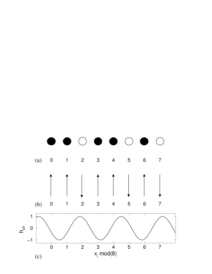
Figure 2: (a) The configuration of the $f$-ions in the weak-coupling homogeneous unit cell for $n^{c}=\frac{3}{8}$, $n^{f}=\frac{5}{8}$. The filled and empty circles represent occupied and unoccupied sites respectively. (b) The pseudospin representation for the configuration (a). (c) The variation of the effective magnetic field $h_{\text{\tiny{eff}}}$ produced by the $2k_{F}$-backscattering correction across the unit cell. $h_{\text{\tiny{eff}}}$ is in units of $2GAa/\alpha$.

The sum Eq. (27) assumes that the $q^{f}$ $f$ electrons per unit cell will occupy the $q^{f}$ lowest-energy sites in the potential Eq. (26). In terms of the pseudospins, there is a fixed magnetization $q^{f}/Q-\frac{1}{2}$ per unit cell; the $\uparrow$-spins occupy the sites with the smallest magnetic field, with the $\downarrow$-spins sitting on the remaining $Q-q^{f}$ sites. For the example above with $n^{c}=\frac{3}{8}$ and $n^{f}=\frac{5}{8}$, we find $\langle\phi\rangle\approx 0.589$ and so the $f$ electrons experience a potential

$$\frac{2GAa}{\alpha}\sum_{j}\tau^{z}_{j}\cos\left(1.178-\frac{3\pi{x_{j}}}{4a}\right)$$

We plot this potential in Fig. (2)(c) along with the $\tau$ pseudospin orientations [Fig. (2)(b)]. It is in good agreement with the exact result Eq. (25), although there is some ambiguity with respect the position of the $f$-electron at the fifth and sixth sites. Closer correspondence may be achieved by taking into account higher-order backscattering processes; because bosonization is fundamentally a long-wavelength method, this approach does not replace the exact calculations. Nevertheless, our analysis convincingly demonstrates that bosonization is capable of describing crystallization of the $f$ electrons in the FKM.

Before proceeding to a discussion of the FKM’s phase diagram, we note that as the number of $f$ electrons is limited in the FKM, it may not be possible for a pure crystalline phase to gap the $c$-electron spectrum at the Fermi energy. In particular, for irrational $c$-electron filling the field Eq. (26) will be incommensurate with the lattice. Although this situation remains unclear, in the related case of rational $c$-electron filling $n^{c}=p/q$ and $f$-electron filling $p^{\prime}/q<n^{f}<(p^{\prime}+1)/q$ the system phase separates into regions with periodic phases determined by Eq. (25) for $p^{f}=p^{\prime}$ and $p^{f}=p^{\prime}+1$. FGM96 It is also known that for $f$-electron concentrations $n^{f}\lesssim 0.371$ and $n^{f}\gtrsim 0.629$ the system exists in a mixture of a crystalline phase and a homogeneous phase (the empty or full configuration). This phase separation behaviour cannot be explained purely in terms of $c$-electron backscattering.

IV The Effective Hamiltonian

By themselves, the Ising interaction [Eq. (20)] and the longitudinal field [Eq. (26)] explain the SEG and crystalline phases respectively. To understand the origin of the phase separation or interpret the numerically-determined phase diagram, however, we must consider the interplay of these terms. In particular, it is desirable to have a simple effective Hamiltonian for the $f$ electrons that includes both the crystallizing and segregating tendencies of the FKM.

The transformed Hamiltonian Eq. (18) offers a straight-forward route to such a description of the $f$-electrons. With the removal of the term describing the forward-scattering interaction, the only coupling between the two species is in the $2k_{F}$-backscattering correction. In the weak-coupling crystalline phases it is possible to completely decouple the $f$ electrons from the $c$ electrons by replacing the bosonic $\phi(x_{j})$ field by its expectation value. Combining Eq. (26) with the interaction Eq. (20), we obtain an effective spin-$\tfrac{1}{2}$ Ising model for the $f$ electrons valid throughout the region where the crystalline phases are realized:

$${\cal{H}}_{\text{\tiny{eff}}}=-\frac{G^{2}a^{2}}{2\pi v_{F}}\sum_{j,j^{\prime}}\tau^{z}_{j}\delta_{\alpha}(x_{j}-x_{j^{\prime}})\tau^{z}_{j^{\prime}}+\frac{2GAa}{\alpha}\sum_{j}\tau^{z}_{j}\cos\left(2[\langle{\phi}\rangle+{\cal{K}}(j)-k_{F}{x_{j}}]\right)$$ (28)

This is an important result, but our approach is not limited only to the crystalline phases: for other configurations, the form of the effective Hamiltonian Eq. (28) remains valid, although the site-dependence of the longitudinal field is different. In the crystalline phases ${\cal{K}}(j)$ is vanishing; in the segregated or phase separated states, however, ${\cal{K}}(j)$ has linear variation. Ignoring the short-range deviation of $\text{sgn}_{\alpha}(x_{j})$ from the true sign-function, we write

$${\cal{K}}(j)\approx\frac{Ga}{v_{F}}\sum_{n=1}\left(\tau^{z}_{j+n}-\tau^{z}_{j-n}\right)$$ (29)

Assume a phase separation between phase $A$ and phase $B$ with the boundary at $j=0$. Then for $j^{\prime}\gg{1}$ we have approximately G04

$${\cal{K}}(j^{\prime})\approx{\cal{K}}(0)+\frac{Ga}{v_{F}}\left(\langle\tau^{z}\rangle_{A}-\langle\tau^{z}\rangle_{B}\right)|j^{\prime}|$$ (30)

where the subscripts $A$ and $B$ refer to the magnetization in the $A$ and $B$ phases respectively. We have chosen the sign of the linear term by choosing phase $A$ to be realized to the right and phase $B$ to the left of $j=0$. Note that ${\cal{K}}(j)$ is constant for a pure phase, as we expect.

For the SEG phase, the division of the lattice into empty and full sections implies a variation ${\cal{K}}(j)\sim{(Ga/2v_{F})|j|}$. Although the conduction electron spectrum does not display a gap, the decoupling procedure for the field $\phi(x_{j})$ used in Sec. III.2 may be easily generalized. In the SEG phase, the conduction electrons are restricted to a fraction $(1-n^{f})$ of the lattice, where they behave as a non-interacting electron gas. We therefore replace $\phi$ in Eq. (26) by its non-interacting average $\langle{\phi}\rangle=0$ to obtain the effective pseudospin Hamiltonian in the SEG phase.

The phase-separation between the crystalline and empty phase is the most complex situation to analyze, as we must account for the very different behaviour of the $c$-electrons for the two configurations. Exact diagonalization calculations on 3200 site chains reveal that the momentum distribution of the $c$-electrons is essentially a superposition of the gapped and noninteracting forms corresponding to the crystalline and empty regions of the lattice, with vanishingly small correction due to the interface of these phases in the thermodynamic limit $N\rightarrow\infty$. F03 Decoupling the $c$-electron fields as above, we take different averages of the $\phi$-field in the bulk of the two phases: for the empty phase, we use the noninteracting value $\langle\phi\rangle=0$ while we determine $\langle\phi\rangle$ for the crystalline phase as in Sec. III.2. Approximating ${\cal{K}}(j)$ as in Eq. (30), we have ${\cal{K}}(j)\sim{(Ga/2v_{F})m|j|}$ where $m=\langle\tau^{z}\rangle_{P}+\tfrac{1}{2}$ ($\langle\tau^{z}\rangle_{P}$ is the magnetization of the periodic phase).

The effective Hamiltonian across the phase diagram is ferromagnetic Ising model in a oscillatory longitudinal field. This model exhibits all the most important aspects of FKM physics. It is, however, important to add here a cautionary note about the limitations of Eq. (28). Bosonization is an inherently long-wavelength method, and so it is therefore unreasonable to expect ${\cal{H}}_{\text{\tiny{eff}}}$ to precisely reproduce the microscopic details of the $f$-electron configuration realized for given $G$, $n^{c}$ and $n^{f}$. Rather, ${\cal{H}}_{\text{\tiny{eff}}}$ is primarily relevant to the long-wavelength physics, with the site-dependent longitudinal field acting as an essentially approximate account of the short-range crystallizing interactions. Furthermore, the form of ${\cal{H}}_{\text{\tiny{eff}}}$ is rigorously quantitatively valid only for $G\lesssim{t}$. Nevertheless, we expect that ${\cal{H}}_{\text{\tiny{eff}}}$ is at least qualitatively correct over a much larger region of the phase diagram. G04

V The ground state phase diagram

V.1 The crystallization problem

In the CP, the concentration of the $f$-electrons is fixed: the problem of the ground state phase diagram is then reduced to finding the pseudospin configuration with magnetization $n^{f}-\tfrac{1}{2}$ that minimizes the energy $\langle{{\cal{H}}_{\text{\tiny{eff}}}}\rangle$. This lattice-gas problem, although conceptually simple, does not have a general solution. It is therefore appropriate to use approximate methods to understand the physics.

In general, the segregating Ising interaction has a range $\alpha$ that extends over several lattice sites. To understand the segregation, however, we need consider only the nearest-neighbour value of the potential $\delta_{\alpha}(a)$. That is, we write the Ising interaction

$$-\frac{G^{2}a^{2}}{2\pi v_{F}}\sum_{j,j^{\prime}}\tau^{z}_{j}\delta_{\alpha}(x_{j}-x_{j^{\prime}})\tau^{z}_{j^{\prime}}\approx-\frac{G^{2}a^{2}}{\pi v_{F}}\delta_{\alpha}(a)\sum_{j}\tau^{z}_{j}\tau^{z}_{j+1}$$ (31)

This is justified as for realistic cut-off $\Lambda_{\alpha}(k)$ the interaction potential $\delta_{\alpha}(x)$ is attractive for $x<{\alpha}$ but falls off very quickly with distance [see Fig. (1)]. Truncating the interaction should not significantly alter the critical properties of the model, while considerably simplifying the analysis.

The weak-coupling phase separation into the empty and a periodic configuration requires us to extend the Ising interaction beyond the nearest-neighbour approximation used above. The restriction to fixed magnetization makes this a challenging problem to analyze and a general criteria for the phase separation is beyond the capabilities of our approach. We shall nevertheless demonstrate the origin of the phase separation for a single set of input parameters, noting the importance of considering a delocalization length $\alpha>2a$.

V.1.1 Segregation

In the pseudospin “language” of the effective Ising model Eq. (28), the SEG phase corresponds to a ferromagnetic state with two domains: a single block of $\uparrow$-spins occupying a fraction $n^{f}$ of the lattice and $\downarrow$-spins in the remaining $(1-n^{f})N$ sites. From the form of ${\cal{H}}_{\text{\tiny{eff}}}$, we see that the critical Coulomb repulsion $G_{c}$ for the onset of segregation is related to the critical ratio $J/h$ for the onset of ferromagnetism in the model

$${\cal{H}}_{\text{\tiny{}}}=-J\sum_{j}\tau^{z}_{j}\tau^{z}_{j+1}+h\sum_{j}\tau^{z}_{j}\cos(\omega_{j}{j}+\phi_{j})$$ (32)

where $\omega_{j}$ and $\phi_{j}$ take different constant values in different macroscopic regions of the lattice.

The Ising model Eq. (32) has been studied for constant $\omega$ and $\phi$ by Sire S93 . For $\omega/\pi$ irrational, i.e. the quasiperiodic Ising Model (QPIM), it is found that the critical Ising coupling has the form $J_{c}=h/\sin(\tfrac{1}{2}{\omega})$. At couplings $J>J_{c}$ the ground state is ferromagnetically ordered; the adiabatic phase (where the spins align antiparallel to the direction of the longitudinal field $h^{z}_{j}$) is however only realized for $J<J_{c2}<J_{c}$ where $J_{c2}=h\sin(\tfrac{1}{2}\eta\omega)\sin(\tfrac{1}{2}[\eta+1]\omega)/\sin(\tfrac{1}{2}\omega)$ and $\eta$ is the largest integer smaller than $\pi/\omega$. For the intermediate couplings $J_{c}>J>J_{c2}$ the ground state is a “mixture” of the adiabatic and ferromagnetic phases. This “mixed” state consists of a quasiperiodic arrangement of clusters of adiabatically- and ferromagnetically-ordered spins. These clusters form as neither the Ising interaction nor the magnetic field are strong enough to order the entire lattice: ferromagnetic clusters occur where the magnetic field is weak compared to the Ising term, while paramagnetic clusters are found where the Ising term is weak compared to the magnetic field. Note that this is not a phase separation phenomenon.

The work on the QPIM in LABEL:S93 was performed within the grand canonical ensemble and so we must be cautious in relating these results to the effective Hamiltonian Eq. (28). The expression for the critical Ising coupling $J_{c}$ was deduced from general arguments that should remain valid at fixed magnetization. Indeed, the difference in energy per site between the single-domain and the two-domain (SEG) solution vanishes as ${\cal{O}}(N^{-1})$ in the thermodynamic limit. The QPIM results should therefore correctly capture the competition between the adiabatic and ferromagnetic orders present in Eq. (28): this provides a condition for segregation to dominate crystallization. Although the QPIM at weak- and strong-coupling corresponds to the behaviour seen in the small- and large-$G$ FKM, the agreement breaks down at intermediate coupling. This is due to the use of the grand canonical ensemble in LABEL:S93, as phase separation cannot occur in the FKM without fixed electron concentration GUJ94 .

We note that the effective Ising Hamiltonian derived for the SEG phase must always display ferromagnetic order. That is, within its range of applicability, the Ising interaction always dominates the magnetic field. Although the SEG effective Hamiltonian might display adiabatic order at weak coupling, since crystallization in the FKM occurs in this limit a different form of the longitudinal field must be used in Eq. (28). To use the QPIM condition to determine the boundary of the SEG phase, we therefore assume that the range of applicability of the SEG effective Hamiltonian corresponds exactly to the extent of ferromagnetic order.

A further difficulty encountered when applying the FM condition derived for the QPIM is that the frequency of the magnetic field in the SEG phase takes two values $\omega_{\pm}\approx{2(\pi{n^{c}}\pm{Ga/2v_{F}})}$ for each bulk phase (i.e. the empty and full sections of the lattice). Although it is not possible to determine which value is realized for which section, the FM condition also holds for half-spaces and so we choose $\omega_{+}$ which gives the observed monotonic dependence of the critical line on the filling for weak- and intermediate-coupling GJL96 . Since bosonization is quantitatively correct in the weak-coupling limit, the expressions for $\omega_{+}$ will only rigorously hold for $G$ small as compared to the conduction electron bandwidth. In this limit segregation occurs for $n^{c}\rightarrow 0$ and so $\omega_{+}\approx{Ga/v_{F}}$; we use this form to determine the weak-coupling critical line.

Comparing the coefficients in Eq. (28) with those in Eq. (32) we find after some algebra the condition for segregation

$$\lim_{n^{c}\rightarrow 0}\frac{G_{c}a}{v_{F}}\sin(\omega_{+}/2)=\frac{G_{c}a}{v_{F}}\sin({G_{c}a}/{2v_{F}})=\frac{2A\pi}{\alpha\delta_{\alpha}(a)}$$ (33)

We immediately deduce an important feature of the phase diagram: from general principles we know that $\alpha\gtrsim{\cal{O}}(k_{F}^{-1})$ as $n^{c}\rightarrow 0$. Since $\delta_{\alpha}(a)\sim{\alpha^{-1}}$ for $\alpha\gg{a}$, the denominator of the RHS of Eq. (33) tends to a constant as $\alpha\rightarrow\infty$. For the expression to be consistent, we hence require $G_{c}a/v_{F}=\mbox{constant}>0$ as $n^{c}\rightarrow 0$: we recover the result that segregation occurs at arbitrarily small $G$ in the limit of vanishing conduction electron concentration KL86 .

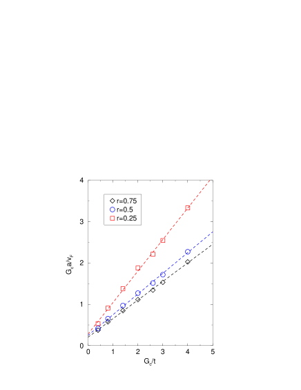
Figure 3: (color online) Dependence of $G_{c}a/v_{F}$ on $G_{c}/t$ for three values of the ratio $r$. The data is taken from LABEL:GJL96.

For finite filling, we can use our estimate for $\alpha/a\sim{\sqrt{t/G}}$ to obtain the critical line $G_{c}$ at weak- to intermediate-coupling. Assuming $G_{c}a/v_{F}\ll{\pi/2}$ for small $G_{c}$, we linearize the sine function in Eq. (33); after some algebra we find

$$G_{c}=4t\sin(\pi{n^{c}})\sqrt{\frac{A\pi}{\alpha\delta_{\alpha}(a)}}$$ (34)

At weak coupling, we have $\alpha\gg{a}$: Taylor-expanding the RHS of Eq. (34) in powers of $a/\alpha$, we keep terms up to second order. The coefficients in this expansion are dependent upon the form of $\Lambda_{\alpha}(k)$ used; for exponential cut-off we have

$$G_{c}a/v_{F}\approx\sqrt{4A\pi^{2}}\left(1+\frac{a^{2}}{2\alpha^{2}}\right)$$ (35)

Substituting our estimate for $\alpha$ into this equation, we thus expect a linear relationship between $G_{c}a/v_{F}$ and $G_{c}$. This also holds at intermediate couplings, as clearly verified by the numerical results of LABEL:GJL96: we plot $G_{c}a/v_{F}$ as a function of $G_{c}$ in Fig. (3) for three values of the fraction of electrons in the $c$-band $r=n^{c}/n=0.75$, $0.5$ and $0.25$. After some re-arrangement of Eq. (35), we obtain the general form of the critical line

$$G_{c}(r,n)=\frac{2B(r)\sin(\pi{rn})}{1-2C(r)\sin(\pi{rn})}$$ (36)

The numerical constants $B(r)$ and $C(r)$ are the $y$-intercept and gradient of the lines in Fig. (3) respectively; they are related to the fitting parameters in Eq. (33) by $A={B(r)}^{2}/4\pi^{2}$ and $\alpha/a=\sqrt{B(r)t/2C(r)G_{c}}$.

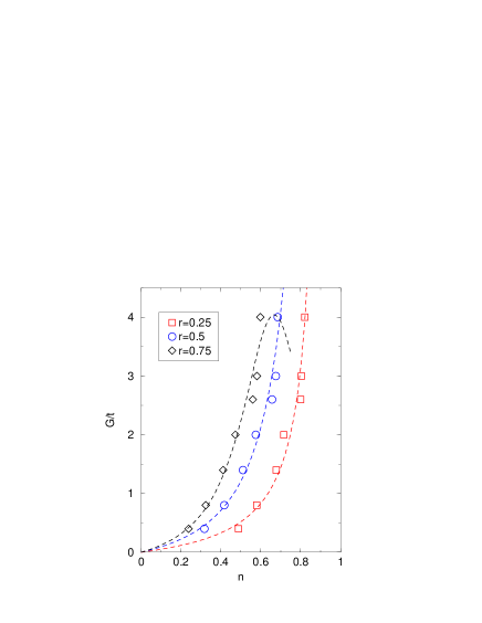
Figure 4: (color online) Dependence of $G_{c}/t$ on $n$ for three values of the ratio $r$. The data is taken from LABEL:GJL96. The critical lines $G_{c}(n)$ of best fit are as derived from Fig. (3). For each value of $r$, the SEG phase occurs for $G>G_{c}(n)$.

From our fit to the lines in Fig. (3) we find the critical lines for the three values of $r$

$$G_{c}(n)/t=\begin{cases}\vspace{0.25cm}\displaystyle{\frac{0.5666\sin(n\pi/4)}{1-1.5212\sin(n\pi/4)}}&r=0.25\\ \vspace{0.25cm}\hskip 14.22636pt\displaystyle{\frac{0.5\sin(n\pi/2)}{1-\sin(n\pi/2)}}&r=0.5\\ \displaystyle{\frac{0.4112\sin(3n\pi/4)}{1-0.8982\sin(3n\pi/4)}}&r=0.75\end{cases}$$ (37)

These three curves, along with the numerical data, are plotted in Fig. (4). The curves track the data very well for both $r=0.25$ and $r=0.5$; for $r=0.75$, however, there is a significant divergence between Eq. (37) and the numerical results as the coupling increases. The curve Eq. (37) has a maximum at $n=2/3$ (i.e. $n^{c}_{0}=1/2$), but no evidence of this maximum is found in the weak-coupling numerical results. Rather, we expect the critical line to continue to diverge as half-filling is approached. We thus conclude that there is a change in the form of $G_{c}(n)$ at intermediate-coupling. The numerical analysis of Gruber et al. indicates that this occurs at approximately $G\approx 2.5t$ GUJ94 , which is consistent with the observed deviation from the weak-coupling critical line in Fig. (4).

Any deviation from the weak-coupling form Eq. (36) for $r=0.25$ and $r=0.5$ is much less obvious. Since the $G\rightarrow\infty$ asymptotic form of $G_{c}(r,n)$ stated in LABEL:GUJ94 is not the same as that given by Eq. (37), we do however expect that a different expression is valid at $G\gg{t}$. A new functional dependence on $n$ in the strong-coupling regime is reasonable and does not contradict our own analysis: we have emphasized that bosonization is only quantitatively accurate for weak-coupling. Importantly, the physical processes driving the segregation will remain invariant across the phase diagram.

V.1.2 Phase separation

At weak-coupling and sufficiently small or large $f$-electron concentration, the FKM is unstable towards a phase separation between a homogeneous and a crystalline configuration. FGM96 Unlike the SEG phase, it is necessary to consider the range of the forward-scattering Ising interaction as extending beyond the nearest neighbour to observe these phases.

To illustrate the importance of these long-range terms, we examine the weak-coupling limit of Eq. (28) for the case $n^{c}=\tfrac{1}{2}$, $n^{f}=\frac{1}{4}$. Of the Ising interaction Eq. (20) we keep the nearest-neighbour ${\cal{J}}_{1}$ and next-nearest neighbour ${\cal{J}}_{2}$ terms. For $G\ll{t}$, we discard ${\cal{K}}(j)$ in the cosine’s argument, leaving a staggered-field variation. We thus find an effective Hamiltonian of the form

$${\cal{H}}_{\text{\tiny{}}}=-{\cal{J}}_{1}\sum_{j}\tau^{z}_{j}\tau^{z}_{j+1}-{\cal{J}}_{2}\sum_{j}\tau^{z}_{j}\tau^{z}_{j+2}-h\sum_{j}(-1)^{j}\tau^{z}_{j}$$ (38)

We calculate $E=\langle{{\cal{H}}_{\text{\tiny{}}}}\rangle$ for three situations: (a) the most homogeneous phase with period-$4$ pseudospin unit cell $[\uparrow\downarrow\downarrow\downarrow]$; (b) phase separation between the empty phase ($[\downarrow]$) and the period-$2$ phase with unit cell $[\uparrow\downarrow]$; and (c) segregation. We find the energy per site for each of these configurations

$$E/N=\begin{cases}-\tfrac{1}{4}{h}&\text{config. (a)}\\ -\tfrac{1}{2}{\cal{J}}_{2}-\tfrac{1}{4}{h}&\text{config. (b)}\\ -\tfrac{1}{2}{\cal{J}}_{1}-\tfrac{1}{2}{\cal{J}}_{2}&\mbox{config. (c)}\end{cases}$$ (39)

These expressions hold in the thermodynamic limit $N\rightarrow\infty$.

We see that even an arbitrarily small ${\cal{J}}_{2}$ destabilizes configuration (a) toward phase separation. Since at weak-coupling we expect ${\cal{J}}_{1}\ll{h}$, segregation will however not occur; instead configuration (b) is the most stable. This is the weak-coupling phase separation between a crystalline and the empty phase found by Freericks et al. FGM96 Although our analysis does not provide a general condition for this peculiar form of phase separation to occur, it shows that the physical origin of this effect is the competition between segregation and crystallization. We also see how fixed $c$- and $f$-electron populations are essential for the appearance of this phenomenon.

The phase separation between periodic and uniform states in the $n<1$ FKM is not confined to the weak-coupling limit of the phase diagram, but is also present at intermediate- and strong-coupling. FB93 ; GJL96 For $G>t$ our bosonization approach will at least qualitatively capture the physics of the FKM: we therefore expect that the competition between segregation and crystallization that we have identified as the origin of the weak-coupling phase separation will also be responsible for these intermediate- and strong-coupling phases.

V.2 The valence transition problem

In contrast to the CP, the VTP has received little attention in the FKM literature, despite the two interpretations being very closely related. In both the CP and the VTP the $f$-orbital occupation is a good quantum number, and the ground state may be defined as the configuration of the $f$ electrons that minimizes the energy of the $c$ electrons. The only difference between the CP and the VTP is that in the former the distribution of the electrons across the orbitals is fixed, while in the latter the interactions determine the equilibrium populations.

For given interacting equilibrium populations in the VTP, the configuration adopted by the $f$-electrons should be the same as in the CP for the same fixed electron populations. As discussed in Sec. III.2, the first two terms of Eq. (18) determine the equilibrium distribution of the electrons across the $c$ and $f$ orbitals. They can be identified as the noninteracting $c$-electron Hamiltonian and the $f$-level shift due to the Coulomb repulsion. To estimate the electron distribution for finite $G$ we therefore assume that the distribution of the $nN$ electrons across the two orbitals in the FKM is the same as in the system

$${\cal{H}}=-t\sum_{j}\left\{c^{\dagger}_{j}c_{j+1}+\mbox{H.c.}\right\}+[\epsilon_{f}+G(n^{c}_{0}-\tfrac{1}{2})]\sum_{j}n^{f}_{j}$$ (40)

That is, the contribution of the ordering terms in Eq. (18) to the shift in electron density between the $c$ and $f$ orbitals is taken to be negligible. This can be easily justified for a thermodynamically large system: the difference between the energy per site of the SEG phase and the empty or full phases due to the Ising interaction is of order $1/N$; and the average value of the bacscattering longitudinal field across the lattice is vanishing.

We find that for noninteracting $c$-electron population $n^{c}_{0}$ (fixed by the band structure) the $c$-electron population in the interacting system is given by

$$n^{c}=\frac{1}{\pi}\arccos\left(\cos(n^{c}_{0}\pi)-\frac{G}{4t}(2n^{c}_{0}-1)\right)$$ (41)

In LABEL:GJL96 phase diagrams for the CP in the $n^{c}$-$n^{f}$ plane at constant $G$ are presented For each $G$ the boundary between the SEG phase and the crystalline or phase separated states is given by a straight line of the form ${n^{c}}=\gamma(1-n^{f})$ where $\gamma$ is a constant determined from the numerical phase diagrams. Using the fixed electron concentration condition we may re-write this

$$n^{c}=\frac{\gamma}{1-\gamma}(1-n)$$ (42)

where $n=n^{c}+n^{f}$ is the total electron concentration. Equating the RHS of Eq. (41) and Eq. (42) we obtain the equation

$$\cos\left(r_{0}n\pi\right)-\frac{G}{4t}\left(2r_{0}n-1\right)-\cos\left(\frac{\pi\gamma}{1-\gamma}[1-n]\right)=0$$ (43)

where $r_{0}=n^{c}_{0}/n$ is the fraction of $c$-electrons in the non-interacting system. For given $r_{0}$ and $G$, the value of $n$ that solves Eq. (43) gives the maximum filling for which the SEG phase is stable.

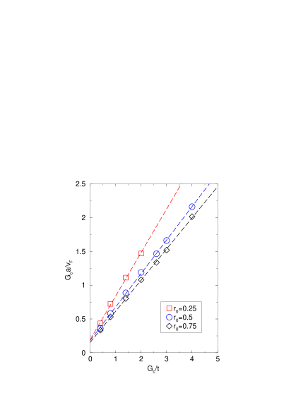
Figure 5: (color online) Dependence of $G_{c}a/v_{F}$ on $G_{c}/t$ for three values of the ratio $r_{0}$ in the VTP. The data is taken from LABEL:GJL96.

Using this procedure we calculate from the results of LABEL:GJL96 the critical value of $n$ for $r_{0}=0.25$, $0.5$ and $0.75$. Proceeding with our analysis as in the CP (Sec. V.1.1) we find that the linear relationship between $G_{c}a/v_{F}$ and $G_{c}$ is also well obeyed in the VTP [Fig. (5)]. As such, at weak-coupling the critical line $G_{c}(r_{0},n)$ has the form given by Eq. (36). In particular, we find from the linear best fit to the data in Fig. (5) the following expressions

$$G_{c}(n)/t=\begin{cases}\vspace{2.5mm}\displaystyle{\frac{0.389\sin(n\pi/4)}{1-1.289\sin(n\pi/4)}}&r_{0}=0.25\\ \vspace{2.5mm}\displaystyle{\frac{0.363\sin(n\pi/2)}{1-0.992\sin(n\pi/2)}}&r_{0}=0.5\\ \displaystyle{\frac{0.307\sin(3n\pi/4)}{1-0.923\sin(3n\pi/4)}}&r_{0}=0.75\end{cases}$$ (44)

These are illustrated in Fig. (6) along with the critical lines for the associated $r=r_{0}$ CP [Eq. (37)]. As before, we find excellent agreement between the data points and the fitted curves for both $r_{0}=0.5$ and $r_{0}=0.25$. Again, however, we find for $r_{0}=0.25$ a significant divergence between the curve Eq. (44) and the data for higher values of $G$. The origin of this discrepancy is presumably the same as in the CP. Note also that only four numerical values are presented for $r_{0}=0.25$: for $G\gtrsim 3t$ the segregated configuration is realized for all $n<1$. This is not unexpected, as in this case we have the smallest $n^{c}_{0}$, and thus largest shifting of the $f$-level, for given $n$.

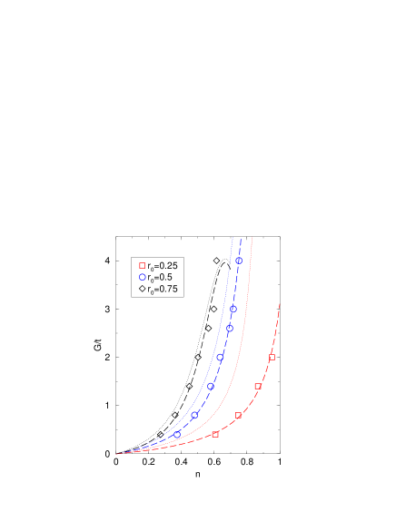
Figure 6: (color online) Dependence of $G_{c}/t$ on $n$ for three values of the ratio $r$ for the VTP. The data is taken from LABEL:GJL96. The critical lines $G_{c}(n)$ of best fit (thick dashed lines) are as derived from Fig. (5). For each value of $r_{0}$, the SEG phase occurs for $G>G_{c}(n)$. The thin dotted lines are the critical lines in the $r=r_{0}$ CP.

As illustrated in Fig. (4), the division of electrons between the two orbitals in the CP strongly affects the position of the critical line for segregation: the more $f$ electrons relative to $c$ electrons, the smaller the value of $G$ required to cause segregation. For $n^{c}_{0}<\tfrac{1}{2}$, turning on the interaction in the VTP will shift the $f$-level to a lower energy relative to the $c$-electron band, thus causing a transfer of electrons from the $c$ to the $f$ orbitals. Accordingly, we find that segregation in the VTP occurs at a lower value of $G$ than in the $r=r_{0}$ CP [Fig. (6)]. Eventually, the $f$-level will be shifted below the bottom of the $c$-electron band; this is the case for couplings

$$G_{\text{\tiny{full}}}\geq\frac{-4t[1-\cos(r_{0}n\pi)]}{2n^{c}_{0}-1}$$ (45)

The absence of any $c$ electrons to cause crystallization or segregation means that any $f$-electron configuration is the ground state. For $r_{0}=0.25$ and $n=1$ the critical coupling $G_{\text{\tiny{full}}}\approx 2.34t$, explaining the absence of any $G>2t$ data.

Conversely, for $\epsilon_{f}>0$ and hence $n^{c}_{0}>\tfrac{1}{2}$, turning on the interaction will shift the $f$-level to higher energies and empty the $f$-electron orbitals. Segregation may not occur in this case at all, and the large-$G$ configuration is the empty phase. From our analysis, we estimate that this will be realized for

$$G_{\text{\tiny{empty}}}\geq\frac{-4t[\cos(n\pi)-\cos(r_{0}n\pi)]}{2n^{c}_{0}-1}$$ (46)

Note that we assume $n>\tfrac{1}{2}$. This scenario is strongly supported by Farkašovský’s numerical study of the $n=1$ VTP. F95a In his $\epsilon_{f}$-$G$ phase diagram, he found that for $\epsilon_{f}>0$ ($n^{c}_{0}>\tfrac{1}{2}$) all electrons occupy the $c$-orbital states for sufficiently large $G$, while for $\epsilon_{f}<0$ ($n^{c}_{0}<\tfrac{1}{2}$) the $f$ orbitals become fully occupied as $G$ is increased.

We note in concluding that we have not addressed the case where the $f$-level does not lie at the Fermi energy in the noninteracting system. For example, for $\epsilon_{f}=0$ and $n<\tfrac{1}{2}$ the $f$-level will lie a finite energy above $e_{F}=-2t\cos(n\pi)$. On the basis of our analysis, it appears that a non-zero $f$-population will eventually appear as the $f$-level is shifted in the presence of a finite $G$. As $G$ is further increased, the $c$-electron band is eventually emptied into the $f$-level. Turning on the interactions, we thus evolve from a state without any $f$ electrons into a state with all electrons in the $f$ orbitals. We must regard this result with caution: since bosonization is an effective field theory for the excitations about the Fermi energy, it is difficult to include the localized electrons whenever $\epsilon_{f}\neq e_{F}$. In particular, the bosonic wavelength limit $\alpha$ implies an effective bandwidth cut-off for the excitations about $e_{F}$. What happens when $\epsilon_{f}$ lies outside of this effective bandwidth is unclear and we must go beyond the framework of bosonization to understand this situation. For this reason, from the point of view of bosonization the VTP is a more challenging problem than the CP.

VI Extensions of the FKM

The FKM is often studied in a modified form with the addition of extra terms to the basic Hamiltonian Eq. (1). The most common extensions are $c$-$f$ hybridization, LRP81 ; Vfinite ; Liu&Ho ; BG06 ; BGinprep $f$-electron hopping crystaltff ; Batista or the introduction of spin. DMFT ; F99 ; spin In the first two cases, the extension has a dramatic effect upon the physics: the occupation of each localized orbital is no longer a good quantum number. The CP and VTP results are applicable only as limiting behaviour and we cannot easily incorporate these additional terms into the analysis presented above. As such, below we will briefly consider several extensions that maintain the “classical” nature of the $f$ electrons: intraorbital nearest-neighbour interactions and the addition of spin. Our bosonization formalism is very well suited to assessing the impact of these extensions upon the ground states of the “bare” FKM.

VI.1 Nearest-neighbour interactions

Our study of nearest-neighbour interactions is confined to their effect upon the CP results. The same conclusions also hold for the VTP so long as the densities are normal-ordered.

VI.1.1 $c$ electrons

We write the nearest-neighbour interaction between the $c$ electrons

$${\cal{H}}_{cc}=V_{c}\sum_{j}n^{c}_{j}n^{c}_{j+1}$$ (47)

It is sufficient here to examine only the forward-scattering contributions of this interaction as the Umklapp and backscattering contributions are only relevant at half-filling G:QP1D . Since we are only interested in the effect of ${\cal{H}}_{cc}$ on the long-wavelength physics of the FKM, we may apply the continuum-limit approximation and absorb the interaction into a free-Boson Hamiltonian

$$\widetilde{{\cal{H}}}_{0}=\frac{v{a}}{2\pi}\sum_{j}\left\{\left(\partial_{x}\widetilde{\phi}(x_{j})\right)^{2}+\left(\partial_{x}\widetilde{\theta}(x_{j})\right)^{2}\right\}$$ (48)

The new Bose fields are related to the $V_{c}=0$ fields by the relations

$$\widetilde{\phi}(x_{j})=\frac{1}{\sqrt{K}}\phi(x_{j}), \widetilde{\theta}(x_{j})={\sqrt{K}}\theta(x_{j})$$ (49)

$$v = \frac{v_{F}}{K}$$ (50)

where

$$K=\frac{1}{\sqrt{1+2V_{c}v_{F}/(\pi{at^{2}})}}$$ (51)

The details of this rescaling procedure are identical to the argument for the forward-scattering sector of the XXZ chain LP75 . Note that for an attractive interaction $V_{c}=-\pi{a}t^{2}/v_{F}$ the velocity of the Boson modes vanishes: this indicates the break-down of the bosonization method, as the Luttinger liquid is unstable towards the clustering of the $c$-electrons. We may expect the SEG phase to be realized whenever this condition holds.

The bosonized FKM with the interaction Eq. (47) is identical in appearance to the $V_{c}=0$ bosonized Hamiltonian [Eq. (13)]: the first term in Eq. (13) is however replaced by Eq. (48) and the Bose fields in the other terms are replaced by their scaled forms Eq. (49). Our analysis of ${\cal{H}}_{\text{\tiny{FKM}}}+{\cal{H}}_{cc}$ also proceeds in a similar way to that in Sec. III, although we rotate the Hilbert space using a different canonical transform

$$\hat{U}=\exp\left\{i\frac{Ga\sqrt{K}}{\pi{v}}\sum_{j^{\prime}}\tau^{z}_{j}\widetilde{\theta}(x_{j^{\prime}})\right\}$$ (52)

As before, we find the effective segregating interaction Eq. (20), but with the coefficient changed by a multiplicative factor

$$\frac{G^{2}a^{2}}{2\pi v_{F}}\rightarrow\frac{G^{2}a^{2}}{2\pi v_{F}}\frac{1}{1+2V_{c}a/\pi v_{F}}$$ (53)

As we can see, the effect of a repulsive (attractive) nearest-neighbour interaction between the $c$ electrons is to suppress (enhance) the segregating interaction. This conclusion is not surprising: the interaction Eq. (47) rescales the charge compressibility $\kappa$ of the $c$ electrons

$$\kappa=\kappa_{0}\frac{v_{F}{K}}{v}=\kappa_{0}K^{2}$$

where $\kappa_{0}$ is the compressibility for $V_{c}=0$. Repulsive interactions ($K<1$) reduce the compressibility and vice versa. In the SEG phase the density of the $c$ electrons is enhanced due to their confinement to a fraction $1-n^{f}$ of the lattice. As such, a reduced (enhanced) $c$-electron compressibility will resist (assist) the formation of this state.

We can easily judge the effect of ${\cal{H}}_{cc}$ on the position of the critical line $G_{c}$. Following the same arguments as in Sec. V.1.1, we find in the limit $n^{c}\rightarrow{0}$ the asymptotic form

$$G_{c}=\left(\frac{v_{F}}{a}+\frac{2V_{c}}{\pi}\right)\sqrt{\frac{2\pi{A}}{\alpha\delta_{\alpha}(a)}}$$ (54)

The term under the square-root is constant for small $c$-electron fillings; the expression in brackets therefore determines the small-$n^{c}$ form of the critical line. We thus find that for $V_{c}>0$, the SEG phase is only realized above a finite Coulomb repulsion even in the limit of vanishing $c$-electron concentration. For attractive interactions, however, the system is unstable towards segregation for any $c$-electron filling such that $K^{-1}=0$.

VI.1.2 $f$ electrons

The nearest-neighbour interaction between the $f$ electrons is much easier to analyze. It is a simple matter to write the interaction term in the pseudospin representation

$${\cal{H}}_{ff}=V_{f}\sum_{j}n^{f}_{j}n^{f}_{j+1}=V_{f}\sum_{j}\tau^{z}_{j}\tau^{z}_{j+1}$$ (55)

This nearest-neighbour Ising interaction may be immediately incorporated into our effective pseudospin model Eq. (28).

Quite clearly, an attractive interaction potential $V_{f}<0$ will make the system unstable towards the SEG phase even for $G=0$. Crystallization may still occur, although only at finite coupling strength. Furthermore, we expect that the SEG phase will be realized even at half-filling for sufficiently large $G$. We consider a large-$G$ expansion where we project the FKM into a truncated basis excluding simultaneous occupation of both the $c$ and $f$ orbitals. To first order in $G^{-1}$ we find the effective strong-coupling Hamiltonian

$${\cal{H}}_{\text{\tiny{SC}}}=\left(\frac{2t^{2}}{G}+V_{f}\right)\sum_{j}\widetilde{\tau}^{z}_{j}\widetilde{\tau}^{z}_{j+1}$$ (56)

where $\widetilde{\tau}^{z}_{j}=\tfrac{1}{2}(n^{c}_{j}-n^{f}_{j})$ and the magnetization is fixed at $m^{z}=\tfrac{1}{2}(n^{c}-n^{f})$. The sign of the nearest-neighbour interaction is ferromagnetic for $G/t>-2t/V_{f}$ implying the formation of the SEG phase. Of course, higher-order [at least ${\cal{O}}(G^{-2})$] terms complicate this analysis, but by increasing $G$ we can make their contribution arbitrarily small.

More interesting is the case of a repulsive potential $V_{f}>0$. Here Eq. (55) hinders segregation, and for sufficiently strong $V_{f}$ may suppress it entirely. This is dependent upon the sign of the nearest-neighbour Ising interaction in the ${\cal{H}}_{\text{\tiny{FKM}}}+{\cal{H}}_{ff}$ effective pseudospin model: the SEG phase cannot be realized unless the nearest-neighbour Ising interaction is ferromagnetic. By equating Eq. (31) and Eq. (55) we immediately find a condition for the appearance of segregation:

$$G>\sqrt{\frac{2\pi v_{F}{V_{f}}}{a^{2}\delta_{\alpha}(a)}}$$ (57)

Since for $n^{c}\ll{1}$ we have $\delta_{\alpha}(a)\sim\alpha^{-1}\gtrsim{\cal{O}}(k_{F})$, the RHS of Eq. (57) should be finite at low $c$-electron filling. Phase separation as discussed in Sec. V.1.2 will nevertheless still occur as the range of the interaction Eq. (20) extends beyond nearest-neighbours, with these higher-order terms in the pseudospin model remaining unaffected by the addition of ${\cal{H}}_{ff}$. The most important of these extra terms is the next-nearest-neighbour interaction: if the condition Eq. (57) is not satisfied, this term is the dominant ferromagnetic coupling, and hence orders the $f$-electrons into a single cluster where only every second site is occupied. That is, we may expect that a large portion of the SEG phase in the phase diagram Fig. (4) will be replaced by a phase-separation between the empty and period-$2$ crystalline configurations.

Numerical results for the FKM with nearest-neighbour $f$-electron repulsion confirm this scenario: Gajek and Lemański have studied the effect of Eq. (55) in the canonical ensemble for $V_{f}=0.1G$. GL03 For a repulsive potential of this form, the SEG phase was not realized at any coupling strength or electron filling. For $n^{c}\ll{1}$, the $f$-electrons indeed phase separate into the period-$2$ crystalline and empty configurations. Interestingly, for the $n^{c}_{0}=n^{f}_{0}$ case presented, phase separation is realized only for $n<0.4$. This indicates is a significant truncation of the range of the segregating interaction with increasing filling.

VI.2 Spin

To use the FKM as a model of any realistic condensed-matter system, we are required to relax the assumption of spinless electrons. Simply adding a spin index to the fermionic operators in Eq. (1) is, however, not enough: we must take into account the orbital structure of the localized states. Because of the small radius of the $f$ orbitals, the intra-ionic correlations are very strong, prompting us to introduce a Coulomb repulsion $U$ between the $f$ electrons in our spinful model. We thus write

$${\cal{H}}_{\text{\tiny{}}}=-t\sum_{j}\sum_{\sigma}\left\{c^{\dagger}_{j,\sigma}c_{j+1,\sigma}+\mbox{H.c.}\right\}+U\sum_{j}n^{f}_{j,\uparrow}n^{f}_{j,\downarrow}+G\sum_{j}\sum_{\sigma,\sigma^{\prime}}n^{f}_{j,\sigma}n^{c}_{j,\sigma^{\prime}}$$ (58)

We consider here only the limit $U=\infty$ where double occupation of an $f$-orbital is excluded from the physical subspace. This situation has been numerically studied by Farkašovský for the fixed total electron concentration $n=1$ in both the CP and VTP interpretations. F99 Since double occupation is forbidden, we may represent the $f$ operators in terms of spinless fermion (holon) operators $e_{j}$: tJ

$$\sum_{\sigma}n^{f}_{j,\sigma}=(1-e^{\dagger}_{j}e_{j})$$ (59)

That is, at any site without an $f$-electron we find a spinless hole. We hence re-write Eq. (58)

$${\cal{H}}_{\text{\tiny{}}}=-t\sum_{j}\sum_{\sigma}\left\{c^{\dagger}_{j,\sigma}c_{j+1,\sigma}+\mbox{H.c.}\right\}+G\sum_{j}\sum_{\sigma}(1-e^{\dagger}_{j}e_{j})n^{c}_{j,\sigma}$$ (60)

The $f$-orbital occupation is thus described by spinless fermions as in the usual FKM; the condition for fixed total electron concentration is however written $n=(1/N)\sum_{j}[1-\langle{e^{\dagger}_{j}e_{j}}\rangle+\sum_{\sigma}\langle{n^{c}_{j,\sigma}}\rangle]$. The spin-modes of the $c$ electrons cannot be removed as for the $f$ electrons.

The bosonization procedure outlined in Sec. II requires little modification to include the spin degrees of freedom. We define boson fields in terms of the density fluctuations $\rho_{\nu,\sigma}(k)$ in each spin-channel

$$\phi_{\sigma}(x_{j}) = -i\sum_{\nu}\sum_{k\neq{0}}\frac{\pi}{kL}\rho_{\nu,\sigma}(k)\Lambda_{\alpha}(k)e^{-ikx_{j}}$$ (61)

$$\theta_{\sigma}(x_{j}) = i\sum_{\nu}\sum_{k\neq 0}\nu\frac{\pi}{kL}\rho_{\nu,\sigma}(k)\Lambda_{\alpha}(k)e^{-ikx_{j}}$$ (62)

Boson fields with different spin-indices commute; fields with the same spin-indices obey the commutation relations Eq. (7) and Eq. (8). It is convenient to split the bosonic representation into charge- and spin-sectors, defined respectively by the linear combinations

$$\phi_{c}(x_{j}) = \frac{1}{\sqrt{2}}[\phi_{\uparrow}(x_{j})+\phi_{\downarrow}(x_{j})]$$ (63)

$$\phi_{s}(x_{j}) = \frac{1}{\sqrt{2}}[\phi_{\uparrow}(x_{j})-\phi_{\downarrow}(x_{j})]$$ (64)

and similarly for the $\theta$-fields. This will considerable simplify the bosonic representation of our Hamiltonian. After some algebra we find the bosonic representation for the electron density operator

$$\sum_{\sigma}n^{c}_{j,\sigma}=n^{c}_{0}-\frac{\sqrt{2}a}{\pi}\partial_{x}\phi_{c}(x_{j})+\frac{4Aa}{\alpha}\cos[\sqrt{2}\phi_{s}(x_{j})]\cos[\sqrt{2}\phi_{c}(x_{j})-2k_{F}{x_{j}}]$$ (65)

where $k_{F}=\pi{n^{c}}/2a$. Note that the forward-scattering contribution (second term on RHS) is very similar as in the spinless case Eq. (11); the backscattering contribution (third term on RHS) however involves both the spin- and charge-sector fields.

Again we adopt a pseudospin representation for the $f$-orbital occupation: we define $\tau^{z}_{j}=\tfrac{1}{2}-e^{\dagger}_{j}e_{j}$, and so as before spin-$\uparrow$ corresponds to an occupied orbital and spin-$\downarrow$ to an empty site. Following the same basic manipulations as for the spinless case, we obtain the bosonized Hamiltonian

$${\cal{H}}_{\text{\tiny{}}} = \frac{v_{F}{a}}{2\pi}\sum_{\xi=c,s}\sum_{j}\left\{\left(\partial_{x}\phi_{\xi}(x_{j})\right)^{2}+\left(\partial_{x}\theta_{\xi}(x_{j})\right)^{2}\right\}+G(n^{c}_{0}-\tfrac{1}{2})\sum_{j}\tau^{z}_{j}$$ (66)

$$-\frac{\sqrt{2}Ga}{\pi}\sum_{j}\tau^{z}_{j}\partial_{x}\phi_{c}(x_{j})$$

$$+\frac{4GAa}{\alpha}\sum_{j}\tau^{z}_{j}\cos[\sqrt{2}\phi_{s}(x_{j})]\cos[\sqrt{2}\phi_{c}(x_{j})-2k_{F}{x_{j}}]$$

Excluding the last term, Eq. (66) is identical to its spinless equivalent. Importantly, the forward-scattering interaction (second last term) remains in the same form as before: by simply shifting the charge-sector boson frequencies we may remove this term. This requires us to apply the canonical transform

$$\hat{U}=\exp\left\{i\frac{\sqrt{2}Ga}{\pi v_{F}}\sum_{j^{\prime}}\tau^{z}_{j^{\prime}}\theta_{c}(x_{j^{\prime}})\right\}$$ (67)

After some algebra, we obtain the transformed Hamiltonian

$$\hat{U}^{\dagger}{\cal{H}}_{\text{\tiny{}}}\hat{U} = \frac{v_{F}{a}}{2\pi}\sum_{\xi=c,s}\sum_{j}\left\{\left(\partial_{x}\phi_{\xi}(x_{j})\right)^{2}+\left(\partial_{x}\theta_{\xi}(x_{j})\right)^{2}\right\}+G(n^{c}_{0}-\tfrac{1}{2})\sum_{j}\tau^{z}_{j}$$ (68)

$$-\frac{G^{2}a^{2}}{\pi v_{F}}\sum_{j,j^{\prime}}\tau^{z}_{j}\delta_{\alpha}(x_{j}-x_{j^{\prime}})\tau^{z}_{j^{\prime}}$$

$$+\frac{4GAa}{\alpha}\sum_{j}\tau^{z}_{j}\cos[\sqrt{2}\phi_{s}(x_{j})]\cos[\sqrt{2}\phi_{c}(x_{j})-2{\cal{K}}(j)-2k_{F}{x_{j}}]$$

where ${\cal{K}}(j)$ is defined as in Eq. (19). Since the $c$-electron spin modes do not contribute to the physics, we may replace $\phi_{s}$ by its noninteracting expectation value, i.e $\phi_{s}=\langle{\phi_{s}}\rangle=0$. Substituting this into Eq. (66) we obtain the same effective Hamiltonian as for the spinless FKM. This allows us to draw an important conclusion: for the spinful model Eq. (60) with $f$- and $c$-electron concentrations $n^{f}$ and $n^{c}$ respectively, the configuration adopted by the $f$ electrons is identical to that adopted by the spinless $f$ electrons in Eq. (1) with $f$- and $c$-electron concentrations $n^{f}$ and $\tfrac{1}{2}{n^{c}}$ respectively. This explains the appearance of phase separation and segregation in the numerical study of Eq. (60) at $n^{f}+n^{c}=1$. F99

The obvious extension of Eq. (58) would be the inclusion of a Kondo-like exchange between the $c$ and $f$ electrons on each site $j$. This model may be useful for understanding the properties of the manganites, which are known to display a phase separated state. KRS05 Such a model could display an interesting coexistence of spin- and charge-order; this problem remains to be fully addressed. spin ; GMcCJR04

VII Conclusions

In this paper we have presented a novel approach to the study of charge order in the FKM below half-filling. We used a bosonization method that accounted for the non-bosonic density fluctuations of the $c$ electrons below a certain length-scale $\alpha>a$; we identified $\alpha$ as characterizing the delocalization of the $c$ electrons. This delocalization of the $c$ electrons over several lattice sites favours empty underlying $f$ orbitals in order to minimize the interorbital Coulomb repulsion. We demonstrated in Sec. III.1 how this directly leads to effective attractive interactions between the $f$ electrons, and hence the SEG phase. Using a canonical transform, we obtained an explicit form for the segregating interaction Eq. (20). Since the canonical transform was carried out to infinite order, this interaction is non-perturbative. The canonical transform is a generalization of the transform used in Schotte and Schotte’s solution of the XEP. SS69 We argued in Sec. III.1.1 for a parallel between Eq. (20) and the double-exchange interaction in the KLM, based upon the similar orthogonality catastrophe physics in the single-impurity limit of both models.

The canonical transform permitted a decoupling of the $c$ and $f$ electrons, yielding an effective Ising model [Eq. (28)] for the configuration of the $f$ electrons, based upon a pseudospin-$\tfrac{1}{2}$ representation for the occupation of the localized orbitals. This effective model, ${\cal{H}}_{\text{\tiny{eff}}}$, clearly revealed the competition between the backscattering crystallization and the forward-scattering segregation. ${\cal{H}}_{\text{\tiny{eff}}}$ correctly predicted the structure of the CP phase diagram: we obtained an expression for the critical coupling required for segregation which is in good agreement with the numerical results. We also demonstrated that the effective model could successfully account for the instability towards phase separation between a crystalline and the empty phase in the weak-coupling FKM. Our approach was not limited to the CP, and in Sec. V.2 we considered the phase diagram of the VTP. We found that the Coulomb repulsion shifted the bare $f$-level, causing a “classical” valence transition. The sign of the $f$-level shift is highly dependent upon the band structure. Finally, we discussed the impact of intraorbital nearest-neighbour interactions (Sec. VI.1) and the introduction of spin (Sec. VI.2) on the charge order found in the spinless model.

Prospects for future work are promising. We have already outlined an application of our method to the nontrivial extension of Eq. (1) by the addition of an on-site hybridization potential, the so-called Quantum FKM (QFKM). BG06 The crystallization is heavily suppressed in the QFKM, as the dominant feature of the $c$-electron behaviour at weak-coupling is the resonant scattering off the $f$ orbitals (mixed-valence). In contrast, segregation occurs in the QFKM, as the responsible orthogonality catastrophe physics remains intact with the introduction of the hybridization (Sec. III.1.1). Here, however, we expect dynamic charge-screening processes (in analogy to the spin-screening in the KLM), with important and interesting consequences that we will fully explore in a forthcoming publication. BGinprep

References

- (1) L. M. Falicov and J. C. Kimball, Phys. Rev. Lett. 22, 997 (1969); R. Ramirez and L. M. Falicov, Phys. Rev. B 3, 2425 (1971).
- (2) J. M. Lawrence, P. S. Riseborough and R. D. Parks, Rep. Prog. Phys. 44, 1 (1981).
- (3) H. J. Leder, Solid State Commun. 27, 579 (1978); W. Hanke and J. E. Hirsch, Phys. Rev. B 25, 6748 (1982); E. Baeck and G. Czycholl, Solid State Commun. 43, 89 (1982).
- (4) S. H. Liu and K.-M. Ho, Phys. Rev. B 28, 4220 (1983); 30, 3039 (1984).
- (5) G. Czycholl, Phys. Rep. 143, 277 (1986).
- (6) T. Kennedy and E. H. Lieb, Physica A 138, 320 (1986).
- (7) D. de Fontaine, Solid State Phys. 34, 73 (1979); 47, 33 (1994).
- (8) F. Ducastelle, Order and Phase Stability in Alloys (North-Holland, New York, 1991).
- (9) U. Brandt, J. Low Temp. Phys. 84, 477 (1991); P. Lemberger, J. Phys. A: Math. Gen. 25, 715 (1992).
- (10) J. K. Freericks, E. H. Lieb and D. Ueltschi, Phys. Rev. Lett. 88, 106401 (2002); Commun. Math. Phys. 227, 243 (2002).
- (11) Ch. Gruber, J. L. Lebowitz and N. Macris, Phys. Rev. B 48, 4312 (1993).
- (12) J. K. Freericks, Ch. Gruber and N. Macris, Phys. Rev. B 53, 16189 (1996).
- (13) J. K. Freericks and L. M. Falicov, Phys. Rev. B 41, 2163 (1990).
- (14) Ch. Gruber, D. Ueltschi and J. Jȩdrzejewski, J. Stat. Phys. 76, 125 (1994).
- (15) Z. Gajek, J. Jȩdrzejewski and R. Lemański, Physica A 223, 175 (1996).
- (16) P. Farkašovský and I. Bat’ko, J. Phys. Cond. Mat. 5, 7131 (1993).
- (17) Ch. Gruber, J. Jȩdrzejewski and P. Lemberger, J. Stat. Phys. 66, 913 (1992).
- (18) T. Kennedy, J. Stat. Phys. 91, 829 (1998); R. Lemański, J. K. Freericks and G. Banach, Phys. Rev. Lett. 89, 196403 (2002).
- (19) J. K. Freericks and V. Zlatić, Rev. Mod. Phys. 75, 1333 (2003) and references therein.
- (20) U. Brandt and R. Schmidt, Z. Phys. B 63, 45 (1986); 67, 43 (1987).
- (21) P. Farkašovský, Phys. Rev. B 51, R1507 (1995).
- (22) P. Farkašovský, Phys. Rev. B 52, R5463 (1995).
- (23) P. M. R. Brydon and M. Gulácsi, Phys. Rev. Lett. 96, 036407 (2006).
- (24) G. Honner and M. Gulácsi, Phys. Rev. Lett. 78, 2180 (1997); Phys. Rev. B 58, 2662 (1998).
- (25) T. Giamarchi, Quantum Physics in One Dimension (Oxford University Press, Oxford, 2003).
- (26) M. Gulácsi, Adv. Phys. 53, 769 (2004).
- (27) K. D. Schotte and U. Schotte, Phys. Rev. 182, 479 (1969).
- (28) A. Sakurai and P. Schlottmann, Solid State Commun. 27, 991 (1978); P. Schlottmann, Phys. Rev. B 19, 5036 (1979).
- (29) L. I. Schiff, Quantum Mechanics (McGraw-Hill, New York, 1955).
- (30) G. Toulouse, C. R. Acad. Sci. 268, 1200 (1969).
- (31) K. D. Schotte, Z. Phys. 230 99 (1970).
- (32) P. Schlottmann, Solid State Commun. 31, 885 (1979); Phys. Rev. B 22, 622 (1980).
- (33) Y. Toyozawa, Prog. Theor. Phys. 12, 421 (1954).
- (34) P. M. R. Brydon and M. Gulácsi, in preparation.
- (35) R. E. Peierls, Quantum Theory of Solids (Oxford University Press, Oxford, 1955).
- (36) P. Farkašovský, Intl. J. Mod. Phys. B 17, 4897 (2003).
- (37) C. Sire, Int. J. Mod. Phys. B 7, 1551 (1993).
- (38) D. Kotecký and D. Ueltschi, Commun. Math. Phys. 206, 289 (1999); D. Ueltschi, J. Stat. Phys. 116, 681 (2004).
- (39) C. D. Batista, Phys. Rev. Lett. 89, 166403 (2002); C. D. Batista, J. E. Gubernatis, J. Bonca and H. Q. Lin, ibid, 92, 187601 (2004).
- (40) P. Farkašovský, Phys. Rev. B 60, 10776 (1999).
- (41) T. Minh-Tien, Phys. Rev. B 67, 144404(R) (2003); R. Lemański, Phys. Rev. B 71, 035107 (2005); P. Farkašovsky and H. Čenčariková, E. Phys. J. B 47, 517 (2005).
- (42) A. Luther and I. Peschel, Phys. Rev. B 12, 3908 (1975).
- (43) Z. Gajek and R. Lemański, J. Magn. Magn. Mat. 272-276, e691 (2003).
- (44) J. L. Richard and V. Yu. Yushankhai, Phys. Rev. B 47, 1103 (1993); Y. R. Wang and M. J. Rice, ibid 49, R4360 (1994).
- (45) K. I. Kugel, A. L. Rakhmanov and A. O. Sboychakov, Phys. Rev. Lett. 95, 267210 (2005).
- (46) M. Gulácsi, I. P. McCulloch, A. Juozapavicius and A. Rosengren, Phys. Rev. B 69, 174425 (2004).