Magnetic phase diagram, critical behaviour and 2D-3D crossover in a triangular lattice antiferromagnet RbFe(MoO₄)₂

Abstract

We have studied the magnetic and thermodynamic properties as well as the NMR spectra of the quasi two-dimensional Heisenberg antiferromagnet  $\rm RbFe(MoO_{4})_{2}$. The observed temperature dependence of the order parameter, the critical indices and the overall magnetic $H-T$ phase diagram are all in a good agreement with the theoretical predictions for a 2D XY model. The temperature dependence of the specific heat at low temperature demonstrates a crossover from a $T^{2}$ law characteristic of a two-dimensional antiferromagnet to a three-dimensional $T^{3}$ law.

I Introduction

The problem of finding the ground state of a two-dimensional triangular lattice antiferromagnet (TLAM) is of particular interest due to the possibility of finding solutions with unconventional magnetic order, which are influenced significantly both by frustration and by zero-point fluctuations. As the magnetic exchange interactions between the ions located on a regular two-dimensional triangular lattice are frustrated, a usual Neel-type ground state with anti-parallel alignment of the nearest neighbour moments is hindered by the geometry. In the molecular field approximation, the minimum of energy is reached for a planar spin configuration with the magnetisation of the three sublattices arranged at 120^∘ to one other. Such a spin configuration has been found in numerous compounds with a stacked triangular lattice Collins , regardless of the dimensionality of the magnetic interactions, which can have a pronounced 1D or 2D character. A very recent report suggests that instead of a long range structure, a spin-liquid state with a relatively short correlation length may be stabilised in some compounds Nakatsuji .

In an applied magnetic field, the mean-field ground state of the 2D triangular antiferromagnet remains highly degenerate, as the overall energy is defined only by the total spin of the three sublattices, while there is an infinitely large number of different states with the same total spin Kawamura ; Landau . Indeed, any possible value of the total spin can be represented as an umbrella-type structure of equally tilted magnetic moments with identical transverse components, or, alternatively, as a variety of both planar and nonplanar structures with variable angles between the magnetic moments and the direction of the field.

This degeneracy is removed by thermal and quantum fluctuations, which select a symmetric planar structure for a purely isotropic (Heisenberg) case, for an easy-axis type of anisotropy and also for an easy-plane type of anisotropy if the field is applied in the basal plane Chubukov ; Gekht ; Rastelli ; Korshunov . If the field is applied perpendicular to the easy-plane, the mean-field approach yields an umbrella-type structure, which is non-degenerate with respect to the mutual orientation of magnetic moments. For the planar structures, fluctuation analysis reveals a characteristic feature of the magnetisation curve $M(H)$. Namely, a collinear magnetic structure with nearly one third of the saturation magnetisation ($M=M_{s}/3$) that is stabilised by the fluctuations in the vicinity of the field $H_{s}/3$, where $H_{s}$ is the saturation field. The stabilisation of this structure is seen as a plateau on the $M(H)$ curve, while in the molecular field approximation the magnetisation curve has a continuous derivative. This structure is referred to as “two spins up, one down” or UUD.

Apart from this, TLAMs are distinguished from conventional collinear ferro and antiferromagnets by the fact that for some phases, called chiral phases, there are still two ways to arrange the rest of the structure even when the direction of the spin on a particular apex of the triangle is fixed. Fig. 1 shows two magnetic structures, a and b, which share the alignment of the spin in the position A and possess the same exchange energy, but differ by the direction of rotation of the spins when translated to the nearest apex. Chiral degeneracy influences considerably the nature of the phase transition to an ordered state Miyashita ; Kawamura . Within a magnetic $H-T$ phase diagram for a single TLAM, both chiral and nonchiral structures are possible, therefore the second order phase transitions with different critical indices should be expected for the different values of an applied magnetic field.

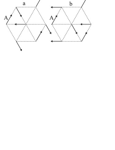
Figure 1: Two different magnetic structures on a hexagonal lattice possessing the same exchange energy. The direction of magnetic moment at point A is identical for both structures.

An especially interesting point to consider is a transition from a paramagnetic phase to a UUD structure occurring in a constant field on lowering the temperature. This is a transition into a collinear phase with an uncompensated magnetic moment. Such structures with uncompensated magnetic moment are characteristic of ferrimagnets, therefore for a description of this collinear phase on a triangular lattice a ferrimagnetic order parameter is used Miyashita . In ordinary ferrimagnets, however, the magnetic ions are located on non-equivalent crystallographic positions, which leads to the appearance of non-equivalent magnetic sublattices and an uncompensated moment. In these conventional ferrimagnets an ordering transition in an applied magnetic field is absent, as an induced moment exists at all temperatures. In the case of a 2D TLAM, however, all the magnetic ions are in equivalent positions, while the ordering into a UUD structure is accompanied by a tripling of the unit cell area, which causes a transition of a specific type Landau .

The majority of TLAMs have quasi one-dimensional character. These systems have been known and studied for some time nowCollins . 2D TLAMs demonstrating the properties described above are less common and have only recently become the subject of intense investigations. $\rm RbFe(MoO_{4})_{2}$ offers a rare opportunity to study a model system, which resembles closely an ideal 2D TLAM. The crystal structure of $\rm RbFe(MoO_{4})_{2}$ described by the space group $D_{3d}^{3}$ consists of layers of magnetic Fe³⁺ ions separated by (MoO₄)^2- groups and Rb⁺ ions. The $C^{3}$ axis is perpendicular to the layers. The magnetic Fe³⁺ ions form an equilateral triangular lattice within the layers, whereas along the $C^{3}$ axis they are interspaced by the Rb⁺ ions. Such a layered structure (depicted in References Klevtsov, and Klimin, ) ensures the magnetic two-dimensionality of $\rm RbFe(MoO_{4})_{2}$Klevtsov ; Svistov .

Relatively weak exchange interactions in $\rm RbFe(MoO_{4})_{2}$ allow one to reach the saturation field experimentally, while the large spin ($S=5/2$) of the magnetic Fe³⁺ ions justify a quasi classical description of the magnetic system. Previous experiments on powder and single crystal samples of $\rm RbFe(MoO_{4})_{2}$ established the presence of long range magnetic order below $T_{N}=3.8$ K and also demonstrated the stabilisation of the collinear structure around $M_{s}/3$ Inami ; Svistov . Specific heat measurements Jame gave estimates of the magnetic entropy change during the ordering process. The dynamics of low-frequency excitations probed by ESR measurements Svistov gave an estimate for the ratio of the intraplane to interplane exchange interactions as 25 and were also used to evaluate the magnetic anisotropy. By measuring the field and temperature dependence of the magnetisation Svistov and the specific heat Jame , the magnetic $H-T$ phase diagram was mapped out, the overall shape of which agreed well with the theoretical predictions for a 2D TLAM Korshunov ; Miyashita ; Kawamura ; Landau .

Neutron diffraction measurements performed in zero field Broholm2002 have found an ordered structure with a tripled in-plane period, which corresponds to a 120-degree configuration within the layers and an incommensurate ordering along the $C^{3}$ axis. NMR spectra of the ⁸⁷Rb ions located between the magnetic Fe³⁺ ions from neighbouring planes were reported in ref. NMR, . These spectra have allowed identification of various low-temperature phases: a structure with incommensurate modulation along the $C^{3}$ axis in low fields, a tilted commensurate structure and a UUD structure in higher fields.

This paper presents the results of a detailed investigation of the magnetic phase diagram and critical behaviour in the different phases of $\rm RbFe(MoO_{4})_{2}$ obtained by thermodynamic measurements. It also reports on the temperature dependence of the order parameter obtained by the ⁸⁷Rb NMR spectroscopy. The magnetic properties, phase diagram and critical indices demonstrate good quantitative agreement with the theoretical predictions for a classical 2D XY-model.

II Experimental details

Single-crystal samples of $\rm RbFe(MoO_{4})_{2}$ were synthesised by means of spontaneous crystallisation as described in Ref. Klevtsov, . The samples were thin (0.5 mm), nearly hexagonal plates with lengths along the edges up to 6 mm. The $C^{3}$-axis was found to be perpendicular to the surface of the plates for all samples. The results reported in this paper were obtained using samples produced by a significantly slower cooling of the melt compared to the samples used in Ref. Svistov, ; Jame, (1 K/hour vs 3 K/hour). This has resulted in samples with increased thickness and linear dimensions.

The magnetic moment was measured in a field of up to 12 T using an Oxford Instruments vibrating sample magnetometer. The heat-capacity measurements were performed by the standard heat-pulse method in the temperature range 0.4 to 40 K in a field of up to 9 T using a Quantum Design PPMS calorimeter equipped with a ³He option. NMR spectra of the ⁸⁷Rb ions ($I=3/2,\gamma=13.9312$ MHz/T) were recorded on the home-made spectrometer covering the range 35 to 114 MHz. The spin-echo signal was observed at constant frequency on sweeping the magnetic field in the range 2.5-9 T. Radio frequency pulses of 5 $\mu$s and 10 $\mu$s were separated by the time interval $\tau_{D}=50$ $\mu$s.

III Experimental results

III.1 Magnetisation and specific heat measurements

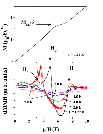
Figure 2: (Color online) Magnetisation curve versus field of a $\rm RbFe(MoO_{4})_{2}$ single crystal at $T=1.55$ K (top panel) and the derivative, $\frac{dM}{dH}$, taken at different temperatures (bottom panel). The field is applied perpendicular to the $C^{3}$-axis.

Field and temperature dependence of the magnetic moment of $\rm RbFe(MoO_{4})_{2}$ are shown in Figs. 2 and 3, respectively. The $M(H)$ and especially the $dM/dH$ curves show the $M_{s}/3$ plateau in the field range $(H_{c1},H_{c2})$ as well as an additional phase transition at $H_{c3}$ accompanied by a weak hysteresis. The obtained data are very similar to the $M(H)$ curves reported previously Svistov , apart from slightly reduced hysteresis effects around the $H_{c3}$ field and also a small (about 0.1 K) increase in the ordering temperature compared to the value of $T_{N}$ obtained on the batch of the samples studied beforehand.Svistov ; Jame ; Broholm2002 For this new sample batch, the relative amplitude of the susceptibility peak at $T_{N}$ has increased by a factor of two for small applied fields, which usually indicates an improved sample quality. The anomalies, singularities and other special points, which are seen in the curves in Figs. 2 and 3 and which correspond to various phase transitions are used to locate the positions of the phase boundaries, which are later summarised in the magnetic phase diagram (Fig. 11).

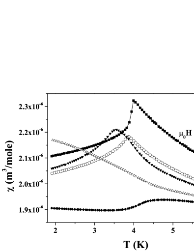
Figure 3: Temperature dependence of the magnetic susceptibility of a single crystal of $\rm RbFe(MoO_{4})_{2}$, ${\bf H}\perp C^{3}$ measured in different magnetic fields.

Fig. 4 shows the temperature dependence of the specific heat measured in $\rm RbFe(MoO_{4})_{2}$ for various values of a magnetic field applied in the basal plane of the crystal. The $C(T)$ curves demonstrate sharp anomalies corresponding to the phase transition from the high temperature paramagnetic phase to the low temperature magnetically ordered phase in every field from 0 to 9 T. For the $C(T)$ curves measured in the field interval 2.5 to 5.5 T, additional peaks are also observed when the external field coincides with the value of $H_{c1}$.

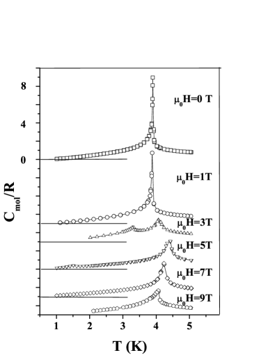
Figure 4: Temperature dependence of the specific heat measured in $\rm RbFe(MoO_{4})_{2}$, ${\bf H}\perp C^{3}$ measured in different magnetic fields. The curves are offset along the vertical axis.

Fig. 5 shows the field dependence of the specific heat measured at different temperatures (${\bf H}\perp C^{3}$). For temperatures below 4 K, sharp peaks associated with the start of the plateau at $H_{c1}$ are clearly seen on the $C(H)$ curves, while the phase transitions at $H_{c2}$ or $H_{c3}$ could not be detected here. For temperatures above 4.5 K, a wide and round maximum in $C(H)$ develops around a field of 5 T. On further heating, this maximum reduces in amplitude and becomes undetectable above 8 K. The observed peak positions were plotted on the phase diagram (Fig. 11) together with the data obtained from the magnetisation measurements.

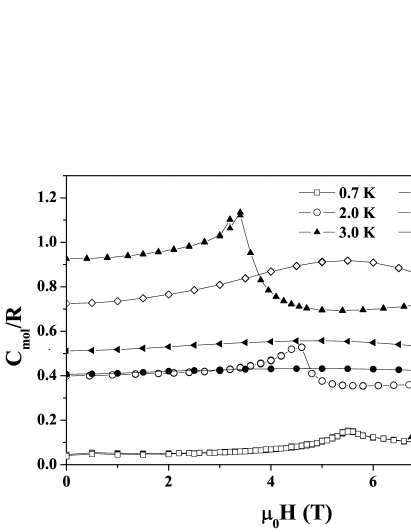
Figure 5: Field dependence of the specific heat of $\rm RbFe(MoO_{4})_{2}$ measured for ${\bf H}\perp C^{3}$ for various temperatures.

As can be seen from Fig. 4, the application of a weak magnetic field reduces marginally the ordering temperature. However, when the field is strong enough to stabilise a collinear phase, the ordering temperature develops a non-monotonic dependence with applied field. It rises with field for $H>H_{c1}$ reaching a maximum of 4.5 K at $H=5$ T. This maximum value exceeds significantly the zero-field ordering temperature of 3.9 K.

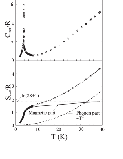
Figure 6: Temperature dependence of the specific heat (top panel) and the entropy (bottom panel) measured in $\rm RbFe(MoO_{4})_{2}$ in zero field. The dashed and solid lines correspond to the lattice and the magnetic contributions to the entropy.

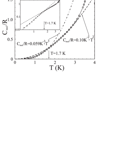
Figure 7: Temperature dependence of the specific heat of $\rm RbFe(MoO_{4})_{2}$ in the low-temperature region. A crossover from a square to a cubic temperature dependence is clearly visible on the log-log plot (the inset).

The top panel of Fig. 6 shows the temperature dependence of the specific heat measured in $\rm RbFe(MoO_{4})_{2}$ for a wide temperature interval in zero magnetic field. For temperatures in the region $10-40$ K, the specific heat follows a $T^{2}$-type of the temperature dependence. As this dependence is observed both below and above the Weiss temperature, $\theta_{CW}=25$ K, it is reasonable to suggest that it corresponds mostly to lattice vibrations. Extrapolation of the lattice contribution down to zero temperature shows that for $T<5$ K, the magnetic contribution to the specific heat is dominant and that the lattice contribution can be neglected. The temperature dependence of the entropy obtained by integrating the $C(T)/Tvs\;T$ curves is shown in the bottom panel of Fig. 6. By subtracting the lattice contribution (the dashed line) one can obtain the temperature dependence of the magnetic entropy, shown in Fig. 6 as a solid line. At temperatures exceeding several times the ordering temperature $T_{N}$ the magnetic entropy tends to a value agreeing well with ${\rm R}ln(2S+1)={\rm R}ln6$.

Fig. 7 shows temperature dependence of the zero-field specific heat of $\rm RbFe(MoO_{4})_{2}$ in the low-temperature region. For $T<1.7$ K the temperature dependence of the specific heat is described well by the regular cubic law (shown by the dash-dotted line in Fig. 7), while in the temperature interval 1.7 to 3.4 K it follows a quadratic dependence (shown by the dashed line). The inset in Fig. 7 reproduces the same data on a double logarithmic scale.

III.2 NMR ⁸⁷Rb spectra

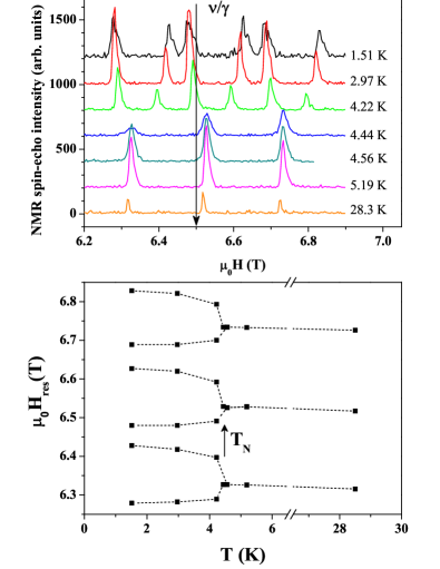
Figure 8: (Color online)NMR spectra of $\rm RbFe(MoO_{4})_{2}$ recorded for a frequency of 90.6 MHz at various temperatures, $\mathbf{H}\perp C_{3}$ (top panel). Bottom panel shows the temperature dependence of the resonance fields.

The NMR ⁸⁷Rb spectra were recorded in the frequency range 35-115 MHz for various temperatures. Typical temperature evolution of the spectra is illustrated in Fig. 8, where the top panel shows the field dependence of the spin-echo signal at different temperatures and the bottom panel shows the temperature dependence of the resonance fields. In the paramagnetic phase, the NMR spectrum consists of three lines, with the central line corresponding to the ($-1/2\leftrightarrow 1/2$) transition and the two satelites to the ($-3/2\leftrightarrow-1/2$) and ($1/2\leftrightarrow 3/2$) transitions. The frequency difference for these transitions is caused by the quadrupole splitting, which is found to be temperature independent over the entire temperature range under investigation. The description and interpretation of the NMR spectra in $\rm RbFe(MoO_{4})_{2}$ and also their relation with the magnetic structure are given in our earlier paper NMR . As was shown in that paper, the value of the NMR frequency in $\rm RbFe(MoO_{4})_{2}$ is determined mostly by the external magnetic field, by the quadrupole splitting and also by the dipolar field created by the magnetic ${\rm Fe^{3+}}$ ions on ⁸⁷Rb nuclei, while the contribution from the hyperfine field is negligibly small.

In the paramagnetic phase, on lowering the temperature, all three NMR lines shift slightly towards higher fields and also broaden while approaching the ordering temperature $T_{N}$. The shift is caused by the dipolar field created on Rb sites by the field-induced magnetic moments of the ${\rm Fe^{3+}}$ ions.

In the magnetically ordered phases, the dipolar fields of the Fe ions make the Rb ion positions non-equivalent, which results in splitting of all the spectral components into pairs of lines with distinct intensity. The more intense line shifts towards lower field, while the less intense line shifts towards higher field. The ratio of the intensities for these lines is approximately 2 to 1. The observed splitting can be used for a precise determination of the Neel temperature; it is also useful in choosing an appropriate model for the magnetic structure of $\rm RbFe(MoO_{4})_{2}$NMR . The values of the ordering temperatures, as inferred from the NMR results, are also collected in Fig. 11 together with the magnetisation and specific heat points.

In order to determine the temperature dependence of the order parameter, detailed NMR measurements were performed near the critical temperature for one of the spectral components. This component is seen at a frequency of 81 MHz in a field of 5.82 T, which is nearly in the centre of the collinear phase. The values of the resonance fields for a central line above and below its splitting point are plotted in Fig. 9.

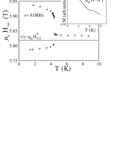
Figure 9: Temperature dependence of the NMR resonance field $B_{res}(T)$ and the magnetic moment $M(T)$. $\mu_{0}H\simeq 6$ T, ${\bf H}\perp C_{3}$.

Let us define here the order parameter in the collinear phase following Ref. Miyashita2, :

${\bf\eta}=(({\bf M}_{1}+{\bf M}_{2})/2)-{\bf M}_{3})/2$,
where ${\bf M}_{1}$, ${\bf M}_{2}$ and ${\bf M}_{3}$ are the magnetic moments of the three sublattices normalised per magnetic ion. The parameter $\eta$ is zero in the paramagnetic phase and nonzero in the ordered collinear phase. Let us also introduce a normalised full magnetic moment:

${\bf\mu}=({\bf M}_{1}+{\bf M}_{2}+{\bf M}_{3})/3$.

The temperature dependence of the order parameter $\eta$ can be established by measuring the local field $B_{eff}$, which is created by the Fe³⁺ ions on the Rb nuclei. Experimentally, this field is defined as

$B_{eff}=B_{res}-\nu/\gamma-\Delta\nu^{q}/\gamma$,
where $\Delta\nu^{q}$ is the quadrupole shift of the resonance field.

At any finite temperature the magnetic structure can be represented as a superposition of the ferromagnetic and collinear (UUD) states with the corresponding weights $\mu-\eta/3$ and $\eta$, respectively. Therefore, the effective field $B_{eff}$ consists of two components, one of them being proportional to $\mu$, and the other being proportional to $\eta(T)$. The order parameter is hence given by the expression

$\eta(T)\sim B_{eff}(T)-B_{eff}(T_{0})\cdot M(T)/M(T_{0})$,
where $T_{0}$ is a fixed temperature above the ordering temperature $T_{N}$. From this expression, by using the independently measured temperature dependence of the magnetic moment, one can determine the order parameter. Fig. 9 gives the temperature dependence of the NMR resonance field as well as of the magnetic moment $M(T)$ measured in a field of $\simeq 6$ T. Fig. 10 shows the temperature dependence of the order parameter obtained using the data of Fig. 9 as described above. An absolute value of the order parameter is obtained by using the results of Ref. NMR, , where the value of $\eta$ was determined for $T=1.6$ K and a magnetic field of 6 T. An abrupt change in the order parameter is clearly seen near the ordering temperature.

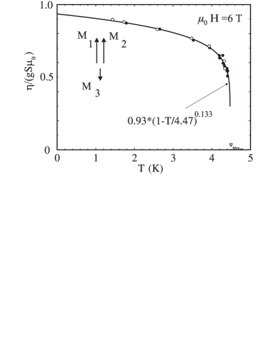
Figure 10: Temperature dependence of the order parameter $\eta$. The solid and open circles correspond to the values of $\eta$ obtained from the resonance fields of ⁸⁷Rb residing in different positions with respect to the magnetic structure. The triangles correspond to the values of $\eta$ in the paramagnetic phase. $\mu_{0}H\simeq 6$ T, ${\bf H}\perp C_{3}$.

III.3 Magnetic phase diagram

Fig. 11 summarises the positions of the phase boundaries in $\rm RbFe(MoO_{4})_{2}$ for a field applied in the basal plane of the crystal, determined by using different methods. In weak fields, the transition temperature is well defined (with the accuracy better than 0.1 K) from the magnetisation and specific heat measurements. The phase boundary between the paramagnetic and the collinear phase (P3 in Fig. 11) is also well defined by the peak in the specific heat and by the splitting in the NMR spectrum, while the magnetisation curve shows a smooth behaviour. The phase boundaries corresponding to the transition fields $H_{c2}$ and $H_{c3}$ are only visible in the magnetisation curves, whereas the anomaly at $H_{c1}$ is clearly seen in both the specific heat and the magnetisation curves.

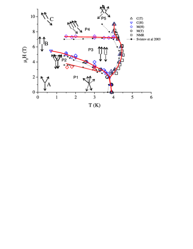
Figure 11: (Color online)Magnetic phase diagram of $\rm RbFe(MoO_{4})_{2}$ for $\mathbf{H}\perp C_{3}$ determined by using different experimental methods. Spin structures of magnetic layers are schematically presented by solid arrows and marked as A, B, C. Two-layer fragments of supposed 3D spin structures are shown by solid and dashed arrows for different magnetic phases marked as P1-P5, see text.

The dashed lines in Fig. 11 represent the phase boundaries obtained in our earlier paper Svistov . Although the overall agreement between the two sets of the results is good, a noticeable difference between the transition temperatures is most likely to be caused by the variations in sample quality, originating from difference in the sample preparation procedures. The specific heat peaks associated with the phase transition from the paramagnetic to the collinear phase were much sharper for the new batch of samples, for which the NMR signal splitting also occurs over a narrower temperature interval. During the measurements with different samples from the same growth batch it has been noticed that by rigidly gluing the NMR sample to a sample holder it was possible to broaden significantly the phase transition region. In addition, the specific heat measurements (performed as usual for the heat-pulse method with the crystals attached rigidly to a platform using a low-temperature grease) show that the peaks in $C(T)$ measured for the PM to P3 transition in the thinner and therefore more stressed samples were about 0.2 K broader compared to the thicker and less stressed samples. It should be added, however, that the shape and the width of the peaks in $C(T)$ curves were not sensitive to the stress for the other magnetic phases (above and below the phase with a collinear structure).

IV Magnetic phase diagram for $H\parallel C^{3}$

Fig. 12 (upper panel) shows the temperature dependence of the specific heat measured in $\rm RbFe(MoO_{4})_{2}$ for ${\bf H}\parallel C^{3}$. The lower panel also shows the records of the central quadrupolar-split NMR line measured at 35 MHz for the same direction of the field. When the field is applied along the $C^{3}$-axis (“hard” axis in terms of the magnetic anisotropy), a single phase transition into a magnetically ordered phase is observed via a $\lambda$-like anomaly in $C(T)$. This transition is seen as a sharp maximum in the $C(H)$ curves (not shown) and also as a splitting of the NMR line. For ${\bf H}\parallel C^{3}$, this splitting is nearly an order of magnitude smaller compared to the ${\bf H}\perp C^{3}$ geometry.

The $H-T$ phase diagram for a field applied along the $C^{3}$-axis is shown in Fig. 13. The circles correspond to the phase boundary positions obtained from the specific heat measurements, while the square marks the phase transition observed by the NMR splitting.

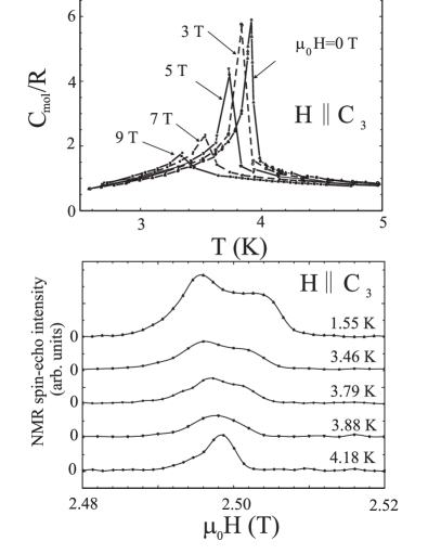
Figure 12: Temperature dependence of the specific heat in different fields (top panel) and spectra of the central quadrupole-split NMR line measured at 35 MHz for different temperatures (bottom panel). The field is applied along the $C^{3}$ axis of the $\rm RbFe(MoO_{4})_{2}$ single crystal.

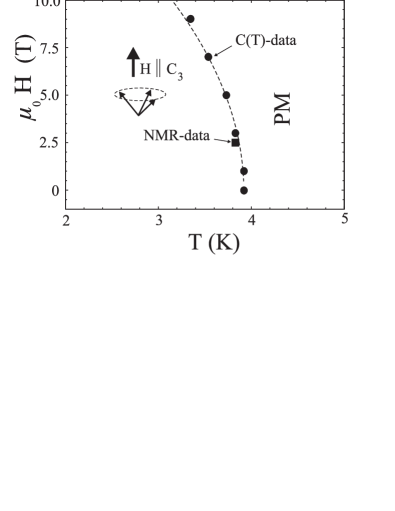
Figure 13: The magnetic phase diagram of the $\rm RbFe(MoO_{4})_{2}$ single crystal for $\mathbf{H}\parallel C^{3}$. The dashed line corresponds to the relation $\mu_{0}$H $=20.2$ T $\times(1-T/3.9$ K$)^{0.5}$. The value of the experimental uncertainty in the position of the phase boundary is represented by the markers size.

V Discussion

V.1 Initial aspects

Here we discuss the observed phase transitions in $\rm RbFe(MoO_{4})_{2}$ and its critical properties. Apart from the data presented in this paper, the discussion will be based on the available data on the microscopic structure of $\rm RbFe(MoO_{4})_{2}$ obtained from neutron diffraction Broholm2002 and NMR NMR experiments, as well as on the established hierarchy of the magnetic interactions Svistov : the intralayer exchange, the easy-plane anisotropy and the interlayer exchange. Besides these experimental facts we shall use the results of the calculation of the dipole energy, which can help to select between the proposed states with equal nearest neighbors exchange energy.

It has to be noted that in zero field and at finite temperature for the case of an ideal two-dimensional system, long range order of the magnetic components is prohibited by the Mermin-Wagner theorem. For a triangular lattice with antiferromagnetic exchange interactions, however, apart from the Berezinskii-Kosterlitz-Thouless transition there should be an additional transition to a state with long-range order with the chirality parameter for the neighbouring triangles, the so-called “staggered helicity (vorticity)” state Miyashita ; Korshunov . Monte Carlo simulations for this state Miyashita show that this phase is close to the state with long-range order of the nonzero average magnetic moments, as the spin-spin correlations decay in a power-law manner. Moreover, the characteristic relaxation time for the 120-degree three-sublattice structure could be relatively long and may exceed the dynamical range for various experimental techniques.

Computer simulations show the presence of chiral ordering both for the 2D XY-model Landau and 2D Heisenberg system.Miyashita ; Miyashita2 For the 2D XY-model, in addition to the paramagnetic phase, the $H-T$ phase diagram contains the three ordered phases,Landau which have previously been identified in, for example, Ref. Korshunov, . These structures are depicted and labelled as A, B and C in Fig. 11.

In the presence of an external magnetic field, the stabilisation of long range order becomes inevitable Korshunov . Computer simulations for the Heisenberg spins Miyashita ; Miyashita2 reveal qualitatively similar results to the XY-model phase diagram, however, the exact positions of the phase boundaries are determined there far less accurately. Both models predict a characteristic non-monotonic variation of the ordering temperature with the magnetic field. The simulation results for the XY-model are shown in Fig. 14.

Weak interlayer exchange coupling should, in the general case, facilitate the appearance of 3D long range order. Given the results for the 2D models discussed above and the proximity of the ground states for these systems, one can speculate that the temperature of the 3D ordering should be close to the critical temperature of the 2D transition. In order to corroborate this conjecture, additional Monte Carlo simulations for the system with a finite interlayer exchange and magnetic anisotropy would be required.

In order to analyse the real structures in 3D crystals one has to take into account the interlayer exchange coupling and to consider various possibilities for the alignment of the spins in the neighbouring planes. Theoretical analysis of the different allowed structures for an antiferromagnetic interlayer exchange has been performed in Ref. Gekht, . The proposed magnetic phases have then been used as the models for $\rm RbFe(MoO_{4})_{2}$ in Ref. Svistov, . Fig. 11 shows the spin configurations of the ordered phases, which have been selected from the proposed list Gekht on the basis of matching the NMR-detected commensurate-incommensurate transition NMR , magnetisation plateau, and possible periodicity along $C^{3}$ direction, which is discussed below. Solid and dashed arrows in Fig. 11 represent the orientations of the magnetic moments of the Fe³⁺ ions from neighboring planes for these selected configurations.

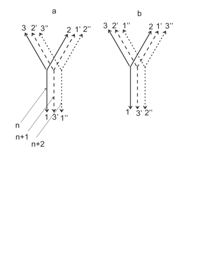
Figure 15: Schematic representation of the magnetic structures with different periodicity along the $C^{3}$-axis: $2c$ on the left (a) and $3c$ on the right (b). Solid and dashed arrows correspond to the direction of the magnetic moments in the neighbouring planes. Numbers 1, 1’ and 1” mark the magnetic moments of the Fe³⁺ ions located above one another in the neighbouring $n^{th}$, $n+1^{st}$ and $n+2^{nd}$ magnetic layers.

Let us consider the procedure of the selection of the proposed structures. One should note that for the spin structures with two parallel sublattice magnetisations within a layer (e.g. structures suggested for phases P2,P3,P4), an interlayer exchange does not define the magnetic periodicity along the $C^{3}$-axis, which could therefore be any integer multiple of the lattice periods. This point is illustrated in Fig. 15, where the two structures with the periodicity along the $C^{3}$-axis equal $2c$ and $3c$, contain the same number of various angle combinations for the neighbouring spins. These two structures thus possess the same exchange energy. This periodicity must be due to some other interactions, that are weaker when compared to the exchange coupling. Among the possible candidates for the interactions which select a period along $C^{3}$ axis are the dipole-dipole interactions and further neighbour exchange interactions along the $C^{3}$-axis. The direct calculation of the dipole energy shows that it is lower for the period of $3c$. This gain in the dipole energy equals approximately 0.4 mK per Fe-ion for UUD structure. Therefore we suppose that the structures suggested for phases P2, P3, P4 have the period $3c$. The next-nearest antiferromagnetic exchange interaction in the $C^{3}$ direction would also result in the preference of period $3c$.

Fig. 11 shows results of the various experimental techniques that reveal the presence of five ordered phases. The phase transition, corresponding to the field $H_{c3}$, which is marked in the $\frac{dM}{dH}$ curves in Fig. 2 is an incommensurate-commensurate transition indicated by the characteristic change of the NMR spectrum NMR . We suppose that the incommensurate structure below $H_{c3}$ corresponds, as usual, to a nearly antiparallel orientation of spins from neighboring layers (structure $P1$), this structure being rotated around the $C^{3}$ axis by a small angle from layer to layer. In the range above $H_{c3}$ the commensurate structure takes place for the phase P2. In Ref. Svistov, , two possible variants were proposed for the spin structures in phases $P1$ and $P2$ based on the results of theoretical considerations Gekht ; Korshunov2002 . We selected for the phase $P2$, the structure which allows the period of $3c$, favorable for dipole-dipole energy. For the phase $P1$ the structure, compatible with period $2c$ is suggested, since for the typical incommensurate structures in antiferromagnets the orientation of spins in neighboring layers should be close to antiparallel one, like at the period value $2c$.

In the phase $P3$, i.e. in the plateau range, the collinear structure within a layer and the periodic structure along $C^{3}$-axis, probably with the period $3c$, is realised. The structures of P4 or P5 type may be proposed for the high-field range between $H_{c2}$ and saturation. We have here no NMR data which could distinguish between commensurate and incommensurate states, thus we can not determine the nature of the P4-P5 boundary, detected by small $dM/dH$ singularity in RefSvistov . Nevertheless, if we extrapolate the period value of $3c$ from $P3$ to $P4$ , the structure which is compatible with period $3c$ should be selected, as shown in Fig. 11. In this case the transition to the second high-field spin structure of the phase $P5$ should change the period to $2c$ or again result in the incommensurate modulation.

The collinear structure of the $P3$ phase may be taken as determined most precisely, as it corresponds to the maximum value of the NMR shift NMR , which is maintained in the entire field range $H_{c1}<H<H_{c2}$. The spin structures of other phases are suggested as probable configurations.

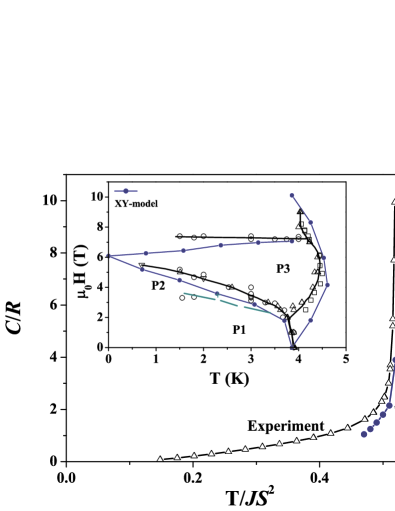
Figure 14: (Color online) Experimental (open symbols) and theoretical Landau (solid symbols) temperature dependence of the specific heat in $\rm RbFe(MoO_{4})_{2}$ plotted against the normalised temperature in zero field. The inset shows the $H-T$ phase diagram for $\bf{H}\perp C_{3}$, where the open symbols represent the experimental results as in Fig. 11, solid symbols are the results of computer simulations Landau with $J=1.23$ K. The solid lines in the inset are drawn as a guide to the eye.

V.2 2D-3D crossover of the specific heat temperature dependence

The overall shape of the phase diagram, as well as the characteristic widening of the collinear phase range with increasing temperature predicted in Ref. Korshunov, points to the two-dimensional nature of magnetism in $\rm RbFe(MoO_{4})_{2}$. Here, we show that the observed change-over in the temperature dependence of the specific heat from the low-temperature $T^{3}$ law to the intermediate temperature $T^{2}$ law (as described in section III.1) is also indicative of the two-dimensional disposition of this magnetic system.

The temperature dependence of an antiferromagnet for $T<0.6\;T_{N}$ is usually determined by thermally activated magnons. The spectrum of acoustic magnons in antiferromagnetic $\rm RbFe(MoO_{4})_{2}$ consists of one gapless mode and two modes with a gap of 90 GHz (4.5 K).Svistov At such low temperatures, the variation of the gap’s magnitude should be small, as the order parameter for $T<0.6\;T_{N}$ is reduced by not more than 30%. The main contribution to the specific heat in this temperature region comes from the magnons of the gapless branch. At the lowest temperature the wave-numbers of the thermal magnons are small and lie far away from the Brillouin zone boundary. Therefore one can expect for $C(T)$ a typical three-dimensional behaviour, that is $C(T)\sim T^{3}$.

Due to a large difference between the inter- and the intra-layer exchange interactions, the magnon dispersion relation is highly anisotropic – the magnons propagating along the $C^{3}$-axis are less dispersive than those with a wave-vector confined to the triangular plane. Consequently, at a certain temperature, the energy of the thermal magnons travelling along the $C^{3}$-axis reaches its maximum value, while the size of the $k$-space region corresponding to magnons with $k\perp C^{3}$ will continue to expand. For these temperatures one can expect a typical two-dimensional behaviour, that is $C(T)\sim T^{2}$. Inevitably, the change-over from a cubic to a quadratic law should occur at the temperature dependent on interlayer exchange energy, or, more precisely, on the maximum energy of the $k||C^{3}$ magnons of the lowest gapless branch. This is the energy of the lowest “exchange”-mode of the antiferromagnetic resonance spectrum. According to Ref. Svistov, , the gap of the lowest exchange mode is about 30 GHz (1.5 K), which agrees well with the observed crossover temperature. Thus the 2D-3D crossover in the temperature dependence of specific heat confirms the domination of two-dimensional features in the thermodynamic behaviour of $\rm RbFe(MoO_{4})_{2}$.

V.3 Critical properties of the magnetic ordering transition for ${\bf H}\perp C^{3}$

Given the two-dimensional nature of the magnetic properties of $\rm RbFe(MoO_{4})_{2}$, let us compare the observed critical behaviour with the results of the classical Monte Carlo simulations Landau performed for the 2D XY-model. The Neel temperature in this simulation is defined as $0.5JS^{2}$. Using the value of $J=1.2\pm 0.1$ K determined from the susceptibility and saturation magnetisation measurements Svistov ; Inami , the predicted ordering temperature is $3.75\pm 0.3$ K, which is in a good agreement with the value of $T_{N}=3.85\pm 0.05$ K determined experimentally. The ordering temperature for the 2D Heisenberg antiferromagnet on a triangular lattice, on the other hand, is defined as $0.35JS^{2}$, Miyashita2 which unexpectedly gives less satisfactory agreement with the experimental $T_{N}$.

Fig. 14 shows the comparison between the temperature dependence of the specific heat measured experimentally and obtained from the Monte Carlo simulations Landau . It also shows a comparison of the phase boundary positions from the experimental $H-T$ diagram (see Fig. 11) and the simulations Landau for $\bf{H}\perp C^{3}$. For the theoretical curve, the value of the exchange parameter quoted above has been used. The overall agreement is satisfactory, as the two phase diagrams have very similar shapes, apart from the low-field region. For low fields, however, the distinction is fundamental: the theoretical model predicts a phase transition from paramagnetic to chiral structures only through a collinear phase, while experimentally a single phase transition is observed for all fields below 2 T.

The measured $C(T)$ and $\eta(T)$ curves allow one to determine the specific heat and the order parameter critical indices for the phase transition into the collinear phase. Corresponding experimental data are presented in Figs. 10 and 16. The experimentally determined indices are $\alpha=0.40\pm 0.03$ for the specific heat and $\beta=0.13\pm 0.02$ for the order parameter. They agree well with $\alpha=1/3$ and $\beta=1/9$ obtained from the simulations Landau .

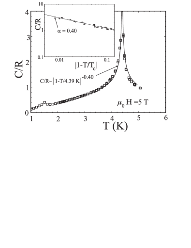
Figure 16: Temperature dependence of the specific heat for a field of $\mu_{0}H=5$ T applied in the easy-plane of $\rm RbFe(MoO_{4})_{2}$. The inset shows $C\;vs\;|1-T/T_{c}|$ curve in the vicinity of the phase transition on a log-log scale.

It can be concluded then that the ordering temperature, the magnetic phase diagram and the critical indices of the specific heat and the order parameter demonstrate a satisfactory quantitative agreement with the 2D XY-model predictions for zero field and also for regions of the field ($H\perp C^{3}$) where the collinear phase is stable. Most likely this agreement can be explained by the large value of the energy gap for the magnon branch, which corresponds to a deviation of the spins out of the basal plane.

This gap has been estimated as 90 GHz (or 4.5 K) Svistov . Therefore, for all the magnetically ordered phases, the thermodynamic properties are defined by gapless and low-energy magnons, corresponding to spin fluctuations within the easy plane. This, in turn, justifies the applicability of the XY model.

V.4 Phase diagram for $\bf H\parallel C^{3}$

The easy-plane type of magnetic anisotropy in $\rm RbFe(MoO_{4})_{2}$ is confirmed by the observation of the magnetisation plateau around $M_{s}/3$ for the magnetic field applied in the $ab$ plane and by the linear rise of the $M(H)$ curves for the field parallel to the $C^{3}$-axis. For an easy-plane anisotropy, the magnetic moment of the system is generated for $H\parallel C^{3}$ by the even tilts of all the subblattices in an umbrella-like structure towards the field (see Fig. 13). For such a system, the application of an external magnetic field should result in a decrease of the ordering temperature. Moreover, in the vicinity of $T_{N}(H=0)$, the reduction should be proportional to the square of the field, similarly to an ordinary two-sublattice antiferromagnet LandauLifshitz . The dashed line in Fig. 13 shows such a dependence, $H_{c}=a(1-T/T_{c})^{0.5}$, with $a=20.2$ T and $T_{c}=3.9$ K. For the case of the uniformly tilted spins described here, splitting in the NMR spectra should be absent, but it is observed. The origin of this small but clearly visible splitting remains unknown at the present time.

VI Conclusions

To summarise, we have performed a systematic and comprehensive study of the thermodynamic and magnetic properties of the quasi two-dimensional TLAM $\rm RbFe(MoO_{4})_{2}$, as well as measurements of the magnetic order parameter for this compound. A crossover from a $T^{2}$ law to a $T^{3}$ law is observed for the temperature dependence of the specific heat at low temperatures. The phase diagram and critical properties demonstrate a surprisingly good quantitative agreement with the predictions for the XY-model despite the fact that the easy-plane anisotropy in $\rm RbFe(MoO_{4})_{2}$ does not dominate the main exchange interaction.

The authors are grateful to S.E. Korshunov, V.I. Marchenko, M.E. Zhitomirsky, A. Loidl, H.-A. Krug von Nidda for discussions and to M.R. Lees for a critical reading of the manuscript. This work is supported by the Grant 04-02-17294 Russian Foundation for Basic Research, RF President Science Schools Program, contract BMBF №VDI/EKM 13N6917-A, program of the German research society Sonderforschungsbereich 484 (Augsburg), and the EPSRC grant (University of Warwick). The work of L.E. Svistov is supported by the Alexander von Humboldt fellowship.

References

- (1) M.F. Collins and O.A. Petrenko, Can. J. Phys. 75, 605 (1997).
- (2) S. Nakatsuji, Y. Nambu, H. Tonomura, O. Sakai, S. Jonas, C. Broholm, H. Tsunetsugu, Y. Qiu and Y. Maeno, Science 309, 1697 (2005).
- (3) H. Kawamura, J. Phys. Soc. Jpn. 54, 3220 (1985).
- (4) D.H. Lee, J.D. Joannopoulos, J.W. Negele and D.P. Landau, Phys. Rev. B 33, 450 (1985).
- (5) A.V. Chubukov and D.I. Golosov, J. Phys. Condens. Matter 3, 69 (1991).
- (6) R.S. Gekht and I.N. Bondarenko, Zh. Eksp. Teor. Fiz. 111, 627 (1997) [JETP 84, 345 (1997)].
- (7) E. Rastelli and Tassi, J. Phys. Condens. Matter 8, 1811 (1996).
- (8) S.E. Korshunov, J.Phys.: Solid State Phys. 19, 5927 (1986).
- (9) H. Kawamura and S. Miyashita, J. Phys. Soc. Jpn. 53, 4138 (1984).
- (10) R.F. Klevtsova and P.V. Klevtsov, Kristallografiya 15, 953 (1970) [Russian Crystallography].
- (11) S.A. Klimin, M.N. Popova, B.N. Mavrin, P.H.M. van Loosdrecht, L.E. Svistov, A.I. Smirnov, L.A. Prozorova, H.-A. Krug von Nidda, Z. Seidov, A. Loidl, A.Ya. Shapiro and L.N. Demianets, Phys. Rev. B 68, 174408 (2003).
- (12) L.E. Svistov, A.I. Smirnov, L.A. Prozorova, O.A. Petrenko, L.N. Demianets and A.Ya. Shapiro, Phys. Rev. B 67, 094434 (2003).
- (13) T. Inami, Y. Ajiro and T.Goto, J. Phys. Soc. Jpn. 65, 2374 (1996).
- (14) G.A. Jorge, C. Capan, F. Ronning, M. Jame, M. Kenzelmann, G. Gasparovich, C. Broholm, A.Ya. Shapiro and L. N. Demianets, Physica B 354, 297 (2004).
- (15) G. Gasparovich, M. Kenzelmann, C. Broholm, L. N. Demianets, A. Ya. Shapiro, private communication 2002, unpublished
- (16) L.E. Svistov, L.A. Prozorova, N. Buttgen, A.Ya. Shapiro and L.N. Dem’yanets, JETP Letters 81, 102 (2005).
- (17) H. Kawamura and S. Miyashita, J. Phys. Soc. Jpn. 54, 4530 (1985).
- (18) S.E. Korshunov, private communication (2002).
- (19) Electrodynamics of Continuous Media by E.M. Lifshitz, L.D. Landau and L.P. Pitaevskii, (Landau and Lifshitz Course of Theoretical Physics, Volume 8, Oxford, Butterworth-Heinemann, 1995).