Intense terahertz laser fields on a quantum dot with Rashba spin-orbit coupling

Abstract

We investigate the effects of the intense terahertz laser field and the spin-orbit coupling on single electron spin in a quantum dot. The laser field and the spin-orbit coupling can strongly affect the electron density of states and can excite a magnetic moment. The direction of the magnetic moment depends on the symmetries of the system, and its amplitude can be tuned by the strength and frequency of the laser field as well as the spin-orbit coupling.

The study of semiconductor based opto-electronics, which combines the ultrafast electronics with the low-power optics, has been fruitfully carried out for years. Schemes based on semiconductor quantum dots (QD’s) have been proposed and actively studied in order to realize the more ambitious goal of quantum opto-electronic devices, which provide interface between quantum bits (qubits) and single-photon quantum optics and can perform quantum information processing and communication on one chip. Single spins in QD’s are natural candidatesLoss1 ; Loss2 ; Loss3 for qubits as they have long coherence times and can be manipulated both electronically and optically. There are many theoretical works on spin relaxation/decoherence and manipulation in QD’s.LossDot ; spintronics ; das ; wang Experimental realization of the electrical/optical generation and read-out of single spin in QD have also been carried out.readout1 ; readout2

The spin-orbit coupling (SOC) plays an essential role in the dynamics of electron spins in QD’s. It enables the electrical manipulation by tuning the gate voltage but also leads to the spin relaxation/decoherence together with the different scattering mechanism such as the electron-phonon scattering.LossDot In addition to the above effects, the SOC in QD’s causes a spin splitting of a few meV, the order of terahertz (THz), and therefore is expected to affect the response of electrons in QD’s to the THz laser. The effect of the SOC on far-infrared optical absorption spectrum has been discussed in detail by Rodriguez et al.Rodriguez Until recently, the study on the response to the THz radiation has been focused on the spin-unrelated problems such as the dynamic Franz-Keldysh effect (DFKE),Yacoby ; Jauho ; Jauho2 ; Nordstrom the AC Stark effectNordstrom ; AH and the photo-induced side-band effect.Cerne ; Kono ; Phillips ; PR1 ; PR2 ; Arrachea Very recently Cheng and Wu discussed the effects of intense THz laser field on a two dimensional electron gas (2DEG) with the Rashba SOC.cheng_2005_APL It is demonstrated that the laser field can significantly modify the density of states (DOS) of the 2DEG and induce a finite off-diagonal density of spin polarization which indicates the strong correlation of different spin branches. Later Wang et al. discussed the time-dependent spin-Hall current in the 2DEG driven by an intense THz field.Wang_Lei How the intense THz laser affects the QD’s in the presence of the SOC needs to be further revealed. In this paper, we study the effect of intense THz laser on semiconductor QD’s with the Rashba SOC.Rashba

We consider a quantum dot grown in an InAs quantum well with growth direction along the $z$-axis. A uniform radiation field (RF) ${\mathbf{E}}(t)={\mathbf{E}}\cos(\Omega t)$ is applied along the $x$-axis with the period $T_{0}=\frac{2\pi}{\Omega}$. By using the Coulomb gauge, the Hamiltonian is written asWinkler

$$H(t)=\frac{{\mathbf{P}}^{2}}{2m^{\ast}}+V_{c}({\mathbf{r}})+H_{so}(\mathbf{P}).$$ (1)

Here the momentum ${\mathbf{P}}=-i\mbox{\boldmath$\nabla$\unboldmath}+e{\mathbf{A}}(t)$ with $\mathbf{A}(t)=-\mathbf{E}\sin(\Omega t)/\Omega$ being the vector potential; $m^{\ast}$ is the electron effective mass. The confining potential of the quantum dot is taken to be $V_{c}({\mathbf{r}})=\frac{1}{2}m^{\ast}\omega_{0}^{2}r^{2}$ in the $x$-$y$ plane. An infinite-well-depth assumption is made along the $z$-axis and the well width is assumed to be small enough so that only the lowest subband is relevant. $H_{so}$ is the SOC which is composed of the Rashba termRashba and the Dresselhaus term.Dresselhaus For InAs quantum well, the Rashba term is the dominant one. $H_{so}({\mathbf{P},t})=\alpha_{R}[\hat{\sigma}_{x}{P}_{y}-\hat{\sigma}_{y}{P}_{x}]$ with $\hat{\sigma}$ denoting the Pauli matrix and $\alpha_{R}$ representing the Rashba SOC parameter which can be tuned by gate voltage up to the order of 4$\times 10^{-9}$ eV$\cdot$cm.Grundler ; Sato

By employing the Floquet theorem, the solution to the Schrödinger equation with time-dependent Hamiltonian (1) can be written as,shirley

$$\Psi_{\lambda}({\bf r},t) = e^{-i[E_{em}t-\gamma\sin(2\Omega t)]}$$ (2)

$$\times e^{-i\varepsilon_{\lambda}t}\sum_{n=-\infty}^{\infty}\sum_{\alpha}F_{n\alpha}^{\lambda}\phi_{\alpha}({\bf r})e^{in\Omega t}\ .$$

Here $E_{em}=\frac{e^{2}E^{2}}{4m^{\ast}\Omega^{2}}$ is the energy induced by the RF due to the DFKE;Jauho ; Jauho2 $\gamma=E_{em}/2\Omega$; $\{\phi_{\alpha}({\mathbf{r}})\}$ can be any set of complete basis. $\{F_{n\alpha}^{\lambda}\}$ are the eigenvectors of the equations: shirley

$$\sum_{m=-\infty}^{\infty}\sum_{\beta}\langle\alpha n|{\cal H_{F}}|\beta m\rangle F_{m\beta}^{\lambda}=\varepsilon_{\lambda}F_{n\alpha}^{\lambda}\ ,$$ (3)

in which $\langle{\bf r},t|\alpha n\rangle\equiv\phi_{\alpha}({\bf r})e^{in\Omega t}$, ${\cal H_{F}}=H(t)-i\partial_{t}$ and $\langle\alpha n|{\cal H_{F}}|\beta m\rangle=H_{\alpha\beta}^{n-m}+m\Omega\delta_{\alpha\beta}\delta_{nm}$ with $H^{n}=\frac{1}{T_{0}}\int_{0}^{T_{0}}\!\!d{t}e^{-in\Omega t}H(t)$ representing the $n$-th Fourier component of the Hamiltonian. The eigen-values $\varepsilon_{\lambda}$ of the equations are solved in the region $(-\Omega/2,\Omega/2]$.shirley In the case of the Rashba SOC, the non-zero terms are

$$H^{0} = \frac{{\mathbf{p}}^{2}}{2m^{\ast}}+\frac{1}{2}m^{\ast}\omega_{0}^{2}r^{2}+\alpha_{R}[\hat{\sigma}_{x}p_{y}-\hat{\sigma}_{y}p_{x}],$$ (4)

$$H^{1} = (H^{-1})^{\dagger}=\frac{ieE}{2m\Omega}p_{x}-\frac{i\alpha_{R}eE}{2\Omega}\hat{\sigma}_{y},$$ (5)

with ${\mathbf{p}}=-i\mbox{\boldmath$\nabla$\unboldmath}$.

We choose the complete basis $\{\phi_{\alpha}\}$ to be the eigenstates of the single spin in a QD without the RF and the SOC, whose Hamiltonian is described by the first two terms of Eq. (4). These states are identified as $\{|N,l,\sigma\rangle\}$ with

$$\langle{\mathbf{r}}|N,l,\sigma\rangle = \sqrt{\frac{n_{r}!}{a^{2}\pi(n_{r}+|l|)!}}$$ (6)

$$\times(r/a)^{|l|}e^{-(r/a)^{2}/2}{\mathbf{L}}^{|l|}_{n_{r}}((r/a)^{2})e^{il\theta}\chi_{\sigma}\ .$$

Here ${\mathbf{r}}=(r\cos\theta,r\sin\theta)$; $a=\sqrt{\hbar/m^{\ast}\omega_{0}}$; ${\mathbf{L}}^{|l|}_{n_{r}}$ is the Laguerre polynomial; $n_{r}=(N-|l|)/2$; and $\chi_{\sigma}$ is the eigenspinor of $\sigma_{z}$. With these basis functions one is able to write out the matrix ${\cal H_{F}}$ and numerically diagonalize it.cheng_dot In this way, one obtains the eigenvalues $\varepsilon_{\lambda}$ and the eigenvectors $\{F_{n\alpha}^{\lambda}\}$.

Without the RF and the SOC, the eigenstates of a single spin in the QD $|N,l,\sigma\rangle$ are $2\times(N+1)$-fold degenerate in angular momentum (index $l=-N,-N+2,\cdots,N-2,N$) and spin momentum (index $\sigma=\uparrow$, $\downarrow$), with energy being $(N+1)\omega_{0}$. The degeneracy is partially lifted by the SOC into $(N+1)$ states, each with 2-fold Kramers degeneracy. Although these states are no longer eigenstates of $\sigma_{z}$, they can be distinguished by the corresponding majority spin components as quasi–spin-up and -down states.Rodriguez ; cheng_dot The schematic of the lowest 12 states together with the possible transitions among them is shown in Fig. 1. For both the small SOC and the small RF, the transitions are mainly between the states in the same quasi-spin branch (the solid arrows in Fig. 1), since the RF does not flip the spin. At high RF and/or high SOC, the direct transitions (the dotted arrows) and multi-photon processes between different quasi-spin branches are important, therefore the two quasi-spin branches become strongly mixed. The mixing can be roughly quantified by the quantity $\Lambda=\alpha_{R}eE/(\Omega^{2})$ which comes from the photon-assisted spin flip (the second term of $H^{1}$) divided by the THz frequency.cheng_2005_APL The stronger the correlation between different spin branches is, the larger $\Lambda$ becomes.

Figure 1: Schematic of the lowest 12 states of zero field Hamiltonian $H^{0}$, with all possible transitions. The transitions are indicated by solid arrows for quasi-spin conserving transitions and dotted arrows for quasi-spin flip transitions.

The effects of the RF and SOC can be qualified by the density of states (DOS), $\rho_{\sigma,\sigma}$, and density of spin polarization (DOSP), $\rho_{\sigma,-\sigma}$.cheng_2005_APL These densities can be calculated from spectral functions which can be extracted from the Green functions:

$${\mathbf{\rho}}_{\sigma_{1},\sigma_{2}}(T,\omega)=-\frac{1}{2\pi i}\int\limits_{-\infty}^{\infty}d{t}e^{i\omega t}\int d^{2}\mathbf{r}\bigl{\{}G^{r}_{\sigma_{1}\sigma_{2}}(\mathbf{r},t_{1},t_{2})-G^{a}_{\sigma_{1}\sigma_{2}}(\mathbf{r},t_{1},t_{2})\bigr{\}}$$

$$=\frac{1}{2\pi}\int\limits_{-\infty}^{\infty}\!\!\!d{t}e^{i\omega t}\iint\limits_{-\infty}^{\ \ \infty}\!\!\!d{\bf r}\sum_{\lambda}\Psi_{\lambda}^{\sigma_{1}}({\bf r},t_{1}){\Psi_{\lambda}^{\sigma_{2}}}^{\ast}({\bf r},t_{2})$$

$$=\sum_{p,n,m,\lambda,\alpha,\beta}g(\sigma_{1},\sigma_{2};\alpha,\beta)F_{n\alpha}^{\lambda}{F_{m\beta}^{\lambda}}^{\ast}J_{p}(2\gamma\cos(2\Omega T))\exp[i(n-m)\Omega T]$$

$$\hskip 14.22636pt\times\delta(\omega-[\varepsilon_{\lambda}+E_{em}-(2p+n+m)\Omega/2]),$$ (7)

where $G^{r}$ and $G^{a}$ are retarded and advanced Green’s functions respectively, $T=(t_{1}+t_{2})/2$, $t=t_{1}-t_{2}$, $\alpha$ and $\beta$ stand for $\{N,l,\sigma\}$, $J_{p}$ is the Bessel function of $p$-th order and

$$g\bigl{(}\sigma_{1},\sigma_{2};\alpha=\{N,l,\sigma\},\beta=\{N^{\prime},l^{\prime},\sigma^{\prime}\}\bigr{)}$$

$$=\langle\phi^{\sigma_{1}}_{\alpha}|\phi^{\sigma_{2}}_{\beta}\rangle=\delta_{N,N^{\prime}}\delta_{l,l^{\prime}}\delta_{\sigma_{1},\sigma}\delta_{\sigma_{2},\sigma^{\prime}}\ .$$ (8)

It is seen from Eq. (7) that these densities are periodic functions of $T$ with period $T_{0}$. Symmetry analysis (time reversal symmetry and parity symmetry) further suggests that there is no spin polarization along the $x$- and $z$-axis. The only non-vanishing component of the spin polarization is along the $y$-axis and reduces to zero if the RF is turned off. The spin polarization is an odd function of time $\rho_{\sigma,-\sigma}(T,\omega)=-\rho_{\sigma,-\sigma}(-T,\omega)$, and therefore there is no overall spin polarization once averaged over time. On the other hand, the DOS is an even function of time and $\rho_{\uparrow,\uparrow}(T,\omega)=\rho_{\downarrow,\downarrow}(T,\omega)$. Thus the RF and the SOC can affect the overall DOS, but cannot induce any spin polarization along the $z$-axis. In order to account for the effect of the RF and the SOC on the system, we use the average of $\rho_{\sigma\sigma}(T,\omega)$ over a period to quantify the DOS

$$\bar{\rho}_{\sigma\sigma}(\omega)={1\over T_{0}}\int_{0}^{T_{0}}\rho_{\sigma,\sigma}(T,\omega)\,dT.$$ (9)

By numerically diagonalizing the matrix ${\cal H_{F}}$, one is able to obtain the coefficients $\{F^{\lambda}_{n\alpha}\}$ and then calculate the DOS and the DOSP through Eq. (7). One can further obtain the time-averaged DOS by using Eq. (9) and calculate the magnetic moment along the $y$-axis $M_{y}$ via proper evaluation of $\langle\sigma_{y}\rangle$.cheng_2005_APL To converge the DOS in the energy range between 0 to $2.4\omega_{0}$, one has to use as many as 132 states from the lowest 11 major shells ($N=0$-$10$) since the energy levels of the QD are almost equidistant and hence lead to significant resonant overlap.shirley In the following we present the numerical results of the time-averaged DOS and the magnetic moment $M_{y}$ under different conditions. In the calculation, the effective mass $m^{\ast}=0.0239m_{0}$ with $m_{0}$ representing the free electron mass and the Rashba coefficient $\alpha_{R}=3\times 10^{-9}$ eV $\cdot$ cm.Grundler ; Sato The confinement potential $\omega_{0}$ is chosen to be 5 THz, which corresponds to a QD with diameter about $55$ nm.cheng_dot ; LossDot ; Hanson

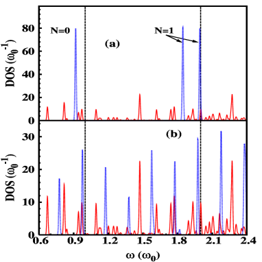
Figure 2: (Color online) (a) The time-averaged DOS of QD under THz field with $E=0.6$ kV/cm, $\Omega=4$ THz (red solid curve) and $E=0$ (blue dotted curve) for $\alpha_{R}=3\times 10^{-9}$ eV$\cdot$cm. (b) The time-averaged DOS of QD with Rashba SOC $\alpha_{R}=3\times 10^{-9}$ eV$\cdot$cm (red solid curve) and $\alpha_{R}=0$ (blue dotted curve) for $E=0.6$ kV/cm, $\Omega=4$ THz. The black dashed lines correspond to the positions of $\omega_{0}$ and $2\omega_{0}$.

In Fig. 2 we compare the time-averaged DOS with and without the SOC or the RF. The red (solid) curves are the DOS with both the SOC and the RF when $E=0.6$ kV/cm and $\Omega=4$ THz. The blue (dotted) curve in Fig. 2(a) is the DOS with only the SOC while the one in (b) is the DOS with only the RF. It is noted that in the figure the $\delta$-function $\delta(x)$ in the DOS is replaced by the Gaussian function $\exp(-x^{2}/2\sigma^{2})/(\sigma\sqrt{2\pi})$ with $\sigma=0.005\omega_{0}$. The DOS without the SOC and the RF peaks at $\omega=(N+1)\omega_{0}$ with value $(N+1)/(\sigma\sqrt{2\pi})(N=0,1,2,\cdots)$ (with the lowest two levels labelled by dashed lines in the figure). Each level has $(N+1)$-fold degeneracy as pointed out above. Nevertheless, by including only the SOC, the 2-fold degeneracy of $N=1$ major shell is lifted and the ground state energy ($N=0$) is lowered by $0.1\omega_{0}$, as indicated in Fig. 2(a). Moreover, including only the RF gives rise to many peaks at the integer multiplications of $\Omega$, as can be seen in Eq. (7). It is seen from Fig. 2(b) that these peaks are equidistant. The peaks are generally higher than those in the case with both the RF and the SOC, as the SOC causes additional splitting of the degenerate states.

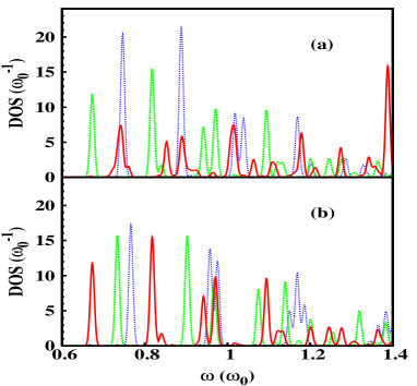
Figure 3: (Color online) The time-averaged DOS (a) for $E=0.5$ (green dot-dashed curve), 0.6 (blue dotted curve) and 0.7 (red solid curve) kV/cm, with $\alpha_{R}=3\times 10^{-9}$ eV$\cdot$cm and $\Omega=4$ THz and (b) for $\alpha_{R}=1$ (green dot-dashed curve), 2 (blue dotted curve) and 3 (red solid curve) $\times 10^{-9}$ eV$\cdot$cm, with $E=0.6$ kV/cm and $\Omega=4$ THz.

In order to further reveal the effect of the SOC and the RF on the system, we study the DOS under different RF and SOC. In Fig. 3, the DOS with different RF strengths (a) and Rashba coefficients (b) are plotted against energy. It is seen from Fig. 3(a) that the first peak of the DOS gets a red shift from $0.75\omega_{0}$ when $E=0.5$ kV/cm to $0.68\omega_{0}$ when $E=0.6$ kV/cm and then comes back to $0.74\omega_{0}$ when $E$ is further increased to $0.7$ kV/cm. This is a clear demonstration of the combined effect of the AC Stark effect and the DFKE.Nordstrom The AC Stark effect, which states that the energy difference becomes larger (smaller) if two energy levels are driven by an AC field with frequency below (above) the resonance.Nordstrom ; AH On the other hand, the DFKE states that the DOS has a blue-shift due to $E_{em}$ as indicated in Eq. (7).Jauho ; Jauho2 In the current case, the frequency of the THz irradiation is 4 THz, which is smaller than the resonant frequencies of the transitions from $N=0$ to $N=1$ major shells even when the SOC is included. Therefore there is an AC Stark effect which shift the $N=0$ major shell to red-side. This effect is responsible for the red shifts as the DOS in the low energy range mainly consists of $N=0$ major shell. Although both the DFKE blue-shift $E_{em}$ and the AC Stark red-shift increase with the RF strength, the AC Stark effect is more important at low RF strength, and it saturates at high RF strength where the blue-shift due to the DFKE dominates.Nordstrom Moreover, at low RF intensity the peaks locate at $\varepsilon_{\lambda}+E_{em}-n_{0}\Omega/2$ of a certain $n_{0}$ or replicas $\varepsilon_{\lambda}+E_{em}-(n_{0}+n)\Omega/2$ with small $n$’s. When the RF increases, the multi-photon processes become more and more important. As a result, the DOS becomes smoother as more and more multi-photon replicas appear. The effect of the SOC is plotted in Fig. 3(b), where the DOS under different Rashba coefficient $\alpha_{R}$ is plotted when the RF $E=0.6$ kV/cm and $\Omega=4$ THz. It is seen that the first peak shifts to the red side as $\alpha_{R}$ increases. This is understood as the SOC contributes to the AC Stark effect. From Eq. (5), one notices that the AC Stark effect enhances as the SOC is increased. Differing from the situation shown in Fig. 3(a), the blue shift $E_{em}$ from the DFKE does not change since the RF is fixed here. Therefore the shift of the first DOS peak is monotonic. Moreover, as $\alpha_{R}$ increases the multi-photon processes between different spin branches become more important and the DOS becomes smoother.

As said before, the DOSP is not zero when both the SOC and the RF are present. Due to the symmetry of the system, the only remaining spin polarization is along the $y$-axis. Consequently, the induced average magnetic moment can be calculated through the equationcheng_2005_APL

$${\bf M}(T)=\left(0,g\mu_{B}\int_{-\infty}^{E_{F}(T)}d\omega\ \mbox{Im}\rho_{\uparrow,\downarrow}(T,\omega),0\right)\ ,$$ (10)

where the time-dependent Fermi energy $E_{F}(T)$ is determined by $2\int_{-\infty}^{E_{F}(T)}d\omega\ \rho_{\uparrow,\uparrow}(T,\omega)=1$ when there is only one electron in the quantum dot. Due to the time periodicity introduced by the THz field, $E_{F}(T)$ and ${\bf M}(T)$ are also periodic functions of $T$ with period $T_{0}$. In Fig. 4, we plot the $y$-component of magnetic moment as a function of time. The magnetic moment is controlled by the RF strength, the frequency as well as the SOC and it can be qualitatively described by the factor $\Lambda$. The stronger the RF and the SOC are, the larger $\Lambda$ and $M_{y}$ become. On the other hand, the larger $\Omega$ is, the smaller $\Lambda$ becomes and therefore the smaller $M_{y}$ becomes.

Figure 4: The average magnetic moment $M_{y}$ versus the time for a single spin in QD at (a) $E=0.3$ (solid curve), 0.5 (dotted curve), and 0.6 (dot-dashed curve)  kV/cm for fixed $\Omega=4$ THz, and $\alpha_{R}=3\times 10^{-9}$ eV$\cdot$cm; (b) $\alpha_{R}=1$ (solid curve), 1.5 (dotted curve), and 3 (dot-dashed curve) $\times 10^{-9}$ eV$\cdot$cm for fixed RF with $\Omega=4$ THz and $E=0.6$ kV/cm; (c) $\Omega=4$ (solid curve), 4.6 (dotted curve), and 6 (dot-dashed curve)  THz for fixed $E=0.6$ kV/cm and $\alpha_{R}=3\times 10^{-9}$ eV$\cdot$cm .

In conclusion, we study the effects of the intense THz field on single electron spin in QD with the Rashba SOC. We calculate the single electron DOS at zero temperature and show that the DOS is greatly affected by the THz field and the SOC due to the dynamic Franz-Keldysh effect, the AC Stark effect and the side-band effect. It is shown that the joint effect of the THz field and the SOC can excite a THz magnetic moment which is controlled by the THz field strength, the THz frequency as well as the SOC. This provides a unique way to convert THz electric signals into THz magnetic ones which may be useful in full electrical magnetic resonance measurements.

This work was supported by the Natural Science Foundation of China under Grant Nos. 90303012 and 10574120, the Natural Science Foundation of Anhui Province under Grant No. 050460203, the Knowledge Innovation Project of Chinese Academy of Sciences and SRFDP. J.H.J. would like to thank J. L. Cheng for helpful discussions.

References

- (1) D. Loss and D. P. DiVincenzo, Phys. Rev. A 57, 120 (1998).
- (2) V. Cerletti, W. A. Coish, O. Gywat, and D. Loss, Nanotechnology 16, R27 (2005), and referrences there in.
- (3) H.-A. Engel, L. P. Kouwenhoven, D. Loss, and C. M. Marcus, Quantum Information Processing 3, 115 (2004), and reference there in.
- (4) V. N. Golovach, A. Khaetskii, and D. Loss, Phys. Rev. Lett. 93, 016601 (2004).
- (5) Semiconductor spintronics and quantum computation, ed. by D. D. Awschalom, D. Loss, and N. Samarth (Springer, Berlin, 2002).
- (6) I. Žutić, J. Fabian, and S. Das Sarma, Rev. Mod. Phys. 76, 323 (2004).
- (7) Y. Y. Wang and M. W. Wu, cond-mat/0601028.
- (8) J.M. Elzerman, R. Hanson, L.H. Willems van Beveren, B. Witkamp, L.M.K. Vandersypen, and L.P. Kouwenhoven, Nature 430, 431 (2004).
- (9) A. S. Bracker, E. A. Stinaff, D. Gammon, M. E. Ware, J. G. Tischler, A. Shabaev, Al. L. Efros, D. Park, D. Gershoni, V. L. Korenev, and I. A. Merkulov, Phys. Rev. Lett. 94, 047402 (2005).
- (10) M. Valín-Rodríguez, A. Puente, and L. Serra, Phys. Rev. B 66, 045317 (2002).
- (11) Y. Yacoby, Phys. Rev. 169, 610 (1968).
- (12) A. P. Jauho and K. Johnsen, Phys. Rev. Lett. 76, 4576 (1996).
- (13) K. Johnsen and A.-P. Jauho, Phys. Rev. B. 57, 8860 (1998).
- (14) K. B. Nordstrom, K. Johnsen, S. J. Allen, A. -P. Jauho, B. Birnir, J. Kono, and T. Noda, Phys. Rev. Lett. 81, 457 (1998).
- (15) A. H. Rodriguez, L. Meza-Montes, C. Trallero-Giner, and S. E. Ulloa, phys. stat. sol. (b) 242, 1820 (2005).
- (16) J. Cerne, K. Kono, T. Inoshita, M. Sundaram, and A. C. Gossard, Appl. Phys. Lett. 70, 3543 (1997).
- (17) J. Kono, M. Y. Su, T. Inoshita, T. Noda, M. S. Sherwin, S. J. Allen, Jr., and H. Sakaki, Phys. Rev. Lett. 79, 1758 (1997).
- (18) C. Phillips, M. Y. Su, M. S. Sherwin, J. Ko, and L. Coldren, Appl. Phys. Lett. 75, 2728 (1999).
- (19) M. Grifoni and P. Hänggi, Phys. Rep. 304, 229, and reference there in.
- (20) S. Kohler, J. Lehmann, and P. Hänggi, Phys. Rep. 406, 379, and reference there in.
- (21) L. Arrachea, Phys. Rev. B 72, 125349 (2005) , and reference there in.
- (22) J. L. Cheng and M. W. Wu, Appl. Phys. Lett. 86, 032107 (2005).
- (23) C. M. Wang, S. Y. Liu, and X. L. Lei, Phys. Rev. B. 73, 035333 (2006).
- (24) Y. A. Bychkov and E. Rashba, Sov. Phys. JETP Lett. 39, 78 (1984).
- (25) R. Winkler, Spin-Orbit Coupling Effects in Two-Dimensional Electron and Hole Systems (Springer, Berlin, 2003).
- (26) G. Dresselhaus, Phys. Rev. 100, 580 (1955).
- (27) D. Grundler, Phys. Rev. Lett. 26, 6074 (2000).
- (28) Y. Sato, T. Kita, S. Gozu, and S. Yamada, J. Appl. Phys. 89, 8017 (2001).
- (29) J. H. Shirley, Phys. Rev. 138, B979 (1965).
- (30) J. L. Cheng, M. W. Wu, and C. Lü, Phys. Rev. B 69, 115318 (2004).
- (31) R. Hanson, B. Witkamp, L. M. K. Vandersypen, L. H. Willems van Beveren, J. M. Elzerman, and L. P. Kouwenhoven, Phys. Rev. Lett. 91, 196802 (2003).