Nonequilibrium dynamic exponent and spin-glass transitions

Abstract

Nonequilibrium dynamics of the $\pm J$ Ising, the XY, and the Heisenberg spin-glass models are investigated in three dimensions. A nonequilibrium dynamic exponent is calculated from the dynamic correlation length. The spin-glass dynamic exponent continuously depends on the temperature. There is no anomaly at the critical temperature as is recently reported by Katzgraber and Campbell. On the other hand, the chiral-glass dynamic exponent takes a constant value above the spin-glass transition temperature ($T_{\mathrm{sg}}$), and becomes temperature-dependent below $T_{\mathrm{sg}}$. The finite-time scaling analyses on the spin- and the chiral-glass susceptibility are performed using the temperature dependence of the dynamic exponent. The critical temperature and the critical exponents are estimated with high precisions. In the Ising model, $T_{\mathrm{sg}}=1.18(2)$, $\nu_{\mathrm{sg}}=1.75(10)$, $\gamma_{\mathrm{sg}}=3.4(2)$, and $z_{\mathrm{sg}}=5.1(1)$. In the XY model, $T_{\mathrm{sg}}=0.435(15)$, $\nu_{\mathrm{sg}}=1.25(15)$, $\gamma_{\mathrm{sg}}=2.30(25)$, and $z_{\mathrm{sg}}=5.0(1)$ for the spin-glass transition, and $T_{\mathrm{cg}}=0.445(15)$, $\nu_{\mathrm{cg}}=1.05(10)$, $\gamma_{\mathrm{cg}}=1.65(20)$, and $z_{\mathrm{cg}}=5.1(2)$ for the chiral-glass transition. In the Heisenberg model, $T_{\mathrm{sg}}=0.18(1)$, $\nu_{\mathrm{sg}}=1.55(15)$, $\gamma_{\mathrm{sg}}=2.9(2)$, and $z_{\mathrm{sg}}=5.1(1)$ for the spin-glass transition, and $T_{\mathrm{cg}}=0.23(1)$, $\nu_{\mathrm{cg}}=0.70(15)$, $\gamma_{\mathrm{cg}}=0.65(15)$, and $z_{\mathrm{cg}}=5.0(2)$ for the chiral-glass transition. A difference of the spin- and the chiral-glass transition temperatures is resolved in the Heisenberg model. The dynamic critical exponent takes almost the same value for all transitions. It suggests that the spin-glass and the chiral-glass transitions in three dimensions are dynamically universal.

I Introduction

Randomness and frustration produce nontrivial phenomena in spin glassesSGReview1 ; SGReview2 ; SGReview3 . There is no spatial order in the spin-glass phase. The spins are ordered only in the time direction: spins randomly freeze below the critical temperature. Growth of the spin-glass correlations is very slow. Most of interesting observations in experiments and in computer simulations are essentially nonequilibrium phenomena. Aging, memory and rejuvenation effects are the typical examples.dupuis1 ; jonsson1 ; bouchaud1 ; bert1 It has become clear that a domain size of frozen spins plays an important role in explaining these phenomena.fisherhuse ; bouchaud2 ; yoshino1 ; berthier1 ; scheffler ; yoshino2 ; parisi1 ; kisker1 ; komori1 ; berthier2 ; dupuis2 ; jonsson2 ; yoshino3 ; nakamura3 ; berthier3 ; katzgraber Details of time evolution of the domain size may determine the dynamics of spin glasses.

In the second-order phase transitions, a correlation length $\xi$ and a correlation time $\tau$ diverge at the critical temperature. The dynamic scaling relation holds as $\tau\sim\xi^{z}$ with the dynamic critical exponent $z$. If we observe the correlation length as a function of time, it also diverges algebraically with the same exponent. It is written as $\xi(t)\sim t^{1/z}.$ Consequently, the magnetic susceptibility $\chi(t)$ diverges with an exponent $\gamma/z\nu$.

The dynamic scaling relation also holds in spin glasses at the critical temperature. Husehuse remarked that a time evolution of the spin-glass susceptibility $\chi_{\mathrm{sg}}(t)$ diverges algebraically with an exponent $\gamma/z\nu$ in the Ising spin-glass model. Blundell et al.blundell found that a relaxation function of the Binder parameter $g_{\mathrm{sg}}$ also diverges with an exponent $1/z$. The spin-glass correlation length is also considered to diverge algebraically at the critical temperature.

Below the spin-glass transition temperature, $T_{\mathrm{sg}}$, the algebraic divergence of the spin-glass correlation length is considered to continue in the nonequilibrium process. An exponent of the divergence linearly depends on the temperature:berthier2 ; parisi1 ; kisker1 ; komori1 ; yoshino3 ; nakamura3

$$\frac{1}{z_{\mathrm{s}}(T)}=\frac{T}{z_{\mathrm{sg}}T_{\mathrm{sg}}}.$$ (1)

Here, we call $z_{\mathrm{s}}(T)$ a spin-glass nonequilibrium dynamic exponent. It is defined only in the nonequilibrium relaxation process. It equals to the dynamic critical exponent of the spin glass transition, $z_{\mathrm{sg}}$, at the critical temperature.

Recently, Katzgraber and Campbell katzgraber remarked that the relation (1) continues to hold above $T_{\mathrm{sg}}$, and that there is no anomaly at the critical temperature. The model they investigated is the Gaussian-bond Ising spin-glass model and the gauge-glass model in three and four dimensions. It is very important whether or not this finding is common to various spin-glass models. In regular systems, the dynamic critical exponent $z$ governs the algebraic growth of the correlation length in the nonequilibrium relaxation process above the critical temperature. The temperature dependence of $z$ above $T_{\mathrm{sg}}$ is out of our assumption regarding the dynamics of spin glasses.

The dynamic scaling relation in the nonequilibrium relaxation process of the spin-glass models suggests that we can study the spin-glass phase transition using the nonequilibrium relaxation method.Stauffer ; Ito ; ItoOz1 ; OzIto2 It is a powerful tool to estimate the critical temperature and the critical exponent with high precisions. It has been applied to slow dynamic systems with frustration and/or randomness.OzIto2 ; shirahata1 ; nakamura ; nakamura2 ; shirahata2 ; yamamoto1 ; nakamura3 ; nakamura4 A key concept of the method is an exchange of time and size by the dynamic scaling relation, $t\rightleftarrows L^{z}$. Here, a single exponent $z$ is considered to satisfy the relation above the critical temperature. This assumption may be broken by the relation (1). Therefore, we must reconsider the nonequilibrium relaxation analysis in the spin-glass problems taking into account the relation (1). Then, the finite-time-scaling results may be influenced.

In this paper we carry out extensive Monte Carlo simulations. It is made clear that the relation (1) is satisfied for the spin-glass transitions in all models. It continues regardless the critical temperature without anomaly. On the other hand, the temperature dependence of the nonequilibrium dynamic exponent of the chiral-glass correlation length only appears below $T_{\mathrm{sg}}$. It takes a constant value above $T_{\mathrm{sg}}$ as in the regular systems. The finite-time scaling analyses are performed using the temperature dependence of the dynamic exponent. The transition temperature and the critical exponents are estimated with higher precisions compared to our previous results. We give a conclusion to a problem of whether or not the spin- and the chiral-glass transitions occur simultaneously in the XY and the Heisenberg models.

The present paper is organized as follows. Section II describes a model and physical quantities we observe in simulations. Section III explains our numerical method and some technical details. Results of the Ising, the XY, and the Heisenberg models are presented in Sec. IV, V, and VI, respectively. Section VII is devoted to summary and discussions.

II Model and Observables

II.1 Model

We study the $\pm J$ spin-glass model in a simple cubic lattice.

$${\cal H}=-\sum_{\langle ij\rangle}J_{ij}\mbox{\boldmath$S$}_{i}\cdot\mbox{\boldmath$S$}_{j}$$ (2)

The sum runs over all the nearest-neighbor spin pairs $\langle ij\rangle$. The interactions, $J_{ij}$, take the two values $+J$ and $-J$ with the same probability. The temperature, $T$, is scaled by $J$. Linear lattice size is denoted by $L$. A total number of spins is $N=L\times L\times(L+1)$, and skewed periodic boundary conditions are imposed. The spins are updated by the single-spin-flip algorithm using the conventional Metropolis probability. We treat three types of spin dimensions: the Ising model with $\mbox{\boldmath$S$}_{i}=S_{iz}$, the XY model with $\mbox{\boldmath$S$}_{i}=(S_{ix},S_{iy})$, and the Heisenberg model with $\mbox{\boldmath$S$}_{i}=(S_{ix},S_{iy},S_{iz})$. In the XY model, each spin is defined by an angle in the XY plane: $\mbox{\boldmath$S$}_{i}=(\cos\theta_{i},\sin\theta_{i})$. The angle $\theta_{i}$ takes continuous values in $[0,2\pi)$; however, we divide the interval into 1024 discrete states in this study. The effect of the discretization is checked by comparing data of 1024-state simulations with those of 2048-state simulations. It is found to be negligible.

The physical quantities that are calculated in our simulations are the spin-glass susceptibility, $\chi_{\mathrm{sg}}$, the chiral-glass susceptibility, $\chi_{\mathrm{cg}}$, and the spin- and the chiral-glass correlation functions, $f_{\mathrm{sg}}$ and $f_{\mathrm{cg}}$, from which we estimate the correlation lengths, $\xi_{\mathrm{sg}}$ and $\xi_{\mathrm{cg}}$.

II.2 Spin-glass susceptibility

The spin-glass susceptibility is defined by the following expression.

$$\chi_{\mathrm{sg}}\equiv\frac{1}{N}\left[\sum_{i,j}\langle\mbox{\boldmath$S$}_{i}\cdot\mbox{\boldmath$S$}_{j}\rangle^{2}\right]_{\mathrm{c}}$$ (3)

The thermal average is denoted by $\langle\cdots\rangle$, and the random-bond configurational average is denoted by $[\cdots]_{\mathrm{c}}$. The thermal average is replaced by an average over independent real replicas that consist of different thermal ensembles:

$$\langle\mbox{\boldmath$S$}_{i}\cdot\mbox{\boldmath$S$}_{j}\rangle=\frac{1}{m}\sum_{A=1}^{m}\mbox{\boldmath$S$}_{i}^{(A)}\cdot\mbox{\boldmath$S$}_{j}^{(A)}.$$ (4)

A replica number is denoted by $m$. The superscripts $A$ is the replica index. We prepare $m$ real replicas for each random bond with different initial spin configurations. Each replica is updated using a different random number sequence. The thermal average is taken only by this replica average in our numerical scheme. A replica number controls an accuracy of the thermal average.

An overlap between two replicas, $A$ and $B$, is defined by

$$q_{\mu\nu}^{AB}\equiv\frac{1}{N}\sum_{i}{S}_{i\mu}^{(A)}{S}_{i\nu}^{(B)}.$$ (5)

Here, subscripts $\mu$ and $\nu$ represent three spin directions $x,y$, and $z$. The spin-glass susceptibility is estimated using the overlap function:

$$\chi_{\mathrm{sg}}=\frac{2N}{m(m-1)}\left[\sum_{A>B,\mu,\nu}\langle(q^{AB}_{\mu\nu})^{2}\rangle\right]_{\mathrm{c}}.$$ (6)

Similarly, the chiral-glass susceptibility in the XY model KawamuraXY1 ; KawamuraXY2 ; KawamuraXY3 is defined by

$$\chi_{\mathrm{cg}}\equiv\frac{6N}{m(m-1)}\left[\sum_{A>B}(q_{\kappa}^{AB})^{2}\right]_{\mathrm{c}},$$ (7)

where

$$q_{\kappa}^{AB} \equiv \frac{1}{3N}\sum_{\alpha}\,{\kappa}_{\alpha}^{(A)}{\kappa}_{\alpha}^{(B)},$$ (8)

$$\kappa_{\alpha}^{(A)} \equiv \frac{1}{2\sqrt{2}}\sum_{\langle jk\rangle\in\alpha}J_{jk}\sin{(\theta_{j}^{(A)}-\theta_{k}^{(A)})}.$$ (9)

A local chirality variable, $\kappa_{\alpha}^{(A)}$, is the $z$ component of the vector chirality. It is defined at each square plaquette, $\alpha$, that consists of the nearest-neighbor bonds, $\langle jk\rangle$. In the Heisenberg model, we use the scalar chiralityKawamuraH1 ; HukushimaH ; HukushimaH2 , which is defined by

$$\kappa_{i,\mu}^{(A)}\equiv\mbox{\boldmath$S$}_{i+\hat{\mbox{\boldmath$e$}}_{\mu}}^{(A)}\cdot(\mbox{\boldmath$S$}_{i}^{(A)}\times\mbox{\boldmath$S$}_{i-\hat{\mbox{\boldmath$e$}}_{\mu}}^{(A)}),$$ (10)

where $\hat{\mbox{\boldmath$e$}}_{\mu}$ denotes a unit lattice vector along the $\mu$ axis. The overlap function and the chiral-glass susceptibility are defined in the same manner as in the XY model.

II.3 Dynamic correlation length

A spin-glass correlation function is defined by the following expression (11).

$$f_{\mathrm{sg}}(r) \equiv \left[\sum_{i}^{N}\langle\mbox{\boldmath$S$}_{i}\cdot\mbox{\boldmath$S$}_{i+r}\rangle^{2}\right]_{\mathrm{c}}$$ (11)

$$= \left[\frac{2}{m(m-1)}\sum_{A>B,i,\mu\nu}q_{\mu\nu}^{AB}(i)q_{\mu\nu}^{AB}(i+r)\right]_{\mathrm{c}}$$ (12)

$$= \left[\sum_{i}^{N}\left(\frac{1}{m}\sum_{A}^{m}\mbox{\boldmath$S$}_{i}^{(A)}\cdot\mbox{\boldmath$S$}_{i+r}^{(A)}\right)^{2}\right]_{\mathrm{c}}$$ (13)

Here, $q_{\mu\nu}^{AB}(i)=S_{i\mu}^{(A)}S_{i\nu}^{(B)}$ is the spin overlap on the $i$th site. When a replica number is two, it is equivalent to the four-point correlation function as is shown in Eq. (12). Since $m$ is large in this study, it is very time-consuming to take an average over $m(m-1)/2$ different overlap functions. Therefore, we use another expression (13) for $f_{\mathrm{sg}}(r)$. For a given distance $r$ and a site $i$, we calculate a spin correlation function for replica $A$, and store it in a memory array. Then, the replica average is taken and the obtained value is squared. Taking a summation of the squared value over lattice sites $i$ we obtain the correlation function $f_{\mathrm{sg}}(r)$ for a given distance $r$. Changing a value of $r$ we do the same procedure to evaluate $f_{\mathrm{sg}}(r)$. Total amount of calculation is much smaller in this procedure because the maximum value of $r=L/2$ is much smaller than $m(m-1)/2$.

We obtain a chiral-glass correlation function in the same manner replacing the local spin variables with the local chirality variables. Here, we only consider correlations between two parallel square plaquettes in the XY model. A pair of three neighboring spins in the same direction is considered in the Heisenberg model. We estimate the spin- and the chiral-glass correlation lengths, $\xi_{\mathrm{sg}}$ and $\xi_{\mathrm{cg}}$, from the correlation functions using the following expression.

$$f_{\mathrm{sg/cg}}(r)=f_{0}\exp\left(-\frac{r}{\xi_{\mathrm{sg/cg}}}\right)$$ (14)

A problem in this expression is a prefactor $f_{0}$. We may suppose several forms for $f_{0}$. For example, $f_{0}\sim l^{2-d-\eta}$. However, the obtained value may depend on a value of $\eta$, which is not known yet. Therefore, we take a rather brute-force approach as explained below. Then, the relaxation functions of the correlation length, $\xi_{\mathrm{sg}}$ and $\xi_{\mathrm{cg}}$, are obtained. This is sometimes called the dynamic correlation length.

We prepare a sufficiently large lattice and calculate the correlation functions with high precisions, typically up to an order of $10^{-6}$. The correlation functions asymptotically exhibit a single exponential decay when $r$ is large enough. We estimate the correlation length using data in this asymptotic region. Figure 1 shows the lin-log plot of $f_{\mathrm{sg}}(r)$ and $f_{\mathrm{cg}}(r)$ in the Ising and the Heisenberg models near the critical temperature. Linearity is good when the distance is larger than a typical distance, $r_{\mathrm{min}}$. This behavior guarantees our single-exponential fitting when estimating the correlation lengths. Values of $r_{\mathrm{min}}$ are summarized in Sec. III.5.

Correlation functions sometimes exhibit bending to convergence as shown in Fig. 1(b). It is considered to be an outcome of the boundary effect. Since we work with the skewed periodic boundary conditions, the farthest distance is $L/2$. The correlation data near $r=L/2=29$ are influenced by the boundary conditions. Therefore, the spin-glass data when $r>25$ show convergence. We cut off such data when we estimate the correlation length. We also cut off data which fluctuate from the fitting line. The minimum distance and the cut-off distance are determined so that the relative deviations of data from the fitting line stay within 5%. Arrows in Fig. 1 depict the cut-off distance.

It is also noted that the chiral-glass correlation functions are smaller than the spin-glass ones by three digits. Estimations of the chiral-glass correlation length are usually very difficult, and the error bars become relatively large.

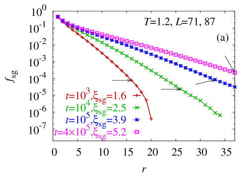
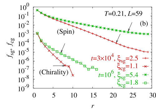
Figure 1: (Color online) Spin- and chiral-glass correlation functions are plotted versus distance $r$ at various time step $t$. (a) Results of the Ising model. The temperature $T=1.2$ is near the critical point. The lattice size $L=71$ for $t=10^{3}$ and $L=87$ for $t\geq 10^{4}$. (b) Results of the Heisenberg model. The temperature $T=0.21$ is near the chiral-glass transition temperature. The lattice size $L=59$. Arrows depict a cut-off distance when estimating the correlation length.

III Method

III.1 Nonequilibrium relaxation method

We start the simulations with random spin configurations, which is a paramagnetic state at $T=\infty$. The temperature is quenched to a finite value at the first Monte Carlo step. We calculate the physical observables at each observation time, and obtain the relaxation functions. Changing the initial spin state, the random bond configuration, and the random number sequence, we start another simulation to obtain another set of the relaxation functions. We calculate the average of the relaxation functions over these independent Monte Carlo simulations.

It is necessary to check a time scale when the finite-size effects appear in the relaxation functions. We must stop the simulations before the size effects appear. The nonequilibrium relaxation method is based upon taking the infinite-size limit before the equilibrium limit is taken. Data presented in this paper can be regarded as those of the infinite-size system.

III.2 Finite-time scaling analysis

We estimate the transition temperature using the finite-time-scaling analysis.OzIto2 This is a direct interpretation of the conventional finite-size-scaling analysis considering the dynamic scaling hypothesis: $\tau\sim\xi^{z}$. Through this relation, the “size” is replaced by the “time.” Here, the temperature dependence of the nonequilibrium dynamic exponent, $z_{\mathrm{s}}(T)$, written in Eq. (1) should be taken into account. The temperature coefficient, $1/z_{\mathrm{sg}}T_{\mathrm{sg}}$, is obtained beforehand by the scaling analysis of the dynamic correlation length. The following equation represents the scaling formula for the spin-glass susceptibility.

$$\chi_{\mathrm{sg}}(t)t^{-\gamma_{\mathrm{sg}}/z_{\mathrm{s}}(T)\nu_{\mathrm{sg}}}=\tilde{\chi}_{\mathrm{sg}}(t/(T-T_{\mathrm{sg}})^{-z_{\mathrm{s}}(T)\nu_{\mathrm{sg}}})$$ (15)

Here, $\tilde{\chi}$ denotes a universal scaling function. We plot data of the spin-glass susceptibility multiplied by $t^{-\gamma_{\mathrm{sg}}/z_{\mathrm{s}}(T)\nu_{\mathrm{sg}}}$ against $t/(T-T_{\mathrm{sg}})^{-z_{\mathrm{s}}(T)\nu_{\mathrm{sg}}}$. We choose scaling parameters, $T_{\mathrm{sg}}$, $\gamma_{\mathrm{sg}}$, and $\nu_{\mathrm{sg}}$ so that they yield the best universal scaling function.

We perform a scaling analysis using a criterion which we proposed in the previous paper.yamamoto1 In general, it is difficult to choose proper scaling parameters because the universal scaling function form is not known. One usually approximate the scaled data by some polynomial functions, and choose scaling parameters so that the fitting error becomes smallest. However, if we change the scaling parameter, the function form itself changes. Then, a significance of the fitting error changes. A value of the fitting error sometimes misleads us to incorrect results. Therefore, we take another strategy.

Since the correct scaling function is universal, it is free from human factors. It should be robust against a change of a temperature range of data we use in the analysis; it should be robust against a change of discarding steps in simulations; it should be robust against a change of procedures determining scaling parameters. In this paper, we consider the following three procedures:

• (Procedure-1) For a given value of $\gamma_{\mathrm{sg}}/\nu_{\mathrm{sg}}$, search $T_{\mathrm{sg}}$ and $\nu_{\mathrm{sg}}$ that yield the smallest fitting error.

• (Procedure-2) For a given value of $\gamma_{\mathrm{sg}}$, search $T_{\mathrm{sg}}$ and $\nu_{\mathrm{sg}}$ that yield the smallest fitting error.

• (Procedure-3) For a given value of $\nu_{\mathrm{sg}}$, search $T_{\mathrm{sg}}$ and $\gamma_{\mathrm{sg}}$ that yield the smallest fitting error.

Here, we mean the smallest fitting error by the least-square deviations when we approximate the scaled data with a polynomial function of seven orders. We also change the temperature range and a number of discarding steps for each procedure. Scaling results systematically depend on these procedures. The most probable result is obtained by a crossing intersection or a merging point because it should be independent of the procedures. An error bar of the result is given by a range of scaling parameters which yield a good scaling plot.

III.3 Replica number VS Sample number

A replica number controls an accuracy of the thermal average. A sample number controls an accuracy of the configurational average. In order to improve an accuracy of the thermal average, $m$ should be large. However, if we set it large, a sample number is restricted, which causes a poor configurational average. So, there is a question. In order to improve an accuracy of the final results, which number should be set large first, a replica number $m$ or a sample number $N_{\mathrm{s}}$? Most of the simulational studies in spin glasses take a choice of $m=2$.

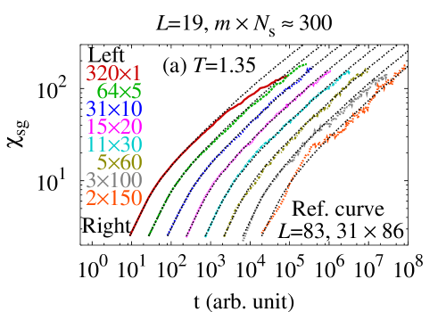
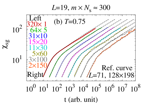
Figure 2: (Color online) Relaxation functions of the spin-glass susceptibility of the Ising model when a replica number $m$ and a bond sample number $N_{\mathrm{s}}$ are changed keeping the product almost constant, $m\times N_{\mathrm{s}}\sim 300$. (a) $T=1.35>T_{\mathrm{c}}$, and (b) $T=0.75<T_{\mathrm{c}}$. Reference curves are plotted with black dotted line, which are obtained by (a) $L=83$, $m=31$, and $N_{\mathrm{s}}=86$; (b) $L=71$, $m=128$, and $N_{\mathrm{s}}=198$. Each function is shifted to the $t$ direction in order to compare the deviations.

Figure 2 shows the answer. Relaxation functions of the spin-glass susceptibility in the Ising model are plotted both in the paramagnetic phase(a) and in the spin-glass phase(b). A product $m\times N_{\mathrm{s}}$ is set almost equal to 300 and the lattice size is set to $L=19$. A total number of spin updates and a total computational time are same. We also plot a reference curve which is obtained by a sufficiently large simulation. All relaxation curves of $L=19$ are consistent with the reference curves. Statistical fluctuations are large when the replica number is small. They are suppressed as we increase a replica number and decrease a sample number. However, when a sample number is one, there is a systematic deviation from the reference curve. This deviation depends on each random-bond sample. The dependence becomes small and the deviation appears later if we increase the lattice size. A sample number can be set small in the nonequilibrium process of a sufficiently large system, where the size can be considered as infinity. Therefore, a replica number should be set larger first when the total computational time is restricted. We need at least several sample numbers to avoid systematic deviation due to the sample dependence. The statement is true both in the paramagnetic phase and in the spin-glass phase.

In this study, we set $m=128$ and $m=192$ for the Ising model, $m=32$ and $m=64$ for the XY model, and $m=32$ for the Heisenberg model. Simulation conditions are summarized in Sec. III.5.

III.4 Updating probability: Metropolis VS Heat-bath

Spin update dynamics in this paper is the Metropolis algorithm. A heat-bath algorithm Olive is usually adopted in a simulation of the Heisenberg model. However, we found a chaotic behavior in a nonequilibrium dynamics of the heat-bath algorithm as shown in Fig. 3.

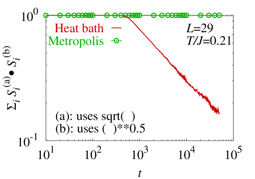
Figure 3: (Color online) A replica overlap in the Heisenberg model between the exactly same replica with the same random number sequence but with a different usage of a square-root function. Replica (a) uses a built-in sqrt function, and replica (b) uses an exponential function. A heat-bath algorithm and a Metropolis algorithm are compared. A temperature, $T/J=0.21$, is near the chiral-glass transition point.

We prepare two real replicas, (a) and (b), with the same bond configurations with the same initial spin configurations with the same random number sequence. Only one difference is a use of a square-root function. A replica-(a) uses a built-in sqrt(x) function for $\sqrt{x}$, while a replica-(b) uses an exponential function x**0.5. An spin overlap function between two replicas is observed. Mathematically, it must stay unity forever. However, the overlap decays after some characteristic time in the heat-bath algorithm. This time depends on the temperature and also a compiler option which controls numerical precisions. It becomes longer for higher precisions. To the contrary, an overlap in the Metropolis algorithm stays unity.

Mathematical functions are numerically approximated in computer calculations. A square-root function, $\sqrt{x}$, is one of the most difficult function to approximate. The error is negligible for each function call. However, successive calls may enlarge the error. In the heat-bath algorithm,Olive a spin state, $\mbox{\boldmath$S$}_{i}$, is a function of a local molecular field from the neighboring spins, $\mbox{\boldmath$S$}_{j}$. The neighboring spin state, $\mbox{\boldmath$S$}_{j}$, is also a function of the molecular field which contains $\mbox{\boldmath$S$}_{i}$. Therefore, a spin state $\mbox{\boldmath$S$}_{i}$ given by a complex function of spin states of itself and neighboring spins in the past. A square-root function is called successively in this procedure. Therefore, a small numerical error may be enhanced. A spin state may become different from the correct one. We cannot know which state is correct because every computer simulation contains a numerical error.

In the Metropolis algorithm, each spin state is generated independently by random numbers. There is no correlation between spin-state candidates in a time sequence. The overlap in Fig. 3 stays unity as mathematically required. In this paper, we study a spin-chirality separation in the Heisenberg model. The separation may be observed in a very narrow temperature range. We deal with this very naive problem by the relaxation method. Therefore, we use a Metropolis algorithm in order to exclude out the unphysical chaotic behavior from the relaxation process.

III.5 Simulation conditions

In this subsection, we summarize simulation conditions in Tabs. 2, 2, 3, 4, and 5. A sample number $N_{\mathrm{s}}$, a linear size $L$, a minimum distance of the spin correlations $r_{\mathrm{min}}$ vary with a Monte Carlo time step. Numbers above right arrows in tables denote a time step when the condition changes.

In the Ising model, a replica number is 128 except for a case of $T=1.4$ and $L=111$, where it is 192. Simulation conditions when the dynamic correlation length is estimated are listed in Tab. 2, and those when the spin-glass susceptibility is calculated are listed in Tab. 2.

$T$	$L$	$r_{\mathrm{min}}$	$N_{\mathrm{s}}$
1.7	71	7	98
1.6	71 $\longrightarrow^{2\cdot 10^{3}}$ 87	7 $\longrightarrow^{2\cdot 10^{3}}$ 12	659 $\longrightarrow^{5\cdot 10^{3}}$ 651
1.5	71 $\longrightarrow^{10^{4}}$ 95	10 $\longrightarrow^{10^{4}}$ 16	309 $\longrightarrow^{500}$ 95 $\longrightarrow^{10^{4}}$ 338
1.4	71 $\longrightarrow^{5\cdot 10^{4}}$ 111	10 $\longrightarrow^{5\cdot 10^{4}}$ 16	426 $\longrightarrow^{5000}$ 232 $\longrightarrow^{5\cdot 10^{4}}$ 25
1.3	71 $\longrightarrow^{10^{4}}$ 87	10 $\longrightarrow^{10^{4}}$ 16	112 $\longrightarrow^{10^{4}}$ 48
1.2	71 $\longrightarrow^{10^{4}}$ 87	10 $\longrightarrow^{10^{4}}$ 14	236 $\longrightarrow^{10^{4}}$ 163 $\longrightarrow^{5\cdot 10^{4}}$ 85 $\longrightarrow^{10^{5}}$ 45
1.0	71	10	195 $\longrightarrow^{10^{4}}$ 65
0.75	71	8	198 $\longrightarrow^{10^{4}}$ 65

Table 1: Simulation conditions of the Ising model when $\xi_{\mathrm{sg}}$ is estimated. Numbers above right arrows denote a time step when the value changes.

$T$	$L$	$N_{\mathrm{s}}$	$T$	$L$	$N_{\mathrm{s}}$
1.54	43	2321	1.44	55	1017
1.5	43	2078	1.425	59	1101
1.475	43	2208	1.42	59	1288
1.46	43	1930	1.4	59	809
1.45	43	1874	1.375	71	412

$T$	$L$	$N_{\mathrm{s}}$
1.35	83	388 $\longrightarrow^{3\cdot 10^{5}}$ 164
1.338	83	351 $\longrightarrow^{3\cdot 10^{5}}$ 150
1.325	83	306 $\longrightarrow^{3\cdot 10^{5}}$ 214
1.3125	91	458 $\longrightarrow^{2\cdot 10^{5}}$ 409 $\longrightarrow^{5\cdot 10^{5}}$ 340 $\longrightarrow^{9\cdot 10^{5}}$ 134
1.3	83	130

Table 2: Simulation conditions of the Ising model when $\chi_{\mathrm{sg}}$ is calculated. Numbers above right arrows denote a time step when the value changes.

$T$	$L$	$N_{\mathrm{s}}$
0.6	39	219 $\longrightarrow^{10^{3}}$ 624 $\longrightarrow^{3\cdot 10^{4}}$ 405
0.55	55	1833 $\longrightarrow^{10^{3}}$ 174
0.5	55	247 $\longrightarrow^{5\cdot 10^{4}}$ 99
0.45	55	2056 $\longrightarrow^{10^{3}}$ 675 $\longrightarrow^{3\cdot 10^{4}}$ 308
0.43	55	167 $\longrightarrow^{10^{5}}$ 76
0.41	55	241
0.375	45 $\longrightarrow^{10^{5}}$ 55	440 $\longrightarrow^{3\cdot 10^{4}}$ 191 $\longrightarrow^{10^{5}}$ 26

Table 3: Simulation conditions of the XY model when $\xi_{\mathrm{sg/cg}}$ is estimated. Numbers above right arrows denote a time step when the value changes.

$T$	$L$	$N_{\mathrm{s}}$	$T$	$L$	$N_{\mathrm{s}}$
0.62	39	128	0.50	39	485 $\longrightarrow^{10^{5}}$ 42
0.6	39	415	0.49	55	32
0.56	39	190	0.48	55	143 $\longrightarrow^{10^{5}}$ 30
0.54	39	426	0.47	55	101 $\longrightarrow^{10^{5}}$ 54
0.53	39	402	0.45	55	675 $\longrightarrow^{3\cdot 10^{4}}$ 308
0.52	39	289 $\longrightarrow^{10^{5}}$ 78	0.43	55	167 $\longrightarrow^{10^{5}}$ 76
0.51	39	351

Table 4: Simulation conditions of the XY model when $\chi_{\mathrm{sg/cg}}$ are calculated. Numbers above right arrows denote a time step when the value changes.

$T$	$L$	$r_{\mathrm{min}}^{\mathrm{sg}}$	$r_{\mathrm{min}}^{\mathrm{cg}}$	$N_{\mathrm{s}}$
0.29	59			158 $\longrightarrow^{10^{4}}$ 112 $\longrightarrow^{5\cdot 10^{4}}$ 103
0.28	59			174 $\longrightarrow^{10^{4}}$ 81
0.275	59			116
0.27	59	10	4	200 $\longrightarrow^{2\cdot 10^{4}}$ 98
0.265	59			172
0.26	59			249 $\longrightarrow^{2\cdot 10^{4}}$ 177 $\longrightarrow^{10^{5}}$ 51
0.255	59			103
0.25	59		5	213 $\longrightarrow^{10^{4}}$ 147 $\longrightarrow^{10^{5}}$ 56
0.245	59			135 $\longrightarrow^{10^{5}}$ 58
0.24	59	10	5	121 $\longrightarrow^{10^{5}}$ 72
0.238	59	10	5	99
0.23	59	10	5	162 $\longrightarrow^{10^{4}}$ 67
0.225	59	10	5	185 $\longrightarrow^{10^{4}}$ 61
0.22	59	10	5	110 $\longrightarrow^{2\cdot 10^{4}}$ 86
0.215	59	10	5	185 $\longrightarrow^{10^{4}}$ 67 $\longrightarrow^{10^{5}}$ 18 $\longrightarrow^{3\cdot 10^{5}}$ 8
0.21	75 $\longrightarrow^{2\cdot 10^{4}}$ 59	10	5	86 $\longrightarrow^{2\cdot 10^{4}}$ 124 $\longrightarrow^{10^{5}}$ 88 $\longrightarrow^{5\cdot 10^{5}}$ 26
0.207–0.1925	59			16
0.18	59	10	5	182 $\longrightarrow^{2\cdot 10^{4}}$ 121 $\longrightarrow^{10^{5}}$ 17
0.15	59	8	5	279 $\longrightarrow^{5\cdot 10^{4}}$ 138 $\longrightarrow^{10^{5}}$ 18
0.1	75 $\longrightarrow^{10^{5}}$ 59	8	5	24 $\longrightarrow^{10^{5}}$ 10

Table 5: Simulation conditions of the Heisenberg model. Numbers above right arrows denote a time step when the value changes.

In the XY model, a replica number is 64 when the dynamic correlation length is estimated, and it is 32 when the susceptibility is estimated. The minimum distance when estimating the correlation length is $r_{\mathrm{min}}^{\mathrm{sg}}=8$ for the spin glass and $r_{\mathrm{min}}^{\mathrm{cg}}=5$ for the chiral glass. Simulation conditions when the dynamic correlation length is estimated are listed in Tab. 3, and those when the spin-glass susceptibility is calculated are listed in Tab. 4.

In the Heisenberg model, a replica number is 32. Simulation conditions are listed in Tab. 5.

IV Results of the Ising model

IV.1 Dynamic correlation length

Relaxation functions of the spin-glass correlation length are shown in Fig. 4. Algebraic behavior is observed in the nonequilibrium relaxation process at all temperatures. A nonequilibrium dynamic exponent is evaluated from a slope of the relaxation function. It is well approximated by

$$\xi_{\mathrm{sg}}(t)=\xi_{0}(t/\tau)^{1/z_{\mathrm{s}}(T)}$$ (16)

with $\xi_{0}=0.54$, $\tau=4$, and

$$z_{\mathrm{s}}(T)=(5.1\pm 0.1)\times\frac{1.18}{T}.$$ (17)

A product, $z_{\mathrm{sg}}T_{\mathrm{sg}}$, is a fitting parameter in this expression. It is estimated by the following scaling analysis.

The relaxation functions of the correlation length are scaled to a single line if we plot them against $T/T_{\mathrm{sg}}\ln(t/\tau)$. This plot is proposed by Bert et al.bert1 for the experimental analysis. A product $z_{\mathrm{sg}}T_{\mathrm{sg}}$ is obtained first from a slope of the universal scaling line when we plot the data against $T\ln(t/\tau)$. Here, only a characteristic time $\tau$ is the scaling parameter, which is very small in the Ising model: $\tau=4$. Using a value of $z_{\mathrm{sg}}T_{\mathrm{sg}}$ we perform the finite-time-scaling analysis in the next subsection. Then a value of $T_{\mathrm{sg}}=1.18$ is obtained. Using the estimated critical temperature we obtain the dynamic critical exponent at the transition temperature, $z_{\mathrm{sg}}=(5.1\pm 0.1)$. The result is shown in Fig. 5. The relaxation functions in the paramagnetic phase show a convergence crossover. It appears later as the temperature approaches $T_{\mathrm{sg}}$. We only consider the nonequilibrium process before the crossover time when evaluating the nonequilibrium dynamic exponent. A temperature dependence of $z_{\mathrm{s}}(T)$ is smooth above and below the critical temperature. This plot suggests that the nonequilibrium process is independent of the critical temperature.

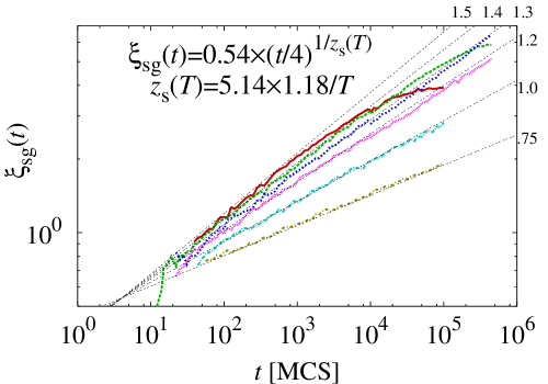
Figure 4: (Color online) Relaxation functions of the spin-glass correlation length in the Ising model. The temperatures are denoted aside the fitting lines.

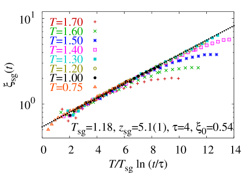
Figure 5: (Color online) The spin-glass correlation length in the Ising model is plotted against $T/T_{\mathrm{sg}}\ln(t/\tau)$ using $\tau=4$ and $T_{\mathrm{sg}}=1.18$. A fitting line with $z_{\mathrm{sg}}=5.1$ is plotted by dotted line.

IV.2 Finite-time-scaling analysis of $\chi_{\mathrm{sg}}$

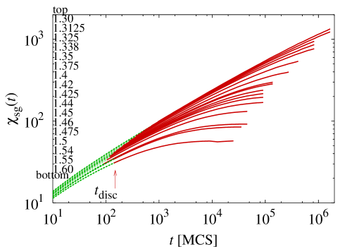
Figure 6: (Color online) Relaxation functions of the spin-glass susceptibility in the Ising model. Relaxation data after $t_{\mathrm{disc}}$ (red curves) are used in the scaling analysis.

The relaxation functions of the spin-glass susceptibility $\chi_{\mathrm{sg}}(t)$ are plotted in Fig. 6. We perform the finite-time scaling analysis using these data. We discard data in the initial relaxation regime before the $t_{\mathrm{disc}}$ step, which are depicted in Fig. 6. A typical value for $t_{\mathrm{disc}}$ varies between 100 and 1000. The initial relaxation is very short compared to the equilibrium relaxation.

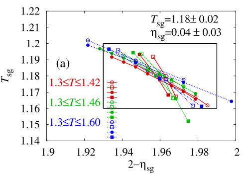
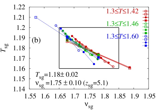
Figure 7: (Color online) Estimates of the finite-time-scaling parameters in the Ising model. (a) $T_{\mathrm{sg}}$ versus $2-\eta_{\mathrm{sg}}$. (b) $T_{\mathrm{sg}}$ versus $\nu_{\mathrm{sg}}$. For each temperature range, we plot results of two different procedures (circle and square symbols) and two different discarding steps (filled and unfilled symbols). Rectangles depict error ranges, which covers most of possible scaling parameter sets.

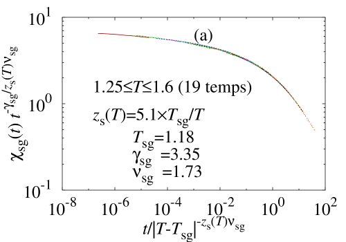
Figure 8: (Color online) Finite-time-scaling plots in the Ising model. (a) A scaling plot of $\chi_{\mathrm{sg}}$ using the obtained results. (b) A scaling plot of the correlation length in the equilibrium convergence.

We follow the procedures explained in Sec. III.2. Three different temperature ranges are considered in this analysis. One consists of all the 17 temperatures of Fig. 6 ranging $1.3\leq T\leq 1.6$. The second one consists of the lower 12 temperatures ranging $1.3\leq T\leq 1.46$. The third one consists of the lower 8 temperatures ranging $1.3\leq T\leq 1.42$. For each temperature range, we adopt three procedures of estimating the scaling parameters. We find that the procedure-2 and the procedure-3 yield consistent results. Therefore, we compare results of procedure-1 and procedure-2. We also change the discarding time step, which is distinguished in Fig. 7 with filled and unfilled symbols. Unfilled symbols depict data when the first $t_{\mathrm{disc}}$ steps are discarded, where $t_{\mathrm{disc}}$ are as depicted in Fig. 6. Filled symbols depict data of discarding the first $3t_{\mathrm{disc}}$ steps.

Figure 7(a) shows the obtained critical temperature plotted versus $2-\eta_{\mathrm{sg}}$. Behaviors of the estimated critical temperature depends on the procedures, the temperature ranges, and the discarding steps. These data seem to cross or merge at the most probable parameter point of $(2-\eta_{\mathrm{sg}},T_{\mathrm{sg}})\simeq(1.96,1.18)$. We put error bars so that they cover most of possible scaling parameters. Figure 7(b) shows the critical temperature plotted versus the critical exponent $\nu_{\mathrm{sg}}$. The scaling results cross or merge at $(\nu_{\mathrm{sg}},T_{\mathrm{sg}})\simeq(1.73,1.18)$. Two estimates for the transition temperature are consistent. An exponent $\gamma_{\mathrm{sg}}$ is estimated from $\eta_{\mathrm{sg}}$ and $\nu_{\mathrm{sg}}$. Using the estimated scaling parameters we plot the scaling functions in Fig. 8(a). We also plot in Fig. 8(b) a result of the finite-time scaling analysis of the dynamic correlation length. It yields the following scaling relation:

$$\xi_{\mathrm{sg}}(t)t^{-1/z_{\mathrm{s}}(T)}=\tilde{\xi}_{\mathrm{sg}}(t/(T-T_{\mathrm{sg}})^{-z_{\mathrm{s}}(T)\nu_{\mathrm{sg}}})$$ (18)

The shape of the universal scaling function is robust against changes of discarding steps and the temperature ranges.

From the present scaling analysis, we conclude the critical temperature and the critical exponents of the Ising model in three dimensions:

$$T_{\mathrm{sg}} = 1.18\pm 0.02$$ (19)

$$\gamma_{\mathrm{sg}} = 3.4\pm 0.2$$ (20)

$$\nu_{\mathrm{sg}} = 1.75\pm 0.10$$ (21)

$$\eta_{\mathrm{sg}} = 0.04\pm 0.03$$ (22)

$$z_{\mathrm{sg}} = 5.1\pm 0.1.$$ (23)

Previous estimates Bhatt ; Ogielski ; KawashimaY ; palassini ; ballesteros ; maricampbell for $T_{\mathrm{sg}}$ lie between 1.1 and 1.2. They are roughly categorized into two groups. Group I: $T_{\mathrm{sg}}$ close to 1.1 and $\nu_{\mathrm{sg}}$ close to 2.KawashimaY ; ballesteros Group II: $T_{\mathrm{sg}}$ close to 1.2 and $\nu_{\mathrm{sg}}$ close to 1.3.Bhatt ; Ogielski ; maricampbell Our estimate for $T_{\mathrm{sg}}$ belongs to the latter group. On the other hand, an estimate for $\nu_{\mathrm{sg}}$ is rather close to the former group and agrees with the experimental result,Aruga which is $\nu_{\mathrm{sg}}\sim 1.7$. It is very hard to determine a value of $\nu_{\mathrm{sg}}$.

Recently, Campbell et. al. campbell-huku-taka claimed that a choice of a scaling variable may affect the scaling results. Particularly, a value of $\nu$ changes. We applied their method and checked the claim. A scaling plot is possible with $T_{\mathrm{sg}}=1.18$, $\nu_{\mathrm{sg}}=2.18$, and $\gamma_{\mathrm{sg}}=4.15$, when we use a scaling vaiable $(\beta_{\mathrm{sg}}-\beta)$ instead of $(T-T_{\mathrm{sg}})$. The critical temperature and the anomalous exponenet $\eta_{\mathrm{sg}}$ are not affected by this change. We consider that these two estimates are reliable. To the contrary, two exponents, $\nu_{\mathrm{sg}}$ and $\gamma_{\mathrm{sg}}$, become larger than our original estimates and are consistent with the values of group I. We cannot exclude out either estimate within our amount of simulations.

V Results of the XY model

V.1 Brief introduction to the vector models

It is widely accepted that the spin-glass transition occurs in the Ising model.Bhatt ; Ogielski ; KawashimaY ; palassini ; ballesteros ; maricampbell However, spins of many spin-glass materials are of the Heisenberg type. Early numerical investigations McMillan ; Morris ; Olive concluded that there is no spin-glass transition in this model. Kawamura KawamuraXY1 ; KawamuraXY2 ; KawamuraXY3 ; KawamuraH1 proposed the chirality-mechanism in order to explain the real spin-glass transition. The spin-glass transitions in real materials occur driven by the chiral-glass transition. This scenario assumes that there is no spin-glass transition in the isotropic model.HukushimaH ; HukushimaH2 Recently, there are several investigations which suggest the simultaneous transition.Matsubara3 ; Matsubara4 ; Endoh2 ; nakamura ; Lee

The situation is same in the XY spin-glass model in three dimensions. A domain-wall energy analysis Morris and a Monte Carlo simulation analysis Jain found no spin-glass transition. However, a possibility of a finite spin-glass transition has been suggested by recent investigations Lee ; Maucourt ; Kosterlitz ; Granato ; yamamoto1 . Since the chirality is defined by spin variables, the chiral-glass transition occurs trivially if the spin-glass transition occurs. Therefore, it is crucial to check whether or not both transitions occur at the same temperature. This is a very naive problem. For example, the spin-chirality separation is observed in the fully frustrated nonrandom XY model in two dimensions.OzIto2 However, the difference between the critical temperatures is only 1%.

V.2 Dynamic correlation length

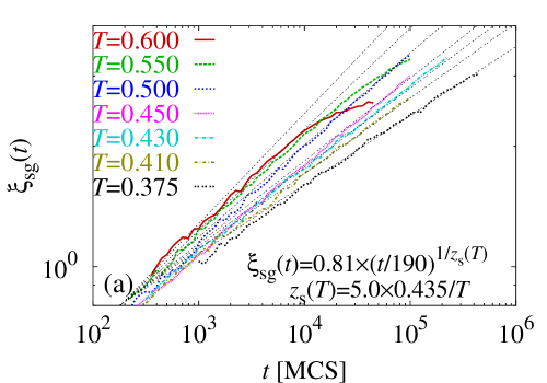
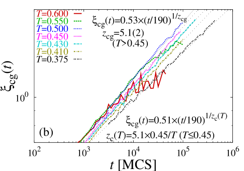
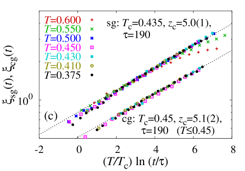
Figure 9: (Color online) Relaxation functions of the correlation lengths in the XY model. (a) The spin-glass correlation length. (b) The chiral-glass correlation length. (c) Scaling plots of $\xi_{\mathrm{sg}}$ and $\xi_{\mathrm{cg}}$ versus $T/T_{\mathrm{c}}\ln(t/\tau)$. Scaling parameters are as denoted in the figure. The chiral-glass scaling is only possible at $T\leq 0.45$.

Relaxation functions of the spin- and the chiral-glass correlation length are shown in Figs. 9(a) and (b). Algebraic behaviors are observed in the nonequilibrium relaxation process both above and below the critical temperature. Slope of relaxation functions of the spin-glass correlation length continuously depends on the temperature. There is no anomaly at the transition temperature, $T_{\mathrm{sg}}=0.435$, which will be estimated in the next subsection. This is the same behavior with the Ising model. On the other hand, relaxation functions of the chiral-glass correlation length do not depend on the temperature at higher temperatures ($T\geq 0.45$). It changes the behavior at $T\simeq 0.45$ becoming temperature-dependent at lower temperatures. This is a distinct difference between the spin- and the chiral-glass nonequilibrium dynamics. From the scaling analysis of the correlation lengths, we obtain the temperature dependences of the nonequilibrium dynamic exponents. Figure 9(c) shows results of the scaling. The scaling is possible both below and above $T_{\mathrm{sg}}$ for the spin-glass correlation length, but it is only possible below $T_{\mathrm{sg}}\simeq T_{\mathrm{cg}}=0.45$ for the chiral-glass one. It is also noted that a characteristic time is common between the spin and the chirality, and it is larger than the Ising one.

We obtain temperature dependences of the dynamic exponent for the spin glass ($z_{\mathrm{s}}(T)$) and the chiral glass ($z_{\mathrm{c}}(T)$) as follow.

$$z_{\mathrm{s}}(T) = (5.0\pm 0.1)\times\frac{0.435}{T}$$ (24)

$$z_{\mathrm{c}}(T) = (5.1\pm 0.2)~{}~{}~{}~{}~{}~{}~{}~{}~{}~{}~{}~{}~{}(T>0.45)$$ (25)

$$z_{\mathrm{c}}(T) = (5.1\pm 0.2)\times\frac{0.45}{T}~{}~{}~{}(T\leq 0.45)$$ (26)

Here, we use $T_{\mathrm{sg}}=0.435$ and $T_{\mathrm{cg}}=0.45$, which will be estimated in the next subsection. A coefficient to the temperature-ratio term is the dynamic critical exponent at the transition temperature. It agrees with each other within error bars. Therefore, the dynamic critical exponents of the spin-glass and the chiral-glass transitions are considered to take the same value. The nonequilibrium dynamic exponent of the chiral glass changes behavior when the spin-glass exponent equals to the the chiral-glass one. The spin-glass transition occurs at this temperature. Both exponents behave in the same manner below the temperature.

V.3 Finite-time-scaling analysis of $\chi_{\mathrm{sg}}$ and $\chi_{\mathrm{cg}}$

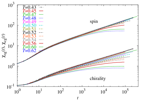
Figure 10: (Color online) Relaxation functions of the spin- and the chiral-glass susceptibility in the XY model.

Figure 10 shows the relaxation functions of the spin- and the chiral-glass susceptibility. Some of the data are taken from our previous work.yamamoto1 We added several temperature points and increased a total Monte Carlo step particularly near the transition temperature. In the previous work, we supposed that the dynamic exponent is independent from the temperature. Crossing behaviors of the scaling results were not good. Consequently, the error bars of obtained results became large. These failures are possibly due to the temperature dependence of the nonequilibrium dynamic exponent. In the present analysis we use Eqs. (24) and (25). A scaling procedure is same as the Ising case.

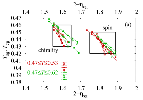
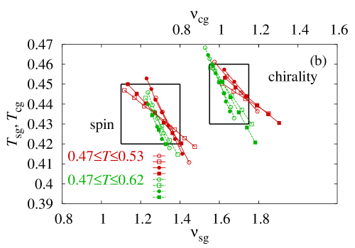
Figure 11: (Color online) Estimations of the finite-time-scaling parameters in the XY model. (a) $T_{\mathrm{c}}$ versus $2-\eta$. (b) $T_{\mathrm{c}}$ versus $\nu$. Spin-glass(chiral-glass) results are plotted against the lower(upper) x-axis. The circle symbols are results of the scaling procedure-1, and the square symbols are those of the procedure-2. Unfilled symbols depict data when the first 400 steps are discarded. Filled symbols depict data when the first 1000 steps are discarded.

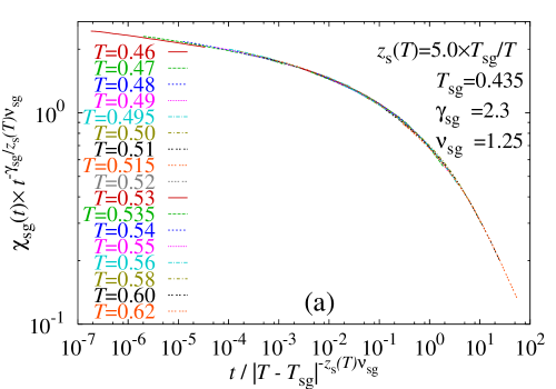
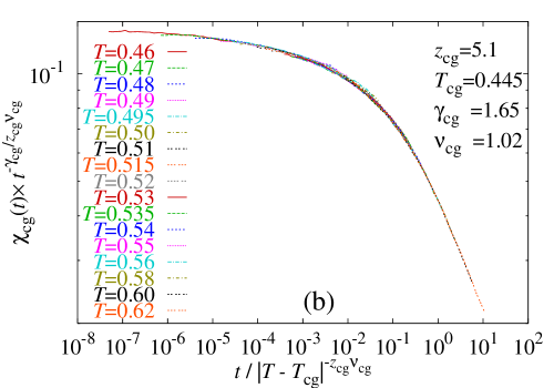
Figure 12: (Color online) Finite-time-scaling plots of (a) $\chi_{\mathrm{sg}}$ and (b) $\chi_{\mathrm{cg}}$ using the estimated scaling parameters in the XY model.

Figures 11 (a) and (b) show estimations of the scaling parameters. We determine the best estimates from the figure so that the results are robust against the difference of procedures. For the spin-glass transition:

$$T_{\mathrm{sg}} = 0.435\pm 0.015$$ (27)

$$\gamma_{\mathrm{sg}} = 2.30\pm 0.25$$ (28)

$$\nu_{\mathrm{sg}} = 1.25\pm 0.15$$ (29)

$$\eta_{\mathrm{sg}} = 0.18\pm 0.07$$ (30)

$$z_{\mathrm{sg}} = 5.0\pm 0.1.$$ (31)

For the chiral-glass transition:

$$T_{\mathrm{cg}} = 0.445\pm 0.015$$ (32)

$$\gamma_{\mathrm{cg}} = 1.65\pm 0.20$$ (33)

$$\nu_{\mathrm{cg}} = 1.05\pm 0.10$$ (34)

$$\eta_{\mathrm{cg}} = 0.40\pm 0.05$$ (35)

$$z_{\mathrm{cg}} = 5.1\pm 0.2.$$ (36)

The spin- and the chiral-glass transition temperatures cannot be distinguished to be different. The chiral-glass transition occurs at a little higher temperature but the difference is within the error bars. A value of the dynamic critical exponent coincides with each other within the error bar. Both transitions are considered to be dynamically universal. On the other hand, the static exponents take different values.

The scaling plot using the obtained results is shown in Figs. 12(a) and (b). All data suitably fall onto a single scaling function. The obtained transition temperature is between our previous estimate yamamoto1 supposing a constant dynamic exponent and other estimates.KawamuraXY3 ; Granato Our previous estimates are $T_{\mathrm{sg}}=0.455(15)$, $\gamma_{\mathrm{sg}}=1.7(2)$, $z_{\mathrm{sg}}\nu_{\mathrm{sg}}=4.8(4)$ for the spin-glass transition and $T_{\mathrm{cg}}=0.467(10)$, $\gamma_{\mathrm{cg}}=1.4(1)$, and $z_{\mathrm{cg}}\nu_{\mathrm{cg}}=4.7(2)$ for the chiral-glass transition. The results of the spin-glass transition are strongly influenced by the temperature dependence of $z_{\mathrm{s}}(T)$. Granato Granato provided the following for the spin-glass transition: $T_{\mathrm{sg}}=0.39(2)$, $\nu=1.2(2)$, and $z=4.4(3)$. Kawamura and Li KawamuraXY3 provided the following for the chiral-glass transition: $T_{\mathrm{cg}}=0.39(3)$, $\nu=1.2(2)$, $\gamma/\nu=1.85(20)$, and $z=7.4(10)$. These transition temperatures are lower then our present estimates.

VI Results of the Heisenberg model

VI.1 Dynamic correlation length

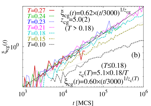
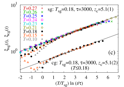
Figure 13: (Color online) Relaxation functions of the correlation lengths in the Heisenberg model. (a) The spin-glass correlation length. (b) The chiral-glass correlation length. Fitting lines are plotted with broken lines. (c) The scaling plot of $\xi_{\mathrm{sg}}$ plotted versus $T/T_{\mathrm{sg}}\ln(t/\tau)$.

Relaxation functions of the spin- and the chiral-glass correlation lengths are shown in Figs. 13(a) and (b). We observe algebraic increases of both correlation lengths. We estimate the dynamic exponent using these data.

The chiral-glass exponent may have a rather large error bar because numerical fluctuations of the chiral-glass data are large. Evaluatios of the chiral-glass quantities are generally difficult because the chiral-glass correlations are much smaller than the spin-glass ones as shown in Fig. 1(b). It is necessary to increase a sample number in order to suppress the fluctuations. Within the present computational facilities, it is not realistic to increase a Monte Carlo step number until the chiral-glass correlation length grows comparable to the present spin-glass data. For example, we need a hundred times longer steps to wait until $\xi_{\mathrm{cg}}$ reaches five lattice spacings.

It is also noted that the algebraic increase in the low-temperature phase appears later as the temperature decrease. It is considered to be an outcome of the slow dynamics of the spin-glass phase. A time range to estimate the dynamic exponent is restricted to be short. Reliability of the estimated value may become poor.

Even though the numerical fluctuations are large, we observe a temperature-dependence of the dynamic exponent as in the Ising model and the XY model. Logarithmic slope of the spin-glass correlation length depends on the temperature irrespective of the transition temperature. That of the chiral-glass correlation length depends on the temperature only when $T<0.18$. These evidences are checked by a scaling plot of Fig. 13(c). The spin-glass data can be scaled to a single line both above and below the critical temperature, $T_{\mathrm{sg}}=0.18$, which will be estimated in the next subsection. On the other hand, the chiral-glass data are scaled only below $T_{\mathrm{sg}}$. The high temperature data systematically deviate from the scaling line. They are better approximated by a temperature-independent algebraic function: $\xi_{\mathrm{cg}}=0.62\times(t/3000)^{1/5.0}$. Therefore, the chiral-glass dynamic exponent is constant above $T_{\mathrm{sg}}$ and becomes temperature dependent below $T_{\mathrm{sg}}$. The temperature dependence of the chiral-glass dynamic exponent below $T_{\mathrm{sg}}$ is same as the spin-glass one. These behaviors are same as the XY model. A difference is a characteristic time $\tau$, which is much larger than the Ising and the XY models.

The temperature dependences of the nonequilibrium dynamic exponent in the Heisenberg model, $z_{\mathrm{s}}(T)$ for the spin glass $z_{\mathrm{c}}(T)$ for the chiral glass, are summarized as follow.

$$z_{\mathrm{s}}(T) = (5.1\pm 0.1)\times\frac{0.18}{T}$$ (37)

$$z_{\mathrm{c}}(T) = (5.0\pm 0.2)~{}~{}~{}~{}~{}~{}~{}~{}~{}~{}~{}~{}~{}(T>0.18)$$ (38)

$$z_{\mathrm{c}}(T) = (5.1\pm 0.2)\times\frac{0.18}{T}~{}~{}~{}(T\leq 0.18)$$ (39)

Values of the nonequilibrium dynamic exponent at $T=T_{\mathrm{sg}}=0.18$ agree with each other. This is the temperature where the chiral-glass dynamic exponent changes the behavior. It can be considered that dominant dynamics changes when the $T$-dependent $z_{\mathrm{s}}(T)$ catches up with the $T$-independent $z_{\mathrm{c}}(T)$ at $T=0.18$. The spin-glass nonequilibrium dynamic exponent, $z_{\mathrm{s}}(T)$, is larger than the chiral-glass dynamic critical exponent, $z_{\mathrm{cg}}$, below the temperature. Then, the dynamics of the chirality obeys that of the spin because the chirality is defined by the spin. As the result, $z_{\mathrm{c}}(T)$ behaves in a same manner with $z_{\mathrm{s}}(T)$.

VI.2 Finite-time-scaling analysis of $\chi_{\mathrm{sg}}$ and $\chi_{\mathrm{cg}}$

Figure 14: (Color online) Relaxation functions of the spin-glass and the chiral-glass susceptibility in the Heisenberg model. Data of the chiral-glass susceptibility are multiplied by 535 in order to show in the same scale with the spin-glass susceptibility.

Figure 14 shows relaxation functions of the spin- and the chiral-glass susceptibility. Data of the chiral-glass susceptibility are multiplied by 535 in order to show them in a same scale with the spin-glass susceptibility. Amplitude of the chiral-glass susceptibility is roughly 1000 times smaller than the spin-glass one. The chiral-glass order is very small.

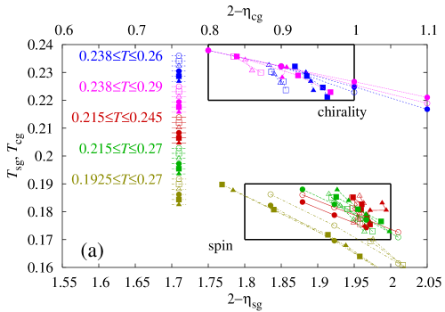
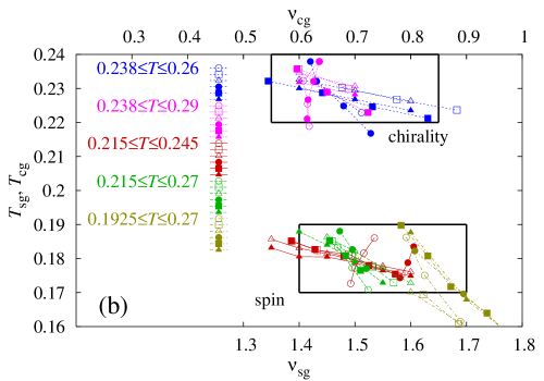
Figure 15: (Color online) Estimations of finite-time-scaling parameters in the Heisenberg model. (a) $T_{\mathrm{sg/cg}}$ versus $2-\eta_{\mathrm{sg/cg}}$. (b) $T_{\mathrm{sg/cg}}$ versus $\nu_{\mathrm{sg/cg}}$. Spin-glass(chiral-glass) results are plotted against the lower(upper) axis. The circle symbols are results of the scaling procedure-1, the squares are of the procedure-2, and the triangles are of the procedure-3. Unfilled symbols depict data of 1000 discarding steps, and filled symbols depict those of 3000 steps. Color distinguishes the temperature range of data used in the scaling analysis. Results of $0.1925\leq T\leq 0.27$ are obtained by discarding 3000 steps (unfilled symbols) and 10000 steps (filled symbols).

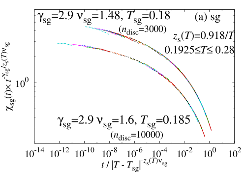
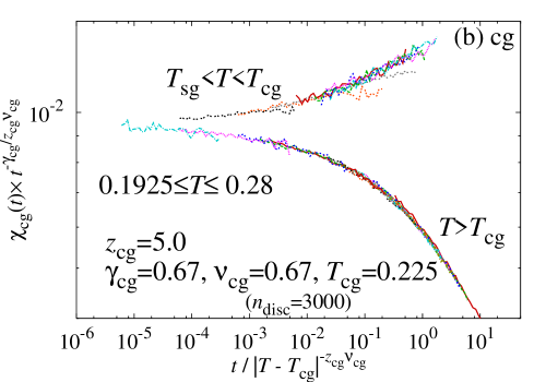
Figure 16: (Color online) (a)A finite-time-scaling plots of $\chi_{\mathrm{sg}}$ using the estimated parameters. Two possible chioces of scaling parameters are shown. As we discard more steps, a value of $\nu_{\mathrm{sg}}$ increases. (b) A scaling plot of $\chi_{\mathrm{cg}}$. Data of the chiral-glass phase, $T_{\mathrm{sg}}<T<T_{\mathrm{cg}}$, are also scaled using the same parameters.

Figures 15 (a) and (b) show estimations of scaling parameters. We obtain the transition temperature and the critical exponents, where the scaling results are robust against the change of procedures. It is clear from the figures that the spin-glass transition and the chiral-glass transition occur at different temperatures. Error bars of the critical exponents are rather large compared to those of transition temperatures. Particularly, a value of $\nu_{\mathrm{sg}}$ systematically shifts to a higher side when we decrease the lowest temperature of data used in the scaling analysis from $T=0.215$ to $T=0.1925$. Then, a value of $\eta_{\mathrm{sg}}$ is influenced. However, a value of $\gamma_{\mathrm{sg}}$ does not change. Our estimates for the spin-glass transition are

$$T_{\mathrm{sg}} = 0.18\pm 0.01$$ (40)

$$\gamma_{\mathrm{sg}} = 2.9\pm 0.2$$ (41)

$$\nu_{\mathrm{sg}} = 1.55\pm 0.15$$ (42)

$$\eta_{\mathrm{sg}} = 0.1\pm 0.1$$ (43)

$$z_{\mathrm{sg}} = 5.1\pm 0.1,$$ (44)

and those for the chiral-glass transition are

$$T_{\mathrm{cg}} = 0.23\pm 0.01$$ (45)

$$\gamma_{\mathrm{cg}} = 0.65\pm 0.15$$ (46)

$$\nu_{\mathrm{cg}} = 0.70\pm 0.15$$ (47)

$$\eta_{\mathrm{cg}} = 1.1\pm 0.1$$ (48)

$$z_{\mathrm{cg}} = 5.0\pm 0.2.$$ (49)

In our previous work,nakamura we assumed that the dynamic exponent does not depend on the temperature. The obtained results are $T_{\mathrm{sg}}=0.21^{+0.01}_{-0.03}$ and $T_{\mathrm{cg}}=0.22^{+0.01}_{-0.04}$. Present estimates roughly correspond to the upper and the lower bound of the previous estimates. The error bars shrink, and two transitions are resolved to be different, which is made possible taking into acount the temperature dependence of the spin-glass dynamic exponent. Therefore, the spin-glass results are much influenced. Results of the chiral-glass transition are consistent with the previous ones, because an assumption of a constant dynamic exponent is good in this case. Even though the static exponent, $\nu_{\mathrm{sg}}$ and $\gamma_{\mathrm{sg}}$, take different values, $z_{\mathrm{sg}}$ and $z_{\mathrm{cg}}$ coincide within the error bars. They also agree with the dynamic critical exponents of the Ising and the XY models. The spin-glass and the chiral-glass transitions in three dimensions can be considered to be dynamically universal.

Scaling plots using the obtained results are shown in Figs. 16(a) and (b). For the spin-glass transition, we plot two results with different choices of scaling parameters. They are within the error bars of our estimates. A value of $\nu_{\mathrm{sg}}$ tends to increase when the lowest temperature of the scaling data decreases and when we increase the discarding steps. The transition temperature and a value of $\gamma_{\mathrm{sg}}$ are rather robust against these changes. A scaling plot using a parameter set with $\nu_{\mathrm{sg}}=1.48$ shows some systematic deviations in the long time limit at low temperatures. Therefore, our best choice in the present analysis is $\gamma_{\mathrm{sg}}=2.9$, $\nu_{\mathrm{sg}}=1.6$, and $T_{\mathrm{sg}}=0.185$. A ratio of scaling parameter, $\gamma_{\mathrm{sg}}/\nu_{\mathrm{sg}}$, agrees with the logarithmic slope of the spin-glass susceptibility of Fig. 14 at $T=T_{\mathrm{sg}}$.

For the chiral-glass transition, we plot data both above and below the chiral-glass transition temperature. A scaling to a single curve is good above the chiral-glass transition temperature. A scaling is also possible for the data in the chiral-glass phase: $T_{\mathrm{sg}}<T<T_{\mathrm{cg}}$. The scaling function is bending upward, which suggests that a ratio of critical exponent, $\gamma/\nu$, is increasing as the temperature decreases.

We also applied the $\beta$-scaling proposed by Campbell et. al.campbell-huku-taka and checked our estimates. As in the Ising model, the critical temperature and the anomalous exponent $\eta_{\mathrm{sg}}$ do not change, while $\nu_{\mathrm{sg}}$ and $\gamma_{\mathrm{sg}}$ increase. The estimates are $T_{\mathrm{sg}}=0.18$, $\nu_{\mathrm{sg}}=3.7$, and $\gamma_{\mathrm{sg}}=6.4$. Two exponents, $\nu_{\mathrm{sg}}$ and $\gamma_{\mathrm{sg}}$, become particlarly large. The present numerical data may be insufficient to determine these critical exponents. On the other hand, the spin-glass transition temperature is consistent with our original estimate. We obtained this value by two scaling analyses and by a temperature dependence of the chiral-glass dynamic exponent. We consider that the value is very reliable.

VII Summary and Discussion

The nonequilibrium dynamics and the spin-glass transitions in three dimensions are clarified in detail. It is confirmed that the nonequilibrium dynamic exponent of the spin glasses continuously depends on the temperature without anomaly at the transition temperature. The spin-glass dynamics in the high-temperature phase smoothly continues to the low-temperature phase. The frozen-spin domain grows in the algebraic law controlled by $z_{\mathrm{s}}(T)$ irrespective of the critical temperature. The growth in the high-temperature phase stops when the domain size reaches the equilibrium value. The smooth temperature dependence of the nonequilibrium dynamic exponent is considered to be a common characteristic behavior of the spin glasses. We will need to explain the origin regardless the spin-glass transition, which is left for the future study.

In the vector spin models, the nonequilibrium dynamic exponent of the chiral glass shows a different behavior. It does not depend on the temperature above the “spin-glass transition temperature”. It remains constant until it changes the behavior at $T=T_{\mathrm{sg}}$. When $T<T_{\mathrm{sg}}$, the chiral-glass dynamic exponent is same with the spin-glass one. Therefore, the dynamics of the chiral glass is essentially same with the spin-glass dynamics in the low-temperature phase. They are different only in the high-temperature phase.

Our observation suggests the following scenario. Dynamics of the spin and the chirality are separated at temperatures above $T_{\mathrm{sg}}$. The dynamic exponent of the spin glass is smaller than the chiral-glass one. The spin-glass state evolves with time faster than the chiral-glass state. Therefore, the chiral glass freezes first at a higher temperature. This is the chiral-glass transition as KawamuraKawamuraXY1 ; KawamuraXY2 ; KawamuraXY3 ; KawamuraH1 proposed. Since the spin and the chirality are separated, the spin-glass dynamic exponent shows no anomaly at $T=T_{\mathrm{cg}}$. The situation changes at $T=T_{\mathrm{sg}}$, where the spin-glass dynamic exponent overcomes the chiral-glass dynamic critical exponent, $z_{\mathrm{cg}}$. The spin-glass transition occurs at this temperature. The value, $z_{\mathrm{sg}}=z_{\mathrm{cg}}\simeq 5.1$, is found to be common to all the spin-glass models in three dimensions. Below the spin-glass transition temperature, the spin-glass dynamics is slower than the chiral-glass dynamics above $T_{\mathrm{sg}}$, because $z_{\mathrm{s}}(T)>z_{\mathrm{cg}}$. Since the chirality is defined by the spin variables, the chirality obeys the spin dynamics once the spin freezes and the spin-glass dynamics becomes dominant. The spin and the chirality is coupled below $T_{\mathrm{sg}}$, and both dynamic exponents show the same temperature dependence. Therefore, this is the spin-glass phase.

Using the obtained temperature dependences of the dynamic exponent we performed the finite-time-scaling analysis on the spin- and the chiral-glass susceptibility. The transition temperature and the critical exponents are estimated with high precisions. In the Ising model, the results are compared with the previous works Bhatt ; Ogielski ; KawashimaY ; palassini ; ballesteros ; maricampbell and the experimental result.Aruga We also checked that a change of a scaling variable may affect a value of $\nu_{\mathrm{sg}}$. In the XY model, the spin- and the chiral-glass transitions occur at the almost same temperature. In the Heisenberg model, the spin- and the chiral-glass transitions are resolve to be different. It is the lower and the upper bound of our previous estimate.nakamura Therefore, it becomes clear that the chiral-glass transition without the spin-glass order occurs in the Heisenberg model, as the chirality-mechanism predicted. KawamuraXY1 ; KawamuraXY2 ; KawamuraXY3 ; KawamuraH1 ; HukushimaH ; HukushimaH2 The chiral-glass phase continues for $T_{\mathrm{cg}}\geq T\geq T_{\mathrm{sg}}$.

The chirality mechanism insists that the spin-chirality separation is only observed in the long time and in the large size limit.HukushimaH2 A crossover from the spin-chirality coupling regime at short scales to the decoupling regime at long scales is considered to be important. Discrepancy regarding whether the simultaneous spin-chirality transition occurs or not is explained by the crossover. It is considered that the true transition will not be observed unless the simulation goes beyond the crossover length-time scale. However, we are able to observe the spin-chirality separation near the chiral-glass transition temperature within a rather short time and a small length scale. It was made possible by clarifying the temperature dependence of the dynamic exponent in the nonequilibrium relaxation process. The separation is observed as a different temperature dependence. If we neglect the effect of the temperature dependence, the spin-chirality separation will be smeared out. Then, we are lead to the simultaneous transition.

All the dynamic critical exponents at the transition temperatures investigated in this paper take almost the same value. It may be the universal exponent controlling the spin-glass transitions. Therefore, we consider the dynamical universality about the spin- and the chiral-glass transitions in three dimensions.

The spin-glass dynamics around the transition temperature has exotic behaviors, which are quite different from the regular systems. A single continuous phase seems to exist in regard with the dynamics. It should be explained in connection with the picture of the low-temperature phase. It will be a future subject.

- (1) K. Binder and A. P. Young, Rev. Mod. Phys. 58, 801 (1986).
- (2) J. A. Mydosh, Spin Glasses (Taylor & Francis, London, 1993).
- (3) Spin Glasses and Random Fields edited by A. P. Young (World Scientific, Singapore, 1997).
- (4) V. Dupuis, E. Vincent, J.-P. Bouchaud, J. Hammann, A. Ito, and H. A. Katori, Phys. Rev. B 64, 174204 (2001).
- (5) P. E. Jönsson, H. Yoshino, P. Nordblad, H. Aruga Katori, and A. Ito, Phys. Rev. Lett. 88, 257204 (2002).
- (6) J.-P. Bouchaud, F. Krzakala, and O. C. Martin, Phys. Rev. B 68, 224404 (2003).
- (7) F. Bert, V. Dupuis, E. Vincent, J. Hammann, and J.-P. Bouchaud, Phys. Rev. Lett. 92, 167203 (2004).
- (8) D. S. Fisher and D. A. Huse, Phys. Rev. Lett. 56, 1601 (1986); Phys. Rev. B 38, 373 (1988); 38, 386 (1988).
- (9) J.-P. Bouchaud, V. Dupuis, J. Hammann, and E. Vincent, Phys. Rev. B 65, 024439 (2001).
- (10) H. Yoshino, A. Lemaître, and J.-P. Bouchaud, Eur. Phys. J. B 20, 367 (2001).
- (11) L. Berthier and P. C. W. Holdsworth, Europhys. Lett. 58, 35 (2002).
- (12) F. Scheffler, H. Yoshino, and P. Maass, Phys. Rev. B 68, 060404(R) (2003).
- (13) H. Yoshino, J. Phys. A 36 10 819 (2003).
- (14) G. Parisi, F. Ricci-Tersenghi, and J. J. Ruiz-Lorenzo, J. Phys. A 29, 7943 (1996).
- (15) J. Kisker, L. Santen, M. Schreckenberg, and H. Rieger, Phys. Rev. B 53, 6418 (1996).
- (16) T. Komori, H. Yoshino, and H. Takayama, J. Phys. Soc. Jpn. 68, 3387 (1999); 69, 228 (2000); 69, 1192 (2000).
- (17) L. Berthier and J.-P. Bouchaud, Phys. Rev. B 66 054404 (2002); Phys. Rev. Lett. 90, 059701 (2003).
- (18) H. Yoshino, K. Hukushima, and H. Takayama, Phys. Rev. B 66, 064431 (2002).
- (19) T. Nakamura and T. Yamamoto, Prog. Theor. Phys. Suppl. 157, 42 (2005).
- (20) V. Dupuis, E. Vincent, J.-P. Bouchaud, J. Hammann, A. Ito, and H. A. Katori, Phys. Rev. B 64, 174204 (2001).
- (21) P. E. Jönsson, H. Yoshino, and P. Nordblad, Phys. Rev. Lett. 89, 097201 (2002).
- (22) L. Berthier and A. P. Young, Phys. Rev. B 69, 184423 (2004).
- (23) H. G. Katzgraber and I. A. Campbell, Phys. Rev. B 72 014462 (2005).
- (24) D. A. Huse, Phys. Rev. B 40, 304 (1989).
- (25) R. E. Blundell, K. Humayun, and A. J. Bray, J. Phys. A: Math. Gen. 25, L733 (1992).
- (26) D. Stauffer, Physica A 186, 197 (1992).
- (27) N. Ito, Physica A, 192, 604 (1993).
- (28) N. Ito and Y. Ozeki, Int. J. Mod. Phys. 10, 1495 (1999).
- (29) Y. Ozeki and N. Ito Phys. Rev. B 68, 054414 (2003).
- (30) T. Shirahata and T. Nakamura, Phys. Rev. B 65, 024402 (2001).
- (31) T. Nakamura and S. Endoh, J. Phys. Soc. Jpn. 71, 2113 (2002).
- (32) T. Nakamura, S. Endoh, and T. Yamamoto, J. Phys. A 36, 10895 (2003).
- (33) T. Shirahata and T. Nakamura, J. Phys. Soc. Jpn. 73, 254 (2004).
- (34) T. Yamamoto, T. Sugashima, and T. Nakamura, Phys. Rev. B 70, 184417 (2004).
- (35) T. Nakamura, Phys. Rev. B 71, 144401 (2005).
- (36) H. Kawamura and M. Tanemura, J. Phys. Soc. Jpn. 60, 608 (1991).
- (37) H. Kawamura, Phys. Rev. B 51, 12398 (1995).
- (38) H. Kawamura and M. S. Li, Phys. Rev. Lett. 87, 187204 (2001).
- (39) H. Kawamura, Phys. Rev. Lett. 68, 3785 (1992).
- (40) K. Hukushima and H. Kawamura, Phys. Rev. E 61, R1008 (2000).
- (41) K. Hukushima and H. Kawamura, Phys. Rev. B 72, 144416 (2005).
- (42) J. A. Olive, A. P. Young, and D. Sherrington, Phys. Rev. B 34, 6341 (1986).
- (43) R. N. Bhatt and A. P. Young, Phys. Rev. Lett. 54, 924 (1985).
- (44) A. T. Ogielski and I. Morgenstern, Phys. Rev. Lett. 54, 928 (1985).
- (45) N. Kawashima and A. P. Young, Phys. Rev. B 53, R484 (1996).
- (46) M. Palassini and S. Caracciolo, Phys. Rev. Lett. 82 5128 (1999).
- (47) H. G. Ballesteros, A. Cruz, L. A. Fernández, V. Martin-Mayor, J. Pech, J. J. Ruiz-Lorenzo, A. Tarancón, P. Téllez, C. L. Ullod, and C. Ungil, Phys. Rev. B 62, 14 237 (2000).
- (48) P. O. Mari and I. A. Campbell, Phys. Rev. B 65, 184409 (2002).
- (49) K. Gunnarsson, P. Svedlindh, P. Nordblad, L. Lundgren, H. Aruga and A. Ito, Phys. Rev. B 43, 8199 (1991).
- (50) I. A. Campbell, K. Hukushima, and H. Takayama, cond-mat/0603453.
- (51) W. L. McMillan, Phys. Rev. B 31, 342 (1985).
- (52) B. W. Morris, S. G. Colborne, M. A. Moore, A. J. Bray, and J. Canisius, J. Phys. C 19, 1157 (1986).
- (53) F. Matsubara, S. Endoh, and T. Shirakura, J. Phys. Soc. Jpn. 69, 1927 (2000).
- (54) F. Matsubara, T. Shirakura, and S. Endoh, Phys. Rev. B 64, 092412 (2001).
- (55) S. Endoh, F. Matsubara, and T. Shirakura, J. Phys. Soc. Jpn 70, 1543 (2001).
- (56) L. W. Lee and A. P. Young, Phys. Rev. Lett. 90, 227203 (2003).
- (57) S. Jain and A. P. Young, J. Phys. C 19, 3913 (1986).
- (58) J. Maucourt and D. R. Grempel, Phys. Rev. Lett. 80, 770 (1998).
- (59) J. M. Kosterlitz and N. Akino, Phys. Rev. Lett. 82, 4094 (1999); N. Akino and J. M. Kosterlitz, Phys. Rev. B 66, 054536 (2002).
- (60) E. Granato, J. Magn. Magn. Mater. 226, 364 (2001); Phys. Rev. B 69, 012503 (2004).