Optical Conductivity of a 2D Electron Liquid with Spin-Orbit Interaction

Abstract

The interplay of electron-electron interactions and spin-orbit coupling leads to a new contribution to the homogeneous optical conductivity of the electron liquid. The latter is known to be insensitive to many-body effects for a conventional electron system with parabolic dispersion. The parabolic spectrum has its origin in the Galilean invariance which is broken by spin-orbit coupling. This opens up a possibility for the optical conductivity to probe electron-electron interactions. We analyze the interplay of interactions and spin-orbit coupling and obtain optical conductivity beyond RPA.

Introduction. Spin-polarized transport phenomena have recently become a subject of extreme interest, with the ultimate goal of achieving selective local manipulation of spins by means of electric fields. The vast majority of theoretical works and spintronic proposals, however, utilizes the approximation of independent electrons, neglecting many-body effects. Effects of interactions, however, are traditionally among the most interesting, though most challenging, problems in condensed matter physics. In this Letter we report the effect that arises as a result of the interplay of electron-electron interactions and spin-orbit coupling in an electron liquid.

The response of an electronic system to a homogeneous electric field is described by its optical conductivity $\sigma(\omega)$. This quantity is known to be independent of the effects of electron-electron interactions for a system with the parabolic dispersion, $H=p^{2}/2m$, as long as collisions with impurities, surface imperfections and phonons can be neglected Pines&Noz . This is due to the fact that electric current, ${\bf j}=e\sum{\bf p}/m$, is proportional to the total momentum of particles. The latter, however, is not changed by electron collisions in a translationally invariant system (that implies absence of Umklapp scattering, usually negligible in semiconductors), which also includes the presence of a homogeneous electric field. Therefore, homogeneous optical conductivity typically cannot be used as a probe for many-body effects. The situation changes completely in the presence of spin-orbit coupling.

The parabolicity of the spectrum is intimately related to the Galilean invariance. However, in semiconductors such as GaAs or InAs, spin-orbit coupling is always present, being especially pronounced in two-dimensional structures transversally confined to quantum wells. Spin-orbit coupling is relativistic in nature and breaks Galilean invariance, making many-body effects important for the optical conductivity $\sigma(\omega)$. Indeed, in the presence of spin-orbit coupling in the Hamiltonian, $H_{so}=p^{2}/2m-{\bf h}_{\bf p}\cdot\hat{\bm{\sigma}}$, the operator of electric current, ${\bf j}=e\sum[{\bf p}/m-\nabla_{\bf p}({\bf h}_{\bf p}\cdot\hat{\bm{\sigma}})]$, becomes spin-dependent and does not reduce to the total momentum. The conservation of the latter during electron-electron scattering events no longer implies conservation of current. This makes the homogeneous optical conductivity sensitive to many-body effects.

Though our method is applicable for arbitrary spin-orbit interaction, we concentrate here on its isotropic, “Rashba”, type BR , which assumes ${\bf h}_{\bf p}=\lambda(-p_{y},p_{x},0)$. The effective momentum-dependent magnetic field ${\bf h_{p}}$ lies within the plane of 2DEG while being perpendicular to the electron momentum. Lifting of the spin degeneracy due to spin-orbit coupling results in the possibility of single-particle absorption (Landau damping) even for zero transferred momentum $q$. This leads to the box-like shape contribution into the real part of the optical conductivity at zero temperature MCE ; MH (hereinafter we assume $\hbar=1$),

$$\sigma^{\prime}_{1}(\omega)=\frac{e^{2}}{16}~{}\Theta(2m\lambda^{2}-|\delta\omega|),~{}~{}~{}\delta\omega=\omega-2\lambda p_{F},$$ (1)

where $p_{F}$ is the value of the Fermi momentum. Spin-orbit induced Landau damping (1) is also known as the “combined” RSh or “chiral spin” ShKhF resonance. The issue of a modification of the chiral spin resonance by electron-electron interactions has been addressed with the help of the Landau interaction function formalism ShKhF . Though within this model interactions renormalize the effective strength of the spin-orbit coupling constant (see also the earlier paper ChR ), they do not result in the broadening of the chiral spin resonance.

It is the aim of our work to analyze the many-body effects beyond random phase approximation, Hartree-Fock model or Landau interaction function formalism. In particular, we are interested in the absorption channel that involves the excitation of two electron-hole pairs. Taking into account two-pair processes removes the phase-space constraint that leads to the $\Theta$-function in the single-pair term, Eq. (1), and, thus, results in a much broader contribution. Indeed, constraints in the single-pair channel originate from the vanishing of the total transferred momentum $q$ in case of a homogeneous external electric field. In contrast, two-pair processes have a large phase space available, since two pairs can carry large momenta of opposite signs, and still have zero net momentum. To calculate the contribution from the two-particle channel to the optical conductivity, one needs to evaluate the non-RPA diagrams shown in Fig. 1. For a finite temperature and the simplest case of a short-range interaction independent of momentum, $V$, we obtain,

$$\sigma^{\prime}_{2}(\omega)=\frac{2e^{2}m^{2}\lambda^{2}V^{2}}{3v_{F}^{2}(2\pi)^{4}\omega^{2}}\left\{\begin{array}[]{cc}2\omega^{2},&\omega\gg\pi T,\\ (2\pi T)^{2},&\omega\ll\pi T,\end{array}\right.$$ (2)

where $v_{F}=p_{F}/m$ is the Fermi velocity. The subscript in the notation of $\sigma^{\prime}_{2}(\omega)$ in Eq. (2) distinguishes the many-body contribution from the single-pair result, Eq. (1).

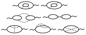
Figure 1: Non-RPA contributions into optical conductivity from the two-pair channel. Dashed line stands for the electron-electron interaction. The last three diagrams originate from exchange processes.

Derivation. Instead of calculating the real part of the optical conductivity directly from the set of diagrams of Fig. 1, we employ an equivalent and arguably more transparent method. Namely, we identify various processes leading to absorption (and emission) in the two-particle channel and calculate their transition probabilities using the Golden rule formalism Mishch . In diagrammatic terms, these various processes correspond to all possible cuts of the diagrams, Fig. 1, across any four fermion lines.

We begin with calculating transition rates between different two-particle states. The two-particle wave function is given by the Slater determinant,

$$\psi^{ab}_{\bf pk}({\bf x}_{1},{\bf x}_{2})=\frac{1}{\sqrt{2}}\left[\psi^{a}_{\bf p}({\bf x}_{1})\psi^{b}_{\bf k}({\bf x}_{2})-\psi^{a}_{\bf p}({\bf x}_{2})\psi^{b}_{\bf k}({\bf x}_{1})\right].$$ (3)

Here $\psi^{a}_{\bf p}({\bf x})$ is a single-particle wave function with the momentum ${\bf p}$ belonging to the $a$-th spin subband, $a=\pm 1$; the notation ${\bf x}$ stands for the in-plane coordinates, ${\bf x}=(x,y)$. For the “Rashba” coupling the eigenstates are

$$\psi^{a}_{\bf p}({\bf x})=\frac{1}{\sqrt{2}}\left(\begin{array}[]{c}e^{i\chi_{\bf p}/2}\\ ae^{-i\chi_{\bf p}/2}\end{array}\right)e^{i{\bf p\cdot x}/\hbar},$$ (4)

where $\chi_{\bf p}$ denotes the angle between the momentum ${\bf p}$ and the $y$-axis. The energy of these eigenstates is

$$\epsilon^{a}_{{\bf p}}={p^{2}}/{2m}+a\lambda p.$$ (5)

It is now necessary to calculate the probability of a transition from a state $\psi^{ab}_{\bf pk}$ into another state $\psi^{cd}_{\bf p^{\prime}k^{\prime}}$ in the presence of both the electron-electron interaction $V({\bf x_{1}}-{\bf x_{2}})$ and the electric field, which is described by a scalar potential,

$$\phi({\bf x},t)=\phi_{0}e^{-i\omega t+i{\bf q\cdot x}}+\phi_{0}^{*}e^{i\omega t-i{\bf q\cdot x}}.$$ (6)

Coupling of electrons to the external field (6) as well as the electron-electron interaction are treated in the second-order perturbation theory. Spin-orbit coupling, on the other hand, is not assumed to be small for the time being. Transition probability between different two-particle states, accompanied by the absorption of the energy $\omega$ from the external field, has the following form,

$$dW^{ab\to cd}_{{\bf pk}\to{\bf p^{\prime}k^{\prime}}}=2\pi e^{2}|\phi_{0}|^{2}\delta(\epsilon^{a}_{\bf p}+\epsilon^{b}_{\bf k}-\epsilon^{c}_{\bf p^{\prime}}-\epsilon^{d}_{\bf k^{\prime}}+\omega)$$

$$\times|\sum_{f}{\cal M}_{f}|^{2}\delta({\bf p}+{\bf k}-{\bf p^{\prime}}-{\bf k^{\prime}}+{\bf q})\frac{d^{2}p^{\prime}d^{2}k^{\prime}}{(2\pi)^{2}}.$$ (7)

where ${\cal M}_{f}$ is the amplitude for the transitions that occur via virtual states belonging to a subband $f$,

$${\cal M}_{f}=\frac{{\cal A}^{af}_{\bf p,p+q}\Bigl{(}{\cal A}^{fc}_{\bf p+q,p^{\prime}}V_{\bf k-k^{\prime}}{\cal A}^{bd}_{\bf k,k^{\prime}}-{\cal A}^{fd}_{\bf p+q,k^{\prime}}V_{\bf p^{\prime}-k}{\cal A}^{bc}_{\bf k,p^{\prime}}\Bigr{)}}{\epsilon^{a}_{\bf p}-\epsilon^{f}_{\bf p+q}+\omega}+\frac{\Bigl{(}{\cal A}^{af}_{\bf p,p^{\prime}-q}V_{\bf k-k^{\prime}}{\cal A}^{bd}_{\bf k,k^{\prime}}-{\cal A}^{ad}_{\bf p,k^{\prime}}V_{\bf p-k^{\prime}}{\cal A}^{bf}_{\bf k,p^{\prime}-q}\Bigr{)}{\cal A}^{fc}_{\bf p^{\prime}-q,p^{\prime}}}{\epsilon^{c}_{\bf p^{\prime}}-\epsilon^{f}_{\bf p^{\prime}-q}-\omega}$$

$$+\frac{{\cal A}^{bf}_{\bf k,k+q}\Bigl{(}{\cal A}^{ac}_{\bf p,p^{\prime}}V_{\bf p^{\prime}-p}{\cal A}^{fd}_{\bf k+q,k^{\prime}}-{\cal A}^{ad}_{\bf p,k^{\prime}}V_{\bf p-k^{\prime}}{\cal A}^{fc}_{\bf k+q,p^{\prime}}\Bigr{)}}{\epsilon^{b}_{\bf k}-\epsilon^{f}_{\bf k+q}+\omega}+\frac{\Bigl{(}{\cal A}^{ac}_{\bf p,p^{\prime}}V_{\bf p-p^{\prime}}{\cal A}^{bf}_{\bf k,k^{\prime}-q}-{\cal A}^{af}_{\bf p,k^{\prime}-q}V_{\bf p^{\prime}-k}{\cal A}^{bc}_{\bf k,p^{\prime}}\Bigr{)}{\cal A}^{fd}_{\bf k^{\prime}-q,k^{\prime}}}{\epsilon^{d}_{\bf k^{\prime}}-\epsilon^{f}_{\bf k^{\prime}-q}-\omega}.$$ (8)

Here $V_{\bf p-p^{\prime}}$ stands for the Fourier transform of the interaction potential, the notation ${\cal A}^{ac}_{\bf p,p^{\prime}}$ is used for the overlap of spin wave functions of single-electron states (4) before ($\psi^{a}_{\bf p}$) and after ($\psi^{c}_{\bf p^{\prime}}$) the scattering:

$${\cal A}^{ac}_{\bf p,p^{\prime}}=\frac{1}{2}\left(e^{i(\chi_{\bf p}-\chi_{\bf p^{\prime}})/2}+ac~{}e^{-i(\chi_{\bf p}-\chi_{\bf p^{\prime}})/2}\right).$$ (9)

The origin of various terms in the transition probability (Optical Conductivity of a 2D Electron Liquid with Spin-Orbit Interaction)-(Optical Conductivity of a 2D Electron Liquid with Spin-Orbit Interaction) is graphically represented in Fig. 2a).

The knowledge of transition probabilities allows one to find the rate at which the electron system absorbs energy from the external field (6). Taking into account the population of the electronic states, the energy absorption rate can be written as the sum over initial and final states,

$$I_{\rm abs}=\frac{\omega}{4}\sum_{abcd}\int\frac{d^{2}pd^{2}k}{(2\pi)^{4}}~{}dW^{ab\to cd}_{{\bf pk}\to{\bf p^{\prime}k^{\prime}}}n^{a}_{p}n^{b}_{k}(1-n^{c}_{p^{\prime}})(1-n^{d}_{k^{\prime}}).\\$$

Here $n^{a}_{p}$ is the Fermi-Dirac distribution for the $a$-th subband; the coefficient ${1}/{4}$ prevents double-counting of the initial and final states. The rate of emission of energy, $I_{\rm em}$ is most simply found from the detailed balance principle LLVIII , $I_{\rm em}=I_{\rm abs}e^{-\omega/T}$. The energy dissipation rate $I_{\rm abs}-I_{\rm em}$ can then be related to the real part of the optical conductivity at finite $q$,

$$\sigma^{\prime}(\omega,q)=\frac{(1-e^{-\omega/T})I_{\rm abs}}{2q^{2}|\phi_{0}|^{2}}.$$ (10)

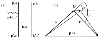
Figure 2: a) Graphic representation of the two-electron absorption amplitude ${\cal M}_{f}$, see Eq. (Optical Conductivity of a 2D Electron Liquid with Spin-Orbit Interaction). The wavy line (external electric field) can be inserted in four different ways (not shown here). In addition, interchange of the final states $c{\bf p^{\prime}}\leftrightarrow d{\bf k^{\prime}}$ yields four exchange terms, leading to the total of eight different terms in Eq. (Optical Conductivity of a 2D Electron Liquid with Spin-Orbit Interaction). Propagators of the virtual states result in the energy denominators. Each vertex brings a factor ${\cal A}^{ac}_{\bf p,k}$, where ${\bf p},a$ and ${\bf k},c$ are the incoming and outgoing electron momenta and subband indices, respectively. b) Electron momenta prior ${\bf p}$, ${\bf k}$ and after ${\bf p}+{\bf Q}$, ${\bf k}-{\bf Q}$ a collision. The angle of incidence between momenta ${\bf p}$ and ${\bf k}$ is denoted by $\theta$, and the angle of scattering between ${\bf p}$ and ${\bf Q}$ by $\phi$.

The general form of the optical conductivity $\sigma^{\prime}(\omega,q)$ is too cumbersome to analyze here, so we concentrate on the most interesting, homogeneous, limit, $\sigma^{\prime}(\omega)=\sigma^{\prime}(\omega,q\to 0)$. When taking the limit $q\to 0$ it is helpful to note that the matrix (9) reduces to the Kronecker symbol for coinciding momenta. The matrix element ${\cal M}_{f}$ thus vanishes in this limit, as required by the presence of $q^{2}$ in the denominator of Eq. (10). We emphasize the appearance of terms linear in $q$, which are due to spin-orbit interaction. When the latter is absent, the interference between the four terms in the absorption amplitude (Optical Conductivity of a 2D Electron Liquid with Spin-Orbit Interaction) leads to the cancelation of the linear terms and the vanishing of $\sigma_{2}(\omega)$ Mishch . To expand Eq. (Optical Conductivity of a 2D Electron Liquid with Spin-Orbit Interaction) to the linear order in $q$, we note that only the denominators need to be expanded, as the expansion of the numerators leads only to small corrections. As a result, we obtain,

$$\sigma^{\prime}_{2}(\omega) = e^{2}\frac{\lambda^{2}(1-e^{-{\omega}/{T}})}{16\omega^{3}}\sum_{abcd}\int\frac{d^{2}pd^{2}kd^{2}p^{\prime}d^{2}k^{\prime}}{(2\pi\hbar)^{5}}\Big{|}{\cal A}^{ac}_{\bf p,p^{\prime}}{\cal A}^{bd}_{\bf k,k^{\prime}}V_{\bf k-k^{\prime}}-{\cal A}^{ad}_{\bf p,k^{\prime}}{\cal A}^{bc}_{\bf k,p^{\prime}}V_{\bf p^{\prime}-k}\Big{|}^{2}n^{a}_{p}n^{b}_{k}(1-n^{c}_{p^{\prime}})(1-n^{d}_{k^{\prime}})$$ (11)

$$\times\Bigl{(}a~{}{\bf n}_{\bf p}+b~{}{\bf n}_{\bf k}-c~{}{\bf n}_{\bf p^{\prime}}-d~{}{\bf n}_{\bf k^{\prime}}\Bigr{)}^{2}\delta(\epsilon^{a}_{\bf p}+\epsilon^{b}_{\bf k}-\epsilon^{c}_{\bf p^{\prime}}-\epsilon^{d}_{\bf k^{\prime}}+\hbar\omega)\delta({\bf p}+{\bf k}-{\bf p^{\prime}}-{\bf k^{\prime}}),$$

where ${\bf n}_{\bf p}$ is the unit vector in the direction ${\bf p}$. As seen from its form, this result is due to the interplay of spin-orbit coupling and electron-electron interaction.

To proceed further, we utilize the fact that spin-orbit coupling is typically small, $m\lambda\ll p_{F}$. Since the homogeneous optical conductivity (11) is already proportional to $\lambda^{2}$, in the leading order it is sufficient to take the limit $\lambda\to 0$ in the delta-function and Fermi-Dirac distributions in the integrand of Eq. (11). The summation over the subband indices can then be easily carried out,

$$\sigma^{\prime}_{2}(\omega)=e^{2}\frac{\lambda^{2}(1-e^{-{\omega}/{T}})}{2\omega^{3}}\int\frac{d^{2}pd^{2}kd^{2}Q}{(2\pi)^{5}}{\cal P}({\bf p,k,Q})$$

$$\times n_{p}n_{k}(1-n_{p})(1-n_{k^{\prime}})\delta(\epsilon_{p}+\epsilon_{k}-\epsilon_{p^{\prime}}-\epsilon_{k^{\prime}}+\hbar\omega).~{}~{}$$ (12)

Here we integrated out the momentum delta-function by introducing explicitly the momentum of electron-hole pairs, ${\bf Q}={\bf p^{\prime}}-{\bf p}={\bf k}-{\bf k^{\prime}}$. The explicit expression for the probability of inelastic collisions ${\cal P}({\bf p,k,Q})$ is simple but rather lengthy. In the simplest case of screened (e.g. by a metallic gate) short-range interaction $V_{q}=V$ this probability is given by ${\cal P}({\bf p,k,Q})=V^{2}[2-({\bf n}_{\bf p}\cdot{\bf n_{k}})^{2}-({\bf n}_{\bf p^{\prime}}\cdot{\bf n}_{\bf k^{\prime}})^{2}]$. In order to evaluate the integrals in Eq. (Optical Conductivity of a 2D Electron Liquid with Spin-Orbit Interaction), it is convenient to make use of the variables $\xi_{p},\xi_{k},Q,\theta,\phi$, where $\xi_{p}=(p^{2}-p_{F}^{2})/2m$, and the choice of angles $\theta$ and $\phi$ is illustrated by Fig. 2b). Then $d^{2}pd^{2}kd^{2}Q=2(2\pi)m^{2}d\xi_{p}d\xi_{k}QdQd\theta d\phi$; here the extra factor $2$ comes from the processes that differ from those shown in Fig. 2b) by rotating vectors ${\bf p^{\prime}}$, ${\bf k^{\prime}}$ around the direction of the vector ${\bf p}+{\bf k}$ by the angle $\pi$.

If $\omega,T\ll p^{2}_{F}/2m$, the characteristic momenta of electron-hole pairs, $Q\sim\max(\omega,T)/v_{F}$, are much smaller than the Fermi momentum $p_{F}$. Thus, we can approximate ${\cal P}\approx 2V^{2}\sin^{2}\theta$. The argument of the delta-function in this limit, $\omega-Qv_{F}\cos\phi+Qv_{F}\cos(\theta-\phi)$, is independent of $\xi_{p}$ and $\xi_{k}$. This makes it possible to perform integration over $d\xi_{p}d\xi_{k}$ first. The integral over $dQ$ then removes the delta-function. Resulting angle integrals cannot be calculated analytically for arbitrary temperatures. However, two important limits, $\omega\gg\pi T$ and $\omega\ll\pi T$, can be easily analyzed. After some straightforward calculations we arrive at Eq. (2).

Long-range interaction. Let us now address the case of a long-range RPA Coulomb interaction which we consider here for the $T=0$ limit only. The interaction can be written with the help of the usual dimensionless parameter $r_{s}=\sqrt{2}me^{2}/(p_{F}\varepsilon)$, as $V_{\bf k}=\sqrt{2}\pi r_{s}v_{F}/(|{\bf k}|+\sqrt{2}r_{s}p_{F})$; here $\varepsilon$ is the dielectric constant. The scattering probability can now be approximated with clarification ,

$${\cal P}\approx\frac{2\pi^{2}r_{s}^{2}\sin^{2}{\theta}}{m^{2}(\sqrt{1-\cos{\theta}}+r_{s})^{2}}.$$

The angle integrals can be performed numerically; dependence of $\sigma^{\prime}_{2}$ on the electronic density is shown in Fig. 3.

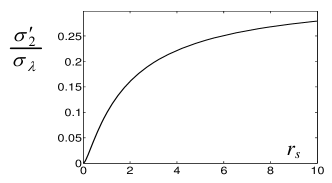
Figure 3: Dependence of the many-body optical conductivity, measured in units of $\sigma_{\lambda}=e^{2}\lambda^{2}/(2\pi v_{F})^{2}$, on the interaction parameter $r_{s}$ for long-range Coulomb interaction.

Discussion. Let us emphasize a number of important points concerning this result. At zero temperature, the many-body contribution $\sigma^{\prime}_{2}$ is $\sim\lambda^{2}/v_{F}^{2}$ times weaker than the one-particle Landau damping $\sigma^{\prime}_{1}$, but it has much broader spectrum. Also, in contrast to Landau damping $\sigma^{\prime}_{2}$, is enhanced with increasing the temperature. Note that when frequency decreases, $\omega\to 0$, and temperature is kept constant, $\sigma^{\prime}_{2}(\omega)$ diverges. This singularity s cut-off by the finite scattering rate $\tau^{-1}$ due to small amount of phonons (present for any finite $T$) or impurities.

The absence of a logarithm in the many-body optical conductivity is in a sharp contrast with other quantities describing properties of 2DEG, namely, quasiparticle lifetime Ch ; HSW ; JMD ; ZDS , Coulomb drag resistivity GEM , thermal conductivity LM ; CA , or finite-$q$ optical conductivity Mishch . This is a consequence of the vanishing of the amplitude ${\cal P}\propto\theta^{2}$ in Eq. (Optical Conductivity of a 2D Electron Liquid with Spin-Orbit Interaction) for almost collinear, $\theta\approx 0,\pi$, scattering processes. Indeed, as the corresponding scattering amplitudes are enhanced for such collinear processes, the logarithmic factor, typical for 2D, may be viewed as a “trace” of weakened one-dimensional singularities Chub . The problem analyzed in the present work, however, is inherently different. In one dimension the discussed effect would be absent. Despite the fact that spin-orbit coupling breaks Galilean invariance in 1D as well, spin-conserving nature of Coulomb interaction assures that electrons preserve their chirality (subband indices) during collisions. Thus, the interplay of spin-orbit coupling and interactions does not modify the optical conductivity of a one-dimensional electron system.

An important note should be made about exchange processes. Since it is the entire range of angles, $\theta\sim 1$, that contributes to the optical conductivity in 2DEG with spin-orbit coupling, and not simply the forward scattering domain, $\theta\approx 0$, the exchange processes are important. Therefore, all diagrams in Fig. 1 are relevant. This is different from a typical scenario when exchange processes are negligible provided that the density of carriers is high.

Summary and Conclusions. We have analyzed the many-body contribution to the optical conductivity of a two-dimensional electron liquid in the presence of spin-orbit coupling. The latter breaks Galilean invariance, making electron dispersion non-parabolic. This opens a possibility for optical conductivity to be used as a probe for many-body effects. This non-trivial interplay of spin-orbit coupling and electron-electron interactions was revealed here for the first-time. Experimental observation of the above effect can be performed in GaAs-based quantum wells as well as in 2D states on the vicinal surfaces (111) of noble metals noble ; noble1 . To eradicate extraneous electron scattering the measurements have to be performed on clean samples at low temperatures.

We acknowledge fruitful discussions with M. Raikh, M. Reizer, O. Starykh, A. Chubukov, and S. Gangadharaiah. The work was supported by the Department of Energy, Office of Basic Energy Sciences.

References

- (1) D. Pines and P. Nozieres, The Theory of Quantum Liquids (Benjamin, New York, 1966).
- (2) F.T. Vas’ko, JETP Lett. 30, 540 (1979); Yu.A. Bychkov and E.I. Rashba, J. Phys. C 17, 6039 (1984).
- (3) L.I. Magarill, A.V. Chaplik and M.V. Éntin, JETP 92, 153 (2001).
- (4) E.G. Mishchenko and B.I. Halperin, Phys. Rev. B 68, 045317 (2003).
- (5) E.I. Rashba and V.I. Sheka, in Landau Level Spectroscopy, edited by G. Landwehr and E.I. Rashba (North-Holland, Amsterdam, 1991), p. 131.
- (6) A. Shekhter, M. Khodas, and A.M. Finkelstein, Phys. Rev. B 71, 165329 (2005).
- (7) G.-H. Chen and M.E. Raikh, Phys. Rev. B 59, 5090 (1999).
- (8) E. G. Mishchenko, M. Yu. Reizer, and L. I. Glazman, Phys. Rev. B 69, 195302 (2004).
- (9) L.D. Landau and E.M. Lifshitz, Electrodynamics of Continuous Media (Pergamon, Oxford, 1984).
- (10) Note, that decreasing density (increasing ), also means decreasing transferred momentum, . Thus, the condition is satisfied with progressively better accuracy and the amplitude of scattering becomes effectively short-range (-independent).
- (11) A.V. Chaplik, Sov. Phys. JETP 33, 997 (1971).
- (12) C. Hodges, H. Smith and J.W. Wilkins, Phys. Rev. B 4, 302 (1971).
- (13) T. Jungwirth and A.H. MacDonald, Phys. Rev. B 53, 7403 (1996).
- (14) Lian Zheng and S. Das Sarma, Phys. Rev. B 53, 9964 (1996).
- (15) M. Kellog, J.P. Eisenstein, L.N. Pfeiffer and K.W. West, cond-mat/0206547.
- (16) A.O. Lyakhov and E.G. Mishchenko, Phys. Rev. B 67, 041304(R) (2003).
- (17) G. Catelani and I.L. Aleiner, JETP 100, 331 (2005).
- (18) A.V. Chubukov, D.L. Maslov, S. Gangadharaiah, and L.I. Glazman, Phys. Rev. B 71, 205112 (2005).
- (19) F.J. Himpsel, et al., Adv. Phys. 47, 511 (1998).
- (20) R. Nötzel, et al., Nature 392, 56 (1998); P. Segovia, et al., ibid. 402, 504 (1999); P. Gambardella, ibid. 416, 301 (2002).