Phase Diagram of the Holstein-Hubbard Two-Leg Ladder

Abstract

Using a functional renormalization group method, we obtain the phase diagram of the two-leg ladder system within the Holstein-Hubbard model, which includes both electron-electron and electron-phonon interactions. Our renormalization group technique allows us to analyze the problem for both weak and strong electron-phonon coupling. We show that, in contrast results from conventional weak coupling studies, electron-phonon interactions can dominate electron-electron interactions because of retardation effects.

The renormalization group (RG) method has provided fundamental understanding of the stable phases of matter in terms of the basin of attraction of fixed points (FP). Quantum phase transitions (QPT) between different fixed points can be described in terms of the stability of these FP relative to the RG flow. In the theory of metals, Landau’s Fermi liquid theory can be described either as a stable FP of the renormalization group flow under repulsive interactions, or as an unstable FP under attractive interactions to a superconducting state (SC) described by BCS theory Shankar . Apart from determining the stability of a FP, the RG method also provides direct information about the energy scales (gaps) and length scales (correlation lengths) associated with a QPT. Hence, the RG not only provides qualitative information, but also quantitative information, about the different phases of matter.

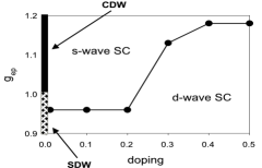
Figure 1: Phase diagram of Holstein-Hubbard ladder as a function of electron-phonon coupling $g_{\rm{ep}}$ and doping ($t=1$,$U=2$, $\omega_{0}=1$). Zero doping corresponds to half-filling and doping of 0.5 corresponds to quarter-filling.

In practice, however, there are very few examples of problems in which the RG can be implemented beyond weak coupling kondo . Furthermore, another well-known challenge to the RG has been its implementation in problems with retardation, such as the electron-phonon (e-ph) problem, because of the introduction of multiple, frequency-dependent interaction channels that renormalize in a collective, energy dependent, way. At weak e-ph coupling, when retardation plays a small role, the RG can be implemented using approximations such as the so-called ”two-step” RG Zimanyi ; Seidel . Usually, the two-step RG leads to an enhancement of the instabilities that exist when only electron-electron (e-e) interactions are present, but does not describe phases where retardation effects due to the e-ph coupling become dominant over e-e effects. In fact, we show that new phases, such as charge density wave (CDW) and s-wave SC, emerge at strong e-ph coupling (see Fig. 1).

Recently, the RG was extended to study the non-perturbative physics of the e-ph problem in the large $N$ limit (where $N=E_{F}/\Lambda$, $E_{F}$ is the Fermi energy and $\Lambda$ is the cut-off) in the presence of electron-electron (e-e) interactions for a two-dimensional circular (three-dimensional spherical) Fermi surface Tsai1 . In particular, that work established that the stable FP of this problem is described by the Eliashberg-Migdal theory, which contains BCS as its weak-coupling limit. Since it has few scattering channels Shankar , the circular (spherical) Fermi surface, which is a consequence of the plane-wave character of the electronic wavefunctions, is a particularly simple problem. This is not the case for Fermi surfaces that derive from localized electronic orbitals that can be either unstable to exotic SC (such as p- and d-wave) or to density wave (charge and spin) phases. Arguably, the most famous example of this phenomenon are the one-dimensional (1D) conductors where the nesting associated with Fermi points leads to a richness of phases that can be described by g-ology, bosonization Solyom ; vojt , and the functional RG Tam . However, the 1D problem is very particular because of the restricted phase space for interaction, and even in 1D, the treatment of the e-ph interaction is problematic vojt_phonons .

The recently developed e-ph coupled functional renormalization group (FRG) Tsai1 includes the merits of the FRG for the pure e-e interacting system Shankar ; Zanchi ; Halboth and goes beyond the two-step renormalization group for the e-ph interacting system Caron ; Zimanyi ; Seidel , by allowing the systematic study of the full frequency dependence of couplings. In this paper we use this newly extended FRG to study the two-leg ladder Holstein-Hubbard model that describes a quasi-1D system in the presence of e-e and e-ph interactions. The ladder system, consisting of two 1D chains coupled by inter-chain hopping, can be considered as an intermediate between 1D and 2D systems, since it shares properties with both: it has a limited number of scattering channels, as in 1D, but also can show SC with 2D characteristics, such as d-wave order parameter White ; Balents . As a result, ladders have been considered by many as a theoretical testbed for the understanding of high-Tc superconductivity rice .

Furthermore, the interest in the e-ph problem in high-Tc has been revitalized by experimental evidence that the e-ph coupling may play a critical role in these systems Lanzara ; Shen . Apart from the cuprates, ladder systems have also attracted much attention recently because, from the technical point of view, they are amenable to field theoretical calculations and to reliable numerical simulations, in contrast to truly 2D systems. Studying the interplay between the e-e and e-ph interactions in a ladder is also important for the understanding the physics of some low-dimensional materials, such as molecular crystals and charge transfer solids Organics .

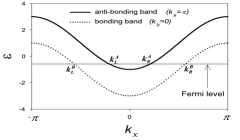
Figure 2: Energy dispersion for free electrons in a 2-leg ladder.

The Holstein-Hubbard model (HHM) is described by the following Hamiltonian (we use units such that $\hbar=1=k_{B}$):

$$H = -t\sum_{\langle i,j\rangle,\sigma}(c_{i,\sigma}^{\dagger}c_{j,\sigma}+H.c.)+U\sum_{i}n_{i,\uparrow}n_{i,\downarrow}$$ (1)

$$+g_{\rm{ep}}\sum_{i,\sigma}(a_{i}^{\dagger}+a_{i})n_{i,\sigma}+\omega_{0}\sum_{i}a_{i}^{\dagger}a_{i}\,,$$

where $c_{i,\sigma}^{\dagger}$ ($c_{i,\sigma}$) creates (annihilates) an electron at site $i$ with spin $\sigma$ ($n_{i\sigma}$ is the electron number operator), $a_{i}^{\dagger}$ ($a_{i}$) creates (annihilates) an optical phonon at site $i$ with energy $\omega_{0}$, $t$ is the hopping energy of the electrons along legs and rungs of the ladder, $U$ is the on-site e-e interaction, and $g_{\rm{ep}}$ is the e-ph coupling energy. In the absence of e-e ($U=0$) and e-ph ($g_{\rm{ep}}=0$) interactions, the energy spectrum of the electrons has the form shown in Fig. 2. In what follows we use units such that $t=1$.

One can reformulate the problem in terms of path integrals, and since the phonon fields enter quadratically in the action, they can be integrated out exactly Tsai1 , generating an effective action $S$ for the electrons that can be written as:

$$S = \int_{\underline{k},\sigma}\psi^{\dagger}_{\sigma}(\underline{k})(i\omega-\epsilon_{k})\psi_{\sigma}(\underline{k})$$

$$+ \int_{\{\underline{k}\},\sigma,\sigma^{{}^{\prime}}}g(\underline{k_{1}},\underline{k_{2}},\underline{k_{3}},\underline{k_{4}})\psi^{\dagger}_{\sigma}(\underline{k_{4}})\psi^{\dagger}_{\sigma^{{}^{\prime}}}(\underline{k_{3}})\psi_{\sigma^{{}^{\prime}}}(\underline{k_{2}})\psi_{\sigma}(\underline{k_{1}}),$$

where $\psi$ is the electron field, and the coupling functions for electron-electron interactions in the momentum space are given by:

$$g(\underline{k_{1}},\underline{k_{2}},\underline{k_{3}},\underline{k_{4}})=U-2g_{\rm{ep}}^{2}\omega_{0}/[\omega_{0}^{2}+(\omega_{1}-\omega_{4})^{2}],$$ (3)

where $\underline{k}=(k,\omega)$. Each coupling is a function of the in-coming and out-going momenta and frequencies, subjected to the conservation of momenta, $k_{1}+k_{2}=k_{3}+k_{4}$ and energy $\omega_{1}+\omega_{2}=\omega_{3}+\omega_{4}$. In a purely e-e interacting system, the coupling functions are always independent of the frequency. For a generic system with e-ph interactions, the couplings become frequency dependent, i.e., retarded. We choose $g(\underline{k_{1}},\underline{k_{2}},\underline{k_{3}},\underline{k_{4}})$ to represent the scattering between electrons with opposite spins. The coupling functions for scattering between electrons with parallel spins are determined by those with opposite spin due to the SU(2) spin symmetry.

Following ref. [Tsai1, ], our only assumption is that the full bandwidth of the two-leg ladder system is larger than any of the interaction terms: i.e., that $6t\gg U,g_{\rm{ep}},\omega_{0}$, leaving the relative values of $U$, $\omega_{0}$ and $g_{\rm{ep}}$, free. The strong coupling limit of the electron-phonon problem occurs when $\lambda\equiv 2N(0)g_{\rm{ep}}^{2}/\omega_{0}\gg 1$. This regime is accessible in our functional RG approach. Utilizing the time-reversal symmetry, exchange symmetry, and reflection symmetry, the number of independent couplings in the Fermi surface for the 2-leg ladder at incommensurate fillings is 12 (each coupling is a function of three momenta and three frequencies, the frequency dependences are suppressed for clarity). There are 6 intra-band couplings:

$$g_{4}^{A}=g(k_{L}^{A},k_{L}^{A},k_{L}^{A},k_{L}^{A}), g_{4}^{B}=g(k_{L}^{B},k_{L}^{B},k_{L}^{B},k_{L}^{B}),$$

$$g_{1}^{A}=g(k_{L}^{A},k_{R}^{A},k_{L}^{A},k_{R}^{A}), g_{1}^{B}=g(k_{L}^{B},k_{R}^{B},k_{L}^{B},k_{R}^{B}),$$

$$g_{2}^{A}=g(k_{L}^{A},k_{R}^{A},k_{R}^{A},k_{L}^{A}), g_{2}^{B}=g(k_{L}^{B},k_{R}^{B},k_{R}^{B},k_{L}^{B});$$ (4)

and 6 inter-band couplings:

$$g_{1}^{C}=g(k_{L}^{A},k_{L}^{B},k_{L}^{A},k_{L}^{B}), g_{2}^{C}=g(k_{L}^{A},k_{L}^{B},k_{L}^{B},k_{L}^{A}),$$

$$g_{1}^{D}=g(k_{L}^{B},k_{R}^{B},k_{L}^{A},k_{R}^{A}), g_{2}^{D}=g(k_{L}^{B},k_{R}^{B},k_{R}^{A},k_{L}^{A}),$$

$$g_{1}^{E}=g(k_{L}^{B},k_{R}^{A},k_{L}^{B},k_{R}^{A}), g_{2}^{E}=g(k_{L}^{B},k_{R}^{A},k_{R}^{A},k_{L}^{B}).$$ (5)

For pure e-e interactions the Fermi velocities are renormalized by $g_{4}^{A}$ and $g_{4}^{B}$, and the renormalizations of scattering between particles on the same side of the Brillouin zone at different bands, $g_{1}^{C}$ and $g_{2}^{C}$, are absent in the leading order. This is not necessarily valid for couplings with frequency dependence. Moreover, these couplings generate self-energy corrections, which have been shown to be important for studying the system with retardation effects Tsai1 , leading to the renormalization of Fermi velocities and quasiparticle lifetime. Thus we keep these couplings even though they are not renormalized in the non-retarded system . In leading order, our renormalization group equations for the coupling function, $g_{\Lambda}(\underline{k}_{1},\underline{k}_{2},\underline{k}_{3})$, and for the self-energy, $\Sigma_{\Lambda}(\underline{k})$, are given by:

$$\partial_{\Lambda}g_{\Lambda}(\underline{k_{1}},\!\underline{k_{2}},\!\underline{k_{3}})=$$ (6)

$$- \!\!\!\!\int\!d\underline{p}\partial_{\Lambda}\![G_{\Lambda}(\underline{p})G_{\Lambda}(\underline{k})]g_{\Lambda}(\underline{k_{1}},\!\underline{k_{2}},\!\underline{k})g_{\Lambda}(\underline{p},\!\underline{k},\!\underline{k_{3}})$$

$$- \!\!\!\!\int\!d\underline{p}\partial_{\Lambda}\![G_{\Lambda}(\underline{p})G_{\Lambda}(\underline{q_{1}})]g_{\Lambda}(\underline{p},\!\underline{k_{2}},\!\underline{q_{1}})g_{\Lambda}(\underline{k_{1}},\!\underline{q_{1}},\!\underline{k_{3}})$$

$$- \!\!\!\!\int\!d\underline{p}\partial_{\Lambda}\![G_{\Lambda}(\underline{p})G_{\Lambda}(\underline{q_{2}})][-\!2g_{\Lambda}(\underline{k_{1}},\!\underline{p},\!\underline{q_{2}})g_{\Lambda}(\underline{q_{2}},\!\underline{k_{2}},\!\underline{k_{3}})$$

$$+ \!\!g_{\Lambda}\!(\underline{p},\!\underline{k_{1}},\!\underline{q_{2}})\!g_{\Lambda}\!(\underline{q_{2}},\!\underline{k_{2}},\!\underline{k_{3}})\!\!+\!g_{\Lambda}\!(\underline{k_{1}},\!\underline{p},\!\underline{q_{2}})g_{\Lambda}\!(\underline{k_{2}},\!\underline{q_{2}},\!\underline{k_{3}})],$$

$$\partial_{\Lambda}\Sigma_{\Lambda}(\underline{k})\!=\!-\!\!\!\int\!d\underline{p}\partial_{\Lambda}[G_{\Lambda}(\underline{p})][2g_{\Lambda}(\underline{p},\underline{k},\underline{k})\!-\!g_{\Lambda}(\underline{k},\underline{p},\underline{k})],$$ (7)

where $\underline{k}=\underline{k_{1}}+\underline{k_{2}}-\underline{p}$, $\underline{q_{1}}=\underline{p}+\underline{k_{3}}-\underline{k_{1}}$, $\underline{q_{2}}=\underline{p}+\underline{k_{3}}-\underline{k_{2}}$, $\int d\underline{p}=\int dp\sum_{\omega}1/(2\pi\beta)$, and $G_{\Lambda}$ is the self-energy corrected propagator at cutoff $\Lambda$. The initial condition for the coupling functions is given by (3). The self-energies are equal to zero at $\Lambda=\Lambda_{0}$.

For a non-retarded system the low energy instability can be obtained from the RG flow of the couplings, and different phases can be identified by the FP corresponding to the different spin and charge modes. This procedure may not be appropriate for system with electron-phonon coupling. Numerical evidence indicates that the half-filled Holstein-Hubbard model violates the Luttinger relations Tezuka . Therefore, instead of following the flows of the couplings, we explicitly construct the flows of the susceptibilities of different order parameters to obtain a unbiased answer within the FRG. The SC susceptibility, $\chi^{\delta}(k,\omega)$, is defined as:

$$\chi^{\delta}_{\Lambda}(0,0)\!\!=\!\!\int\!\!D(1,2)f^{\delta}(p_{1})f^{\delta}(p_{2})\langle c_{p_{1},\downarrow}c_{-p_{1},\uparrow}c_{-p_{2},\uparrow}^{\dagger}c_{p_{2},\downarrow}^{\dagger}\rangle\!,$$ (8)

where $\delta=s,d$ for s- and d-wave SC, respectively com . The RG equations are:

$$\partial_{\Lambda}\chi^{\delta}_{\Lambda}(0,0)=\int d\underline{p}\partial_{\Lambda}[G_{\Lambda}(\underline{p})G_{\Lambda}(-\underline{p})](Z^{\delta}_{\Lambda}(\underline{p}))^{2},$$ (9)

$$\partial_{\Lambda}\!Z^{\delta}_{\Lambda}\!(\underline{p})\!\!=\!\!-\!\!\!\int\!\!\!d\underline{p}^{\prime}\!\partial_{\Lambda}\![G_{\Lambda}\!(\underline{p}^{\prime})G_{\Lambda}\!(\!-\underline{p}^{\prime})\!]\!Z^{\delta}_{\Lambda}\!(\underline{p^{\prime}})g_{\Lambda}\!(\underline{p^{\prime}}\!,\!\!-\underline{p^{\prime}},\!\!-\underline{p},\!\underline{p})\!.$$ (10)

The function $Z_{\Lambda}^{\delta}(\underline{p})$ is the effective vertex in the definition for the susceptibility $\chi_{\Lambda}^{\delta}$. Its initial condition, at $\Lambda=\Lambda_{0}$, is $1$ for s-wave pairing and $cos(k_{x})-cos(k_{y})$ for d-wave pairing. The RG equations for susceptibilities are solved with initial condition $\chi^{\delta}_{\Lambda=\Lambda_{0}}(0,0)=0$. The dominant instability in the ground state is given by the most divergent susceptibility by solving the RG equations numerically. In the calculations reported here, we have discretized the frequency axis into 9 points and have checked that our results are essentially unchanged when additional discretization points are added.

Without e-ph coupling the d-wave pairing is the generic dominant instability for $0$ to $0.5$ doping (half- to quarter-filled), except in a narrow region in the parameter space where all the charge and spin degrees of freedom are gapless. The large region of d-wave pairing in the ladder comes from the anisotropy between the transverse and the parallel directions, which leads the pair scattering to develop a directional dependence when the high energy degrees of freedom are eliminated. For the Holstein coupling, the phonon-mediated attractive retarded interaction is independent of the momentum transfer and is thus isotropic. The attractive interaction is relevant in generating pair-scattering, since it leads the particle-particle ladder diagrams to acquire logarithmic divergences. The d-wave pairing from repulsive interaction does not come from this divergence, and thus the attractive interaction is very effective in leading the pairing instability, and more importantly, this pairing has s-wave symmetry. Therefore, the e-ph coupling tends to enhance the s-wave component in the pairing scattering matrix, and once this coupling exceeds a critical value, the s-wave susceptibility overcomes the d-wave, causing a transition from d- to s-wave SC pairing symmetry. This result can only be seen in strong coupling and, hence, is not accessible to the two-step RG Seidel . A study of the fully retarded problem for a 2D circular Fermi surface has similarly shown how the two-step RG breaks down in the strong coupling ($\lambda\gg 1$) limit Tsai2 .

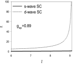
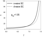
Figure 3: The flows of s-wave SC (solid lines), and d-wave SC (dotted lines) susceptibilities as a function of $l=\ln(\Lambda_{0}/\Lambda)$ for $U=2$, $\omega_{0}=1$, and doping of $0.2$.

In Fig. 3 we show a representative RG flow in which we observe the change in the dominant susceptibility for increasing e-ph coupling $g_{\rm{ep}}$. Although the isotropic phonons tend to break the d-wave pairs, as long as the e-ph coupling is small compared to the e-e interactions, the d-wave pairing remains the dominant instability. However, the s-wave overcomes the d-wave pairing when the effective interaction in the anti-adiabatic limit, $U_{{\rm effective}}=U-2g_{\rm{ep}}^{2}/\omega_{0}$, is near zero. As the doping increases, the critical values for the pairing transition remain close to the points where the anti-adiabatic effective interaction vanishes. Notice that for a ladder, the d-wave SC region increases with doping and is rather stable against s-wave near quarter filling, because the Fermi surface becomes more anisotropic with doping. This result should be contrasted with the 2D case where d-wave superconductivity seems to be suppressed at larger doping because the Fermi surface becomes more isotropic. Hence, our results show that one has to be cautious when comparing results for ladders with the true 2D problem. For doping close to the quarter filling, we find noticeable changes in the critical values, and a substantially stronger electron-phonon interaction is needed to drive the s-wave pairing over the d-wave pairing. This can be understood from the fact that the difference between the Fermi velocities of the anti-bonding and bonding bands becomes larger as the system is doped away from half-filling (see Fig. 2). From the perspective of the Fermi surface renormalization group, this difference leads to different contributions to pair scattering at $k_{y}=0$ and at $k_{y}=\pi$, which in turn lead to a phase difference in the pairing matrix elements which is manifested as a d-wave pairing channel. This is the reason that the d-wave channel becomes stronger as the doping gets closer to quarter filling. Nevertheless, the s-wave remains still the dominant instability for sufficiently strong e-ph coupling.

Exactly at quarter filling, the Fermi surface in the anti-bonding band shrinks to a point, which leads to a van Hove singularity at the center of the anti-bonding band. Also, at this filling the distance between the Fermi points in the bonding band is commensurate, which results in the presence of an extra Umklapp scattering in the bonding band, $g_{3}^{B}=(k^{B}_{L},k^{B}_{L},k^{B}_{R},k^{B}_{R})$. We do not find that the Umklapp scattering is sufficient to drive the system to spin density wave (SDW) phase. In contrast to the case without phonons $\lambda=0$ Balents we do not find a Luttinger liquid phase (C2S2). The d-wave pairing is still the dominant instability for small e-ph coupling, and the s-wave again overcomes the d-wave at strong coupling. Below quarter filling, the anti-bonding band is empty. Only two Fermi points remain on the bonding band. The system becomes essentially 1D as the effect of the anti-bonding band is then irrelevant.

We have also investigated the problem exactly at half-filling. In this particular commensurate doping there is a direct competition between a SDW and a CDW phase. In the absence of e-ph interaction the SDW phase (with a charge gap but no spin gap) is very robust and is not destabilized at weak coupling. At intermediate coupling ($\lambda\approx 1$), however. the SDW phase becomes unstable to a CDW phase with a charge gap. This result cannot be obtained in the weak coupling methods discussed previously.

The final results of our study are summarized in the phase diagram of Fig. 1. We find that the e-ph coupling at intermediate and strong coupling leads to substantial qualitative differences from previous results, including the appearance of new phases: CDW and s-wave SC. Moreover, we see that the d-wave phase is stabilized close to quarter filling, in contrast with the 2D case.

In conclusion, we have studied the effect of e-ph coupling on the phase diagram of a two-leg ladder, using the Holstein-Hubbard model and applying the functional renormalization group method. This method deals with the retardation effects in a systematic way. In particular, when the e-ph interaction strength is comparable to the e-e interactions and $\lambda\gg 1$, there are qualitative differences in the phase diagram from that predicted in previous studies. In particular, in addition to the SDW and d-wave SC phases found previously, we establish that for strong e-ph coupling, both CDW and s-wave SC can arise.

A.H.C.N. was supported through NSF grant DMR-0343790.

References

- (1) R. Shankar, Rev. Mod. Phys. 66, 129 (1994).
- (2) Famous counter examples to this rule include the class of impurity problems such as the Kondo problem. See, for instance, K. G. Wilson, Rev. Mod. Phys. 47, 773 (1975).
- (3) G. T. Zimanyi et al., Phys. Rev. Lett. 60, 2089 (1998).
- (4) A. Seidel et al., Phys. Rev. B 71, 220501 (R) (2005).
- (5) S.-W. Tsai et al., Phys. Rev. B 72, 054531 (2005).
- (6) J. Sólyom, Adv. Phys. 28, 201 (1979).
- (7) J. Voit, Rep. Prog. Phys. 58, 977 (1995).
- (8) K.-M. Tam et al., Phys. Rev. Let. 96, 036408 (2006).
- (9) J. Voit and H. J. Schulz, Phys. Rev. B 37, 10068 (1988).
- (10) D. Zanchi and H. J. Schulz, Phys. Rev. B 61, 13609 (2000).
- (11) C. J. Halboth and W. Metzner, Phys. Rev. B 61, 7364 (2000).
- (12) L. G. Caron and C. Bourbonnais, Phys. Rev. B 29, 4230 (1984).
- (13) S. R. White and D. J. Scalapino, Phys. Rev. Lett. 81, 3227 (1998).
- (14) L. Balents and M. P. A. Fisher, Phys. Rev. B 53, 12133 (1996); H.-H. Lin et al., Phys. Rev. B 56, 6569 (1997).
- (15) See, for instance, E. Dagotto, and T. M. Rice, Science 271, 618 (1996), and references therein.
- (16) A. Lanzara et al., Nature (London) 412, 510 (2001).
- (17) Z.-X. Shen et al., Philos. Mag. B 82, 1349 (2002).
- (18) T. Ishiguro and K. Yamaji, Organic Superconductors (Springer-Verlag, Berlin, 1990).
- (19) M. Tezuka et al., Phys. Rev. Lett. 95, 226401 (2005).
- (20) , is the Jacobian for the coordinate transformation from to , , and .
- (21) S.-W. Tsai et al, cond-mat/0505426.