Nonlinear optical response and exciton dephasing
in quantum dots

Abstract.

The full time-dependent four-wave mixing polarization in quantum dots is microscopically calculated, taking into account acoustic phonon-assisted transitions between different exciton states of the dot. It is shown that quite different dephasing times of higher exciton states in pancake anisotropic InGaAs quantum dots are responsible for the experimentally observed [1] double-exponential decay in the photon echo signal.

1. Introduction

Dephasing of the optical polarization caused by the interaction with lattice vibrations (phonons) is inevitable in solid state nanostructures and presents a fundamental obstacle for their application in quantum computing. Exciton dephasing in InGaAs quantum dots (QDs) has been recently studied by time-integrated four-wave mixing (FWM) measurements [2]. For the ground state excitonic transition in QDs, the temporal dynamics of the measured nonlinear polarization shows an initial rapid decay within the first few picoseconds which is followed at later times by a much slower exponential decay of the zero-phonon line [2, 3]. Excited states, in turn, have a quite different behavior. It has been recently shown [1] that after an initial fast decay (similar to that of the ground state) the excited state polarization has a double-exponential decay. A related non-exponential long-time decay has been also observed in QD molecules [4].

The initial decay has been studied theoretically by Vagov et al. [5, 6], taking into account the interaction of a single exciton state of a QD with bulk acoustic phonons, and using the exactly solvable independent boson model (BM) [7]. These results reproduce well the experimental FWM signal at short delay times [8]. However, there is no long-time decay in the BM. In order to go beyond one has to consider the phonon-assisted coupling between different excitonic states in the QD. Recently we have developed a microscopic approach for the linear excitonic polarization in QDs, taking into account both diagonal and nondiagonal coupling between different exciton states [9, 10]. In the present work, we extend our theory to the nonlinear optical response of a multilevel excitonic system coupled to acoustic phonons and calculate the FWM polarization of the QD excited states.

2. Optical response on a sequence of ultrashort pulses

In the heterodyne technique used in [1– 4], semiconductor QDs are excited by a sequence of ultrashort pulses:

$${\cal E}(t)=E_{1}\delta(t-t_{1})+E_{2}\delta(t-t_{2})+\dots,\ \ \ \ \ t_{1}<t_{2}<\dots$$ (1)

The full Hamiltonian of the optically-driven exciton-phonon system has the form ${\cal H}(t)=H+H_{I}(t)$, where $H$ is the exciton-phonon Hamiltonian and $H_{I}(t)=-d^{\dagger}{\cal E}(t)-d\,{\cal E}^{\ast}(t)$ is the exciton-light interaction. Here $d=\sum_{n}\mu_{n}\,|0\rangle\langle n|$ is the exciton dipole moment operator, $|0\rangle$ is the QD vacuum state, and $\mu_{n}\!=\!\int d{\bf r}\,\Psi_{n}({\bf r}_{e}\!=\!{\bf r},{\bf r}_{h}\!=\!{\bf r})$ is the dipole moment of the given single-exciton state $|n\rangle$  ($n=1,\,2,\dots$).

The optical polarization then takes the form

$${\cal P}(t;t_{1},t_{2},\dots)=\bigl{\langle}U^{\dagger}(t)\,d(t)\,U(t)\bigr{\rangle}=\bigl{\langle}U^{\dagger}_{E_{1}}(t_{1})U^{\dagger}_{E_{2}}(t_{2})\dots d(t)\dots U_{E_{2}}(t_{2})U_{E_{1}}(t_{1})\bigr{\rangle}\,,$$ (2)

where $d(t)=e^{iHt}\,d\,e^{-iHt}$. The particular form of the electric field, Eq. (1), allowed us to write the full evolution operator $U(t)=T\exp\{-i\int_{0}^{t}e^{iHt^{\prime}}H_{I}(t^{\prime})e^{-iHt^{\prime}}dt^{\prime}\}$ as a time-ordered product of operators $U_{E}(t)$ due to each individual pulse. The latter can be calculated analytically in any order of $d$, giving up to first order

$$U_{E}(0)=e^{i(E\,d^{\dagger}+E^{\ast}d)}=\cos|\mu E|+i\frac{\sin|\mu E|}{|\mu E|}(E\,d^{\dagger}+E^{\ast}d)+\dots,$$ (3)

where $|\mu|^{2}=\sum_{n}|\mu_{n}|^{2}$. In the heterodyne technique with a double-pulse excitation, the component proportional to $E_{1}^{\ast}E_{2}^{2}$ is essentially filtered out from the full polarization:

$${\cal P}(t;t_{1}=-\tau,t_{2}=0)\to-i\,\frac{\sin|2\mu E_{1}|}{2|\mu E_{1}|}\left[\frac{\sin|\mu E_{2}|}{|\mu E|}\right]^{2}\!E^{\ast}_{1}E_{2}^{2}\,P_{\rm FWM}(t,\tau)\,,$$ (4)

where $P_{\rm FWM}(t,\tau)=\bigl{\langle}d(-\tau)d^{\dagger}(0)d(t)d^{\dagger}(0)\bigr{\rangle}$ is the FWM polarization, $\tau>0$ is the delay time between the two pulses.

3. Excitonic multilevel system coupled to acoustic phonons

Neglecting biexcitonic effects, the Hamiltonian of several excitonic states in a QD linearly coupled to acoustic phonons takes the form [10]

$$H=\sum_{n}\hbar\omega_{n}|n\rangle\langle n|+\sum_{\bf q}\hbar\omega^{\rm ac}_{q}\,a^{\dagger}_{\bf q}a_{\bf q}+\hbar V,\ \ \ \ \ V=\sum_{n,m}|n\rangle\langle m|\sum_{\bf q}M_{nm}({\bf q})\,(a_{\bf q}+a^{\dagger}_{-\bf q})\,,$$ (5)

where $\hbar\omega_{n}$ is the bare exciton transition energy, and $M_{nm}({\bf q})$ the exciton-phonon matrix element. The FWM polarization (defined in Sec. 2) can be written as a product of two infinite perturbation series

$$P_{\rm FWM}(t,\tau)=\!\sum_{n,m}|\mu_{n}|^{2}|\mu_{m}|^{2}e^{i(\omega_{n}\tau-\omega_{m}t)}\left\langle\langle n|{\cal T}_{\rm inv}\,e^{\,i\!\int\limits_{-\tau}^{\,0}dt^{\prime}\,V(t^{\prime})}|n\rangle\,\langle m|{\cal T}\,e^{-i\int\limits_{0}^{\,t}dt^{\prime\prime}\,V(t^{\prime\prime})}|m\rangle\right\rangle,$$ (6)

where ${\cal T}_{\rm inv}$ arranges all negative-time operators in the inverse order. The external brackets $\langle\dots\rangle$ in Eq. (6) mean the finite-temperature expectation value which is taken over the phonon system and thus mixes interaction operators from both series. Following [10] we use the cumulant expansion: For each pair of exciton states $(n,m)$ we calculate the cumulant $K(t,\tau)$ defined as

$$\bigl{\langle}\langle n|\dots|n\rangle\langle m|\dots|m\rangle\bigr{\rangle}=1+P^{(1)}+P^{(2)}+\dots=\exp\bigl{\{}{K^{(1)}+K^{(2)}+\dots}\bigr{\}}$$ (7)

where $K^{(1)}=P^{(1)}$,  $K^{(2)}=P^{(2)}-[P^{(1)}]^{2}/2$, and so on. In numerical calculations we proceed up to second order in the cumulant thus taking into account both real and virtual phonon-assisted transitions between different exciton states [10].

In the special case of a single level, the two series in Eq. (6) can be combined into one, extending the time integration from $-\tau$ to $t$, the interaction and time-order operators being redefined, respectively, to $\bar{V}(t)=\theta(t)V(t)$ and $\bar{{\cal T}}={\cal T}_{\rm inv}$ $({\cal T})$ for negative (positive) times. As in the linear polarization (and in any higher-order nonlinear response), the cumulant expansion ends already in first order, giving exactly

$$P_{\rm FWM}(t,\tau)=e^{-i\omega_{\rm ex}(t-\tau)}\exp\left\{-\frac{1}{2}\int_{\!-\tau}^{t}\!dt^{\prime}\int_{-\tau}^{t}\!dt^{\prime\prime}\bigl{\langle}\bar{{\cal T}}\bar{V}(t^{\prime})\bar{V}(t^{\prime\prime})\bigr{\rangle}\right\}=\frac{|P_{L}(t)|^{2}\bigl{[}P_{L}^{\ast}(\tau)\bigr{]}^{2}}{P_{L}^{\ast}(t+\tau)},$$ (8)

where $P_{L}(t)=e^{-i\omega_{\rm ex}t}\exp\bigl{\{}-\frac{1}{2}\int_{0}^{t}dt^{\prime}\int_{0}^{t}dt^{\prime\prime}\bigl{\langle}{\cal T}V(t^{\prime})V(t^{\prime\prime})\bigr{\rangle}\bigr{\}}$ is the linear polarization [7]. Equation (8) reproduces the result by Vagov et al. [5], but is derived here in a more straightforward way.

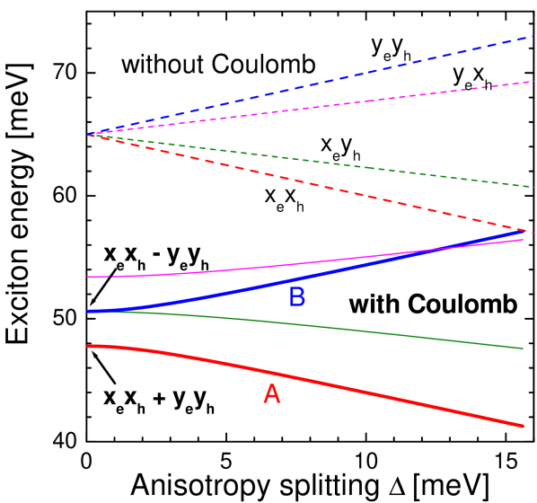
Figure 1. Energies of exciton excited states in anisotropic pancake InGaAs QDs calculated with (full curves) and without (dashed curves) Coulomb interaction. A and B are the two bright excited states (thick lines).

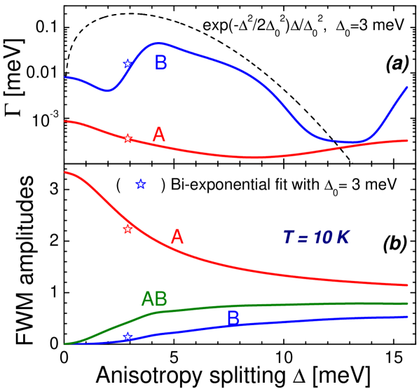
Figure 2. Dephasing rates (a) and FWM amplitudes (b) of the bright excited states at $T=10$ K. Bi-exponential fit of the ensemble-averaged photon echo is shown by stars. The splitting distribution function is shown by a dashed line.

4. Dephasing of QD excited states

In order to simulate the measurable time-integrated FWM, we consider an ensemble of QDs of different size and shape. Variations of the QD size are mainly responsible for a wide distribution ($\sim 30$ meV in InGaAs QDs [1]) of the exciton transition frequency. Due to the phase prefactor in Eq. (6), the transition frequency distribution leads to the photon echo effect: The FWM polarization from different dots destructively interfere at all times except those around $t=\tau$, and the measured signal is $P_{\rm echo}(\tau)=P_{\rm FWM}(\tau,\tau)$. In a proper simulation, the latter has to be additionally averaged over a distribution of the QD excited states splitting, which is much narrower ($\sim 3$ meV [1]) and is mainly due to QD shape variations.

To do this, we assume a pancake shape of a QD (having a smaller size in $z$-direction) with parabolic potentials for electrons and holes, which are additionally anisotropic in the $xy$-plane. Here we concentrate on exciton excited states formed from $x$- and $y$-type electron and hole states. Without Coulomb interaction the electron-hole pair has two bright ($x_{e}x_{h}$ and $y_{e}y_{h}$) and two dark states ($x_{e}y_{h}$ and $y_{e}x_{h}$). Their energies are shown in Fig. 1 (dashed curves) as functions of the anisotropy splitting $\Delta\equiv E_{y_{e}y_{h}}\!-\!E_{x_{e}x_{h}}$. Switching on the Coulomb interaction adds to the exciton Hamiltonian a block-diagonal matrix, the bright and the dark states not talking to each other (due to parity), and brings in an additional energy splitting within each doublet (Fig. 1, solid curves). At $\Delta=0$ bright exciton states $A$ and $B$ are, respectively, exact symmetric and antisymmetric combinations of the former states, the lower state $A$ accumulating the whole oscillator strength [see Fig. 2 (b)].

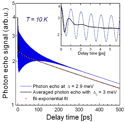
Figure 3. Photon echo signal of anisotropic QD calculated for $\Delta=2.9$ meV (thin curve) and the ensemble-averaged photon echo (thick curve), at long times fitted by two exponents (circles). Inset: the same in the short-time scale.

Quite explicitly, for these excited states the photon echo can be now written as

$$P_{\rm echo}(\tau)=\mu_{A}^{4}\,C_{A}(\tau)\,e^{-2\Gamma_{A}\tau}+\mu_{B}^{4}\,C_{B}(\tau)\,e^{-2\Gamma_{B}\tau}+2\mu_{A}^{2}\mu_{B}^{2}\,C_{AB}(\tau)\,e^{-(\Gamma_{A}+\Gamma_{B})\tau}\,\cos(\omega_{A}-\omega_{B})\tau.$$ (9)

Remarkably, the dephasing rates $\Gamma_{A}$ and $\Gamma_{B}$ which show up in the FWM polarization, Eq. (9), turn out to be exactly the same as in the linear polarization. The lower state ($A$) which is considerably split off has a rather weak dephasing at $T=10$ K [Fig. 2 (a)] which is mainly due to virtual transitions. The upper state, in turn, is always close to one of the dark states and has a much stronger dephasing due to real transitions. It rapidly changes with $\Delta$ having maxima when the level distance is close to the typical energy ($\sim 2$ meV) of the acoustic phonons coupled to the QD. The photon echo amplitudes shown in Fig. 2 (b) are mainly determined by the exciton dipole moments $\mu_{A}$, $\mu_{B}$. The functions $C_{i}(\tau)$ in Eq. (9) change rapidly at short times, while becoming constants in the long-time limit. These constant final values are nothing else than the zero-phonon weights which at low temperatures do not differ too much from unity.

The photon echo signal, Eq. (9), shown in Fig. 3 for $\Delta=2.9$ meV (thin curves) have oscillations up to 200 ps due to the mixed $AB$-term. The rapid short-time decay (corresponding to the broadband in the spectrum) is also seen as lowering of both maxima and minima (see the inset in Fig. 3). We finally perform the averaging over an ensemble of QDs having different $xy$-anisotropy degree: $\bar{P}_{\rm echo}(\tau)=\int_{0}^{\infty}\!d\Delta\,P_{\rm echo}(\tau;\Delta)\,e^{-\Delta^{2}/2\Delta_{0}^{2}}\,\Delta/\Delta_{0}^{2}$, where $\Delta_{0}=3$ meV is used. The averaged function $\bar{P}_{\rm echo}(\tau)$ has oscillations only in the time scale of $2\pi\hbar/\Delta_{0}$ (Fig. 3, thick curves). At later times it is well approximated by a sum of two exponents (Fig. 3, circles) with decay times 20.8 ps and 922 ps. The amplitudes and half decay rates of the bi-exponential fit are marked in Fig. 2 by stars. Both amplitudes and rates are very close to those of the photon echo signal ${P}_{\rm echo}(\tau)$ of the particular QD with $\Delta=2.9$ meV. Thus, we believe that the measured double-exponential long-time decay [1] is due to the two bright excited states in QD, which have quite different dephasing times at low temperatures.

We thank P. Borri and W. Langbein for stimulating discussions. Financial support by DFG Sonderforschungsbereich 296 is gratefully acknowledged. E. A. M. acknowledges partial support by Russian Foundation for Basic Research and Russian Academy of Sciences.

References

- [1] P. Borri and W. Langbein, 9th Conference on Optics and Excitons in Confined Systems, Abstracts, Southampton (2005), p. 50.
- [2] P. Borri, W. Langbein, S. Schneider, U. Woggon, R. L. Sellin, D. Ouyang, and D. Bimberg, Phys. Rev. Lett. 87, 157401 (2001).
- [3] P. Borri, W. Langbein, U. Woggon, V. Stavarache, D. Reuter, and A. D. Wieck, Phys. Rev. B 71, 115328 (2005).
- [4] P. Borri, W. Langbein, U. Woggon, M. Schwab, M. Bayer, S. Fafard, Z. Wasilewski, and P. Hawrylak, Phys. Rev. Lett. 91, 267401 (2003).
- [5] A. Vagov, V. M. Axt, and T. Kuhn, Phys. Rev. B 66, 165312 (2002).
- [6] A. Vagov, V. M. Axt, and T. Kuhn, Phys. Rev. B 67, 115338 (2003).
- [7] G. Mahan, Many-Particle Physics, (Plenum, New York, 1990).
- [8] A. Vagov, V. M. Axt, and T. Kuhn, W. Langbein, P. Borri, and U. Woggon, Phys. Rev. B 70, 201305 (2004).
- [9] E. A. Muljarov and R. Zimmermann, Phys. Rev. Lett. 93, 237401 (2004).
- [10] E. A. Muljarov, T. Takagahara, and R. Zimmermann, Phys. Rev. Lett. 95, 177405 (2005).