Anomalous dynamics in two– and three– dimensional Heisenberg-Mattis spin glasses

Abstract

We investigate the spectral and localization properties of unmagnetized Heisenberg-Mattis spin glasses, in space dimensionalities $d=2$ and $3$, at $T=0$. We use numerical transfer-matrix methods combined with finite-size scaling to calculate Lyapunov exponents, and eigenvalue-counting theorems, coupled with Gaussian elimination algorithms, to evaluate densities of states. In $d=2$ we find that all states are localized, with the localization length diverging as $\omega^{-1}$, as energy $\omega\to 0$. Logarithmic corrections to density of states behave in accordance with theoretical predictions. In $d=3$ the density-of-states dependence on energy is the same as for spin waves in pure antiferromagnets, again in agreement with theoretical predictions, though the corresponding amplitudes differ.

I Introduction

The study of low-lying magnetic excitations in quenched disordered systems presents a number of challenges. While the absence of translational invariance is a complicator arising in all aspects both of static and dynamic behavior of inhomogeneous magnets, investigation of spin waves is made even harder because, in many cases of interest, the exact ground state configuration is not known.

One way around the latter obstacle has been to resort to simplified model systems for which the exact ground state is known, but which nevertheless still display non-trivial dynamical features. Such features, it is expected, may shed light on the behavior of their experimentally-realized, rather more complex, counterparts.

Here we deal with vector spin glasses, i. e., Heisenberg spins with competing ferro– and antiferromagnetic interactions. It is known that the simplest realization of the Edwards-Anderson picture, where one has equal concentrations of positive and negative nearest-neighbor bonds of equal strength, leads (in lattices of space dimensionality $d>1$) to frustration and, consequently, to a macroscopically degenerate (classical) ground state.

The drawback just described does not arise in Mattis spin-glasses, where the Mattis transformation dcm76 “gauges away” disorder effects, as far as most static aspects are concerned. It is known that the Mattis transformation does not remove the disorder effects in the dynamics of these so-called Heisenberg-Mattis spin glasses, which is non-trivial. Indeed, investigations of spin-wave propagation in such systems ds77 ; clh77 ; ds79 ; ch79 ; sp88 ; ga04 have unveiled many features which stand in stark contrast, e.g., to the Halperin-Saslow (hydrodynamic) picture hs77 of a linear dispersion relation for low-energy excitations.

Here, we shall assume that the spin magnitude is $|{\mathbf{S}}|\gg 1$, so that quantum fluctuations can be safely neglected sp88 ; ga04 (classical limit).

An alternative to using the Mattis picture can be pursued by studying usual spin glasses (i.e. with random $\pm J$ bonds) in the high-field limit, as this additional feature stabilizes a ferromagnetic-like ground state while still incorporating quenched (bond) disorder ahc92 ; ah93 ; ahc93 . However, results thus obtained differ rather drastically from those pertaining to the zero-field case. In fact, it has been found that, even in zero field and space dimensionality $d=1$ where frustration effects are absent, “unmagnetized” spin glasses (i.e. in which the concentrations of ferro- ($p$) and antiferromagnetic ($1-p$) bonds are equal) differ substantially from their “magnetized” ($p\neq 1/2$) counterparts ew92 .

In this paper, we investigate the spectral and localization properties of Heisenberg-Mattis spin glasses. Our emphasis is on unmagnetized systems in space dimensionalities $d=2$ and $3$, at $T=0$. We use numerical transfer-matrix methods to calculate Lyapunov exponents ps81 ; bh89 ; ew92 , and eigenvalue-counting theorems, coupled with Gaussian elimination algorithms sb83 ; sne86 , to evaluate densities of states. Though early numerical studies clh77 ; ch79 already highlighted a number of distinctive features exhibited by such systems, motivation for further research is to be found in recent theoretical insights gc03 ; ga04 , especially in connection with the low-energy, long-wavelength regime.

In Section II we recall pertinent aspects of Heisenberg-Mattis spin glasses. Section III reports on an extension, to $d=2$ and $3$, of the analytical scaling techniques introduced in Ref. sp88, for $d=1$; in Section IV we report numerical calculations of Lyapunov exponents and of densities of states, for $d=2$ and $3$. Finally, in section V, concluding remarks are made.

II Heisenberg-Mattis spin glasses

We consider Heisenberg spins on sites of a square, or simple-cubic, lattice, with nearest-neighbor couplings:

$${\cal H}=-\sum_{\langle i,j\rangle}J_{ij}\,{\mathbf{S}}_{i}\cdot{\mathbf{S}}_{j}$$ (1)

The bonds are randomly taken from a quenched, binary probability distribution,

$$P(J_{ij})=p\,\delta(J_{ij}-J_{0})+(1-p)\,\delta(J_{ij}+J_{0})\ ,$$ (2)

so for $p=1/2$ one has the unmagnetized spin glass.

The Mattis model ascribes disorder to sites rather than bonds ($J_{ij}\to J_{0}\,\zeta_{i}\,\zeta_{j}$), so that the Hamiltonian reads:

$${\cal H}_{M}=-J_{0}\sum_{\langle i,j\rangle}\zeta_{i}\,\zeta_{j}\,{\mathbf{S}}_{i}\cdot{\mathbf{S}}_{j}\ ,$$ (3)

where $\zeta_{i}=+1$ ($-1$) with probability $p$ ($1-p$). This way, the overall energy is minimized by making $S_{i}^{z}=\zeta_{i}\,S$, which constitutes a (classical) ground state of the Hamiltonian Eq. (3), to be referred to as $|\,0\rangle$. Thus, disorder is effectively removed from static properties, but not from the dynamics, because of the handedness of Heisenberg spin commutation relations. Indeed, considering low-energy excitations, the equations of motion for the spins are, with $\hbar=1$:

$$i\,dS_{i}^{-}/dt=\sum_{j}J_{0}\,\zeta_{i}\,\zeta_{j}\,\left(S_{i}^{-}\,S_{j}^{z}-S_{j}^{-}\,S_{i}^{z}\right)\ ,$$ (4)

where $S_{i}^{\pm}=S_{i}^{x}\pm i\,S_{i}^{y}$ etc and $j$ are nearest neighbors of site $i$. So, putting $v_{i}\equiv\zeta_{i}\,S_{i}^{-}$, one gets sp88 , upon application of Eq. (4) to $|\,0\rangle$ :

$$i\,\zeta_{i}\,du_{i}/dt=\sum_{j}J_{0}\,\left(u_{i}-u_{j}\right)\ .$$ (5)

where the $u_{i}$ are Mattis-transformed local (on-site) spin-wave amplitudes. For the eigenmodes with frequency $\omega$ (in units of the exchange constant $J_{0}$), Eq. (5) leads to

$$\omega\,\zeta_{i}\,u_{i}=\sum_{j}\left(u_{i}-u_{j}\right)\ .$$ (6)

Goldstone modes are expected to occur, since disorder does not destroy the symmetry of the system in spin space gc03 . The relationship of frequency to wave number, $k$, at low energies is characterized by the dynamic exponent $z$:

$$\omega\propto k^{z}\ .$$ (7)

In $d=1$, where the scattering length coincides with the localization length ga04 , the definition of $k$ is unique. Indeed, numerical calculations bh89 ; ew92 ; ah93 of the $d=1$ density of states and of the Lyapunov exponent point to the same value $z=3/2$, predicted analytically sp88 . For $d>1$ this degeneracy is expected to be lifted. As we shall see below, different exponents come up, depending on whether localization or density-of-states properties are being considered.

III Scaling

We briefly review the treatment of one-dimensional systems, given in Ref. sp88, . In this case, Eq. (6) becomes

$$(2-\zeta_{i}\,\omega)\,u_{i}=u_{i-1}+u_{i+1}\ .$$ (8)

A transfer-matrix (TM) approachhori ; ps81 , can be formulated, giving sp88 ; bh89 ; ew92 :

$$\begin{pmatrix}{u_{i+1}}\cr{u_{i}}\end{pmatrix}=\begin{pmatrix}{2-\zeta_{i}\,\omega}&{-1}\cr{1}&{0}\end{pmatrix}\begin{pmatrix}{u_{i}}\cr{u_{i-1}}\end{pmatrix}=T_{i}(\omega)\,\begin{pmatrix}{u_{i}}\cr{u_{i-1}}\end{pmatrix}\ .$$ (9)

The allowed frequencies for a chain with $N$ spins and periodic boundary conditions, $u_{N+1}\equiv u_{1}$, are determined by ${\rm det}\,(\Lambda_{N}-1)=0$, where

$$\Lambda_{N}(\omega)=\prod_{i=1}^{N}T_{i}(\omega)\ ;$$ (10)

equivalently, the condition ${\rm Tr}\,\Lambda_{N}=2$ determines the eigenfrequencies. Scaling the system by a linear dilation factor $b$, the dynamics is preserved if the frequencies are transformed ($\omega\to\omega^{\prime}$), in such a way that

$${\rm Tr}\,\Lambda_{N}(\omega)={\rm Tr}\,\Lambda_{N/b}(\omega^{\prime})\ .$$ (11)

Using properties of the matrices $T_{i}(\omega)$, one finds sp88 that the first-order term (in $\omega$) of ${\rm Tr}\,\Lambda_{N}(\omega)$ has a coefficient equal to $N\sum_{i=1}^{N}\zeta_{i}$. Therefore, correspondence of the $\{\zeta_{i}\}$ with an unbiased random-walk makes the determining variable $\omega\,N^{3/2}$, so that the (length) scaling of the frequencies is $\omega^{\prime}=\omega\,b^{3/2}$, and the low-energy dispersion relation Eq. (7) has an anomalous power (dynamic exponent) $z=3/2$. In fact, careful consideration of higher-order terms sp88 shows that the combination $N^{3/2}\,\omega$ is present to all orders, thus scaling is expected to hold even away from the $\omega\to 0$ region (though not the single power-law form, Eq. (7)).

A suitable framework for extensions of this treatment to space dimensionalities $d>1$ is found in quasi– one dimensional geometries, i.e. $L^{d-1}\times N$ systems with $N\gg 1$. In what follows, we shall always make use of periodic boundary conditions across the $d-1$ transverse directions.

Considering $d=2$ for simplicity, a TM can be set up on a strip of width $L$ sites, so an $L$- component vector ${\vec{u}}_{i}=(u_{1i},\cdots,u_{Li})$ corresponds to each column $i$ along the strip, with the recursion relation

$$\begin{pmatrix}{{\vec{u}}_{i+1}}\cr{{\vec{u}}_{i}}\end{pmatrix}=T_{i}^{2d}(\omega)\,\begin{pmatrix}{{\vec{u}}_{i}}\cr{{\vec{u}}_{i-1}}\end{pmatrix}\ ,$$ (12)

where

$$T_{i}^{2d}(\omega)=\begin{pmatrix}{M_{i}}&{-I}\cr{I}&{0}\end{pmatrix}\,\quad M_{i}=a-\omega b_{i}\ ,$$ (13)

$I$ being the $L\times L$ identity matrix, while $a$ and $b_{i}$ are given by:

$${a}=\begin{pmatrix}{4}&{-1}&{\ \,0}&{\cdots}&{-1}\cr{-1}&{4}&{-1}&{\cdots}&{\ 0}\cr{\cdots}&{\cdots}&{}&{}&{-1}\cr{-1}&{\ 0}&{\cdots}&{-1}&{\ 4}\end{pmatrix}\,;\,b_{i}=\begin{pmatrix}{\zeta_{1i}}&{\ \,0}&{\cdots}&{0}\cr{0}&{\zeta_{2i}}&{0}&{\cdots}\cr{\cdots}&{\cdots}&{}&{0}\cr{\ 0}&{\cdots}&{0}&{\ \zeta_{Li}}\end{pmatrix}\,.$$ (14)

Hence,

$$T_{i}^{2d}(\omega)=\begin{pmatrix}{a}&{-I}\cr{I}&{0}\end{pmatrix}-\omega\begin{pmatrix}{b_{i}}&{0}\cr{0}&{0}\end{pmatrix}\equiv A-\omega\,B_{i}\ .$$ (15)

Generalizations to higher $d$ are immediate, with the vector ${\vec{u}}_{i}$ now having $L^{d-1}$ components, and the matrices $I$, $a$ and $b_{i}$ being $L^{d-1}\times L^{d-1}$. The $(2L^{d-1}\times 2L^{d-1})$ matrix $T_{i}$ is symplectic, that is, its eigenvalues occur in pairs $\{\nu_{i},\nu_{i}^{-1}\},\ i=1,\dots,L^{d-1}$. Note that matrix $A$ is symplectic as well.

For $d>1$, a feature which does not occur in the one-dimensional case is that there are transverse momentum modes. Returning to $d=2$ for illustration, these are indeed the eigenmodes of matrix $a$ in Eq. (14), with corresponding energies $\varepsilon_{p}=4-2\cos 2\pi p/L$, $p=0,1,\dots,L-1$.

We briefly make contact with the analogous case of a homogeneous system of length $N$, for which $b=I$, $[a,b]=0$, and the eigenstates of $a$ are also eigenstates of the full hamiltonian, with $\omega_{pq}=\varepsilon_{p}-2\cos 2\pi q/N$, $q=0,1,\dots,N-1$. This reminds us that, in $d>1$, the energy of a mode is not related only to its longitudinal wavevector, as is the case in $d=1$. Upon introduction of randomness, the commutation relation is destroyed (contrary to the one-dimensional case where both $a$ and $b$ are numbers) and, consequently, the interplay between frequency- and wavevector- aspects can only be measured via the accumulated statistics of many local realizations of disorder. Therefore, in $d>1$ one may expect the picture of a single length controlling both (spatial) attenuation and (time) oscillation damping sp88 , which holds for $d=1$ spin glasses, to be replaced by one where each of these properties is governed by a distinct quantity.

We now return to spin glasses. From the eigenvectors of $a$, “spinor” generalizations can be built, which are eigenvectors of $A$, with eigenvalues $(\nu_{p},\nu_{p}^{-1})$ indexed by $p$; one can show that $\nu_{p}+\nu_{p}^{-1}=\varepsilon_{p}$. While such spinors are obviously not eigenvectors of $B$, the contribution given by each diagonal element of $T_{i}^{2d}(\omega)$, corresponding to fixed $p$, to the trace of $\Lambda_{N}^{2d}(\omega)\equiv\prod_{i=1}^{N}T_{i}^{2d}(\omega)$, can be worked out to first order in $\omega$. Use is made of the fact that, analogously to the $d=1$ case sp88 ,

$$\prod_{\ell=1}^{N}T_{\ell}^{2d}(\omega)=A^{N}-\omega\,\sum_{\ell=1}^{N}A^{\ell-1}\,B_{\ell}\,A^{N-\ell}+{\cal O}(\omega^{2})\ .$$ (16)

The result is:

$${\rm Tr}\,(p)\prod_{\ell=1}^{N}T_{\ell}^{2d}(\omega)=\nu_{p}^{N}+\nu_{p}^{-N}-$$

$$-\omega\,\frac{(\nu_{p}^{N}-\nu_{p}^{-N})}{\nu_{p}-\nu_{p}^{-1}}\sum_{\ell=1}^{N}\sum_{m=1}^{L}\frac{1}{L}\,\zeta_{m\ell}+{\cal O}(\omega^{2})\ ,$$ (17)

where ${\rm Tr}\,(p)$ denotes the joint contribution of both eigenspinors of $A$ indexed by $p$ (associated respectively to eigenvalues $\nu_{p}$ and $\nu_{p}^{-1}$).

The “critical” (large scale) behavior is associated with small $p$, in which case $\nu_{p},\ \nu_{p}^{-1}\to 1$, and Eq. (17) turns into:

$${\rm Tr}\,(p)\prod_{\ell=1}^{N}T_{\ell}^{2d}(\omega)\to 2-\omega\,N\sum_{\ell=1}^{N}\frac{1}{L}\,\sum_{m=1}^{L}\zeta_{m\ell}+{\cal O}(\omega^{2})\ .$$ (18)

One can readily see that, for generic $d>1$, this translates into:

$${\rm Tr}\,(p)\prod_{\ell=1}^{N}T_{\ell}(\omega)\to 2-$$

$$-\omega\,N\sum_{\ell=1}^{N}\left(\prod_{i=1}^{d-1}\frac{1}{L_{i}}\,\sum_{m_{i}=1}^{L_{i}}\,\zeta_{m_{1}\cdots m_{d-1}\ell}\right)+{\cal O}(\omega^{2})\ .$$ (19)

In the second term of Eq. (19), one has a sum of $N\times L_{1}\times\cdots\times L_{d-1}$ binary random variables, so this is gaussian distributed with rms value:

$$\frac{\omega\,N}{\prod_{i=1}^{d-1}L_{i}}\,\left(N\prod_{i=1}^{d-1}L_{i}\right)^{1/2}=\frac{\omega\,N^{3/2}}{\left(\prod_{i=1}^{d-1}L_{i}\right)^{1/2}}\ .$$ (20)

Upon scaling of linear dimensions by a factor $b$, under which frequency scales as $\omega\to b^{z}\,\omega$, and requiring invariance of the term given in Eq. (20) (see Eq. (11)), one gets:

$$z=2-\frac{d}{2}=\begin{cases}\frac{3}{2}&d=1\cr 1&d=2\cr\frac{1}{2}&d=3\cr\end{cases}\ .$$ (21)

Consideration of the terms in Eq. (18) of higher than first order in $\omega$ shows that, unlike the $d=1$ case, the trace of the full TM is not just a function of the variable given in Eq. (20), because complicated sums occur, involving both longitudinal and transverse wave vectors.

This is in line with the reasoning presented above, to the effect that the simultaneous presence of both longitudinal and transverse degrees of freedom invalidates the single-length picture, predicted analytically sp88 and numerically confirmed ah93 ; bh89 ; ew92 for $d=1$.

While it is plausible to expect that, for some low-energy regime in $d>1$ the scaling result, Eq. (21) might hold true, direct verification is called for.

IV Numerical analysis

IV.1 Lyapunov exponents

The procedure for calculating Lyapunov exponents on strips or bars is the same as that used for Anderson localization problems ps81 . Indeed, in both cases the TM is symplectic, and one can use Oseledec’s theorem and dynamic filtration to extract the smallest Lyapunov exponent, whose inverse is the largest localization length. For Heisenberg spin-glass chains, this has been done ew92 ; bh89 , numerically confirming the result $z=3/2$ obtained analytically in Ref. sp88, .

We have investigated strips of widths $L=4,6,\cdots,14$ in $d=2$, in which for each energy $\omega$ we took $N=10^{6}$ iterations of the TM, and bars with $L\times L$ cross-section, $L=4,6,8,10$ in $d=3$. In $d=3$ we used $N=10^{6}$ for $L=4,6$, $5\times 10^{5}$ for $L=8$, and $1\times 10^{5}$ for $L=10$.

In contrast with $d=1$, here one must take into account finite-size effects, introduced via the transverse dimension $L$, thus calculated localization lengths are denoted by $\lambda_{L}$. Using standard finite-size scaling theory fs2 , it is expected that the behavior of scaled localization lengths $\lambda_{L}/L$, when plotted against $\omega\,L^{z}$, will allow one to infer the bulk ($L\to\infty$) properties of the system.

Figure 1: Scaling plot for localization lengths on strips of a $d=2$ system, against $\omega\,L^{z}$, with $z=1$ as predicted in Eq. (21). Strip widths $L$ as given by symbols. Line corresponds to $y\propto x^{-2/3}$ and is a guide to the eye, showing how the effective $d=1$ regime sets in for very low energies. Insert: unscaled data for $L=4$ and $14$.

In Fig. 1 we see that in $d=2$ good data collapse, extending as far as $x\equiv\omega\,L^{z}\simeq 0.3$, is achieved when $z=1$, as predicted in Eq. (21). At the low-energy end, $x\lesssim 0.03$, the quasi-one dimensional character of the strips begins to dominate, and the scaling curve crosses over to the effective $d=1$ regime characterized by $\omega\sim k^{3/2}$.

Figure 2: Scaling plot for localization lengths on bars of a $d=3$ system, against $\omega\,L^{z}$, with $z=1/2$ as predicted in Eq. (21). Bar cross-sections are $L\times L$, with $L$ as given by symbols. Line corresponds to $y\propto x^{-2/3}$ and is a guide to the eye, showing how the effective $d=1$ regime sets in for very low energies. Insert: unscaled data for $L=4$ and $10$.

In Fig. 2 the scaling plot for $d=3$, with $z=1/2$ as predicted in Eq. (21), is exhibited. The quality of data collapse is remarkably inferior to that of $d=2$ data. An examination of the behavior of $\lambda_{L}/L$ against $\omega$ shows that curves corresponding to pairs $L,L-2$ have well-defined crossings at low energies $\omega\lesssim 0.05$. The usual interpretation of these, in the finite-size scaling context, would point to a localization-delocalization transition ps81 ; fs2 . However, we have found that the locations of crossings appear to approach $\omega=0$ with increasing $L$. This would be consistent with the idea that all magnons are delocalized in $d=3$, which is supported, e.g., by the field-theoretical results of Ref. ga04, . We postpone a discussion of this point (and similar ones associated to the behavior found above for $d=2$), to Section V.

IV.2 Densities of states

The calculation of densities of states per unit energy interval (DOS), ${\cal D}(\omega)$, and their integrated counterparts (IDOS), $N(\omega)=\int_{-\infty}^{\omega}{\cal D}(\omega^{\prime})\,d\omega^{\prime}$, makes use of eigenvalue-counting theorems dean ; dm60 ; tho72 . Our implementation resorts to Gaussian elimination algorithms on quasi one-dimensional geometries ($L^{d-1}\times N$, with $N\gg L$), and closely follows the steps described in Refs. sb83, ; sne86, where the systems under investigation were, respectively, phonons in disordered solids, and tight-binding electrons (Anderson localization). The key feature shared between these problems and the one studied here is the fact that, for an $L^{d-1}\times N$ system with periodic boundary conditions across, the hamiltonian has a $(2\times L^{d-1}+1)$- diagonal form, i.e., it can only have non-zero elements in the $L^{d-1}$ lines above, and $L^{d-1}$ lines below, the diagonal.

We consider the characteristic matrix, which in the present case is $C=\zeta\omega\,I-{\cal H}$, where $\zeta\omega\,I$ is a diagonal matrix with $[\zeta\omega\,I]_{jj}=\zeta_{j}\,\omega$ ($j=$ site index), for an $L^{d-1}\times N$ system. Evaluation of its diagonal elements via Gaussian elimination enables one to obtain the IDOS for any energy sb83 ; sne86 , thus the DOS may be calculated by numerical differentiation.

For $d=1$ the eigenvalue counting (used., e.g., in Ref. ew92, ), may, alternatively, proceed via enumeration of nodes of the amplitude ratios which enter the evaluation of the (single) Lyapunov exponent bh89 ; ah93 . In order to test our recursion and elimination algorithms, we applied them to this case and compared the outcome with that from node-enumeration . Results are identical to within numerical accuracy, and the set produced by Gaussian elimination is depicted in Fig. 3.

Figure 3: Double-logarithmic plot of density of states ${\cal D}(\omega)$ for spin-glass chain, calculated by Gaussian elimination. Chain length $N=10^{7}$ sites. Thick line is the exact Derrida-Gardner result dg84 (with coefficient doubled, on account of different normalization, see text).

By sampling energies separated by logarithmically uniform intervals, we achieved a detailed view of the $\omega\to 0$ region, which is difficult to isolate in the corresponding DOS results of Refs. bh89, ; ew92, ; ah93, (where linear binning was used). One sees that the relationship ${\cal D}(\omega)\propto\omega^{-1/3}$ is valid for more than two orders of magnitude in energy, up to $\omega\simeq 0.3$. For guidance, we have also included the exact Derrida-Gardner result dg84 . Since we have considered only positive energy states in our calculation, the appropriate proportionality coefficient is twice that given in Ref. dg84, .

For higher-dimensional cases, is is worth mentioning that the algorithms used here are much less computationally intensive than their Lyapunov-exponent counterparts. For an $L^{d-1}\times N$ system, the computational time rises as $L^{3(d-1)}\times N$ for the former sne86 , and approximately as $L^{5(d-1)}\times N$ for the latter. This is mainly because of the frequent mutual orthogonalization of $2\times L^{d-1}$ iterated vectors, which is necessary in order to avoid cross-contamination between eigenvectors associated to different Lyapunov exponents. Therefore, for DOS and IDOS it is usually possible (except for very low energies in $d=3$, see below) to work with systems whose transverse dimensions $L$ are large enough that finite-size effects are of little import. It remains only to make sure that the sample length $N$ is long enough, in order to achieve adequate sampling of quenched disorder configurations.

We examined the effect of finite transverse dimensions, by evaluating pure-system quantities and comparing our results to the exact ones. Though, having zero net magnetization, the spin glasses studied here are closer to antiferromagnets (AF) than to homogeneous ferromagnets (FM), the DOS and IDOS of magnons in the latter exhibit some distinctive features, whose numerical reproduction is a non-trivial test of the adequacy and accuracy of our methods. For FM in $d=2$, already with $L=25$, $N=2500$ the IDOS is at most $3\%$ off the exact value. This largest discrepancy happens close to $\omega=4$ where the analytical IDOS exhibits an inflection point, on account of the DOS’s logarithmic Van Hove singularity at the band center. Increasing $L$ or $N$ does not significantly reduce the deviation close to $\omega=4$; however, it does improve agreement elsewhere on the energy axis. The calculated DOS is rather sensitive to discrete-lattice effects; nevertheless, the consequent oscillations are again much diminished by increasing $L$, $N$. For $d=3$ FM, the relatively featureless IDOS is easier to reproduce. With $L=16$, $N=25600$, deviations are down to, at most, $1.5\%$ (though the DOS still displays somewhat large oscillations, especially around the “knees” at $\omega=4$ and $8$).

Figure 4: DOS (${\cal D}(\omega)$) and IDOS ($N(\omega)$) for pure FM systems against normalized energy $\omega/\omega_{0}$: analytical (lines) and calculated by Gaussian elimination (points). Dashed lines and triangles: ${\cal D}(\omega)$; full lines and squares: $N(\omega)$. (a): $d=2$, $L=100$, $N=50000$. (b): $d=3$, $L=16$, $N=25600$. The pure-system (FM) bandwidth is $\omega_{0}^{F}=8$ $(d=2)$, and $12$ $(d=3)$.

Fig. 4 shows representative results, which are useful as guidelines for the investigation of disordered systems in $d=2$ and $3$ via Gaussian elimination.

Turning to pure AF systems, for which the respective bandwidths are $\omega_{0}^{AF}=4$ $(d=2)$, and $6$ $(d=3)$, again relatively small transverse dimensions $L$ provide results which closely follow the analytic values, except at very low $\omega$. In this limit, the fact that the finite $L$ quantizes the transverse momentum leads to effective one-dimensional behavior (${\cal D}(\omega)\sim\omega^{0}$, $N(\omega)\sim\omega^{1}$) for $\omega$ less than a crossover frequency $\omega_{m}\equiv A_{\,\rm AF}(d)/L^{z}$, $z=1$. With the units used in this work, we found $A_{\,\rm AF}(2)\simeq 12$, $A_{\,\rm AF}(3)\simeq 20$. The effect is more pronounced here than for FM, where $z=2$ and, consequently, the onset of this sort of behavior occurs at much lower energies. Fig. 5 highlights the worst case of $d=3$. For completeness, the inset of Fig. 5 shows that, even for $L=16$ where these low-energy discrepancies are rather severe, agreement with analytical forms is quite satisfactory elsewhere.

Figure 5: Low-energy IDOS, $N(\omega)$, for pure AF in $d=3$ against energy $\omega$: analytical (full line) and calculated by Gaussian elimination on $L^{2}\times N$ systems, $N=500\,L^{2}$ (points, connected by dashed lines). Triangles: $L=16$; squares: $L=20$; circles: $L=24$. Inset: full-band IDOS (same axes as main Figure). Analytical (full line), and Gaussian elimination with $L=16$ (triangles).

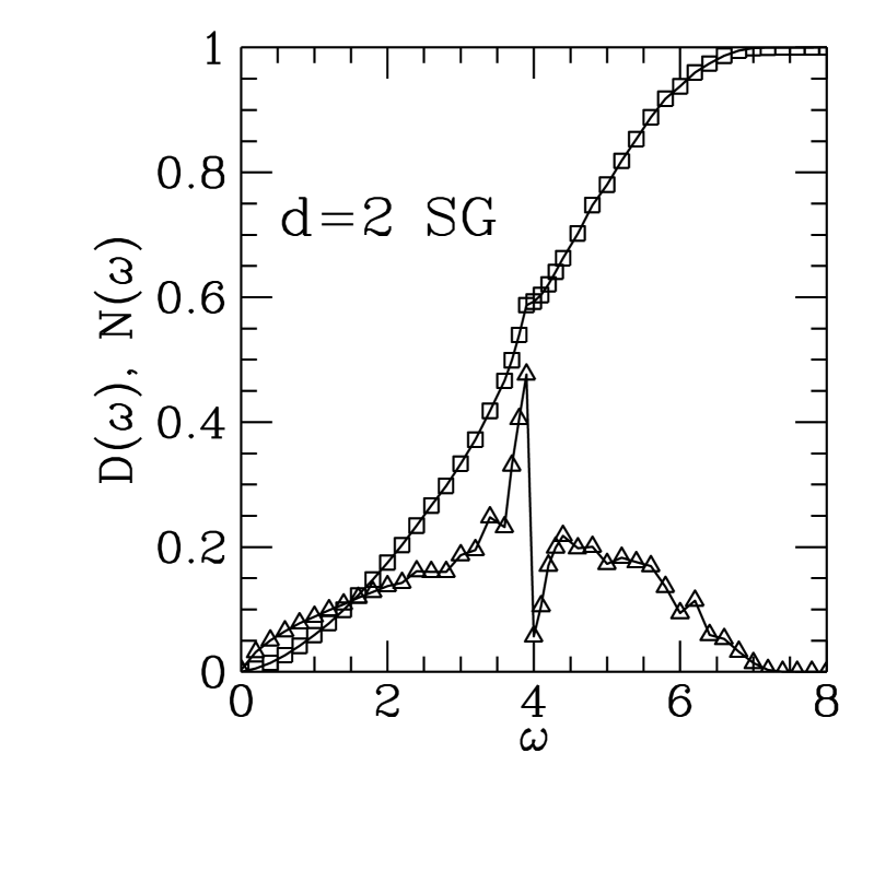
Figure 6: DOS (${\cal D}(\omega)$) and IDOS ($N(\omega)$) for Mattis spin glass in $d=2$, against energy $\omega$, calculated by Gaussian elimination. Triangles: ${\cal D}(\omega)$; squares: $N(\omega)$. $L=250$, $N=2.5\times 10^{6}$.

We now return to disordered systems. In Fig. 6, results for the Mattis spin glass in $d=2$ are presented. We used $L=250$, $N=2.5\times 10^{6}$. The number of sites entering the calculation was more than one order of magnitude larger than in that for a pure FM, whose result is exhibited in Fig. 4 (a). From examination of shorter runs for the disordered case, it appears that the features displayed in Fig. 6 are rather stable and well-converged. For this value of $L$, the crossover to one-dimensional behavior, referred to above, is confined to $\omega\lesssim 0.05$, leaving a broad window at low energies for which genuine two-dimensional behavior can be observed. The main distinctions of the IDOS from its pure-system (FM and AF) counterparts are: (i) close to $\omega=4$, the upper limit of the AF band, the FM IDOS’s inflection point is replaced by a seeming “knee”, with a short flat section; and (ii) saturation is reached below the FM band edge $\omega_{0}^{F}=8$, but above the AF edge $\omega_{0}^{AF}=4$; by $\omega=6.7$ the IDOS is already within less than $1\%$ of unity. Similar effects can be seen in early numerical work ch79 , though in that Reference saturation appears to be reached only above the FM band edge, at $\omega\simeq 9.0$.

It has been predicted ds79 ; ga04 that, since $d=2$ is the critical dimensionality in this case gc03 , the two-dimensional spin glass will behave as a pure (AF) system (namely, ${\cal D}(\omega)\sim\omega^{1}$, $N(\omega)\sim\omega^{2}$), with logarithmic corrections. At low frequencies, the real part of the dispersion relation is expected to follow the expression ds79 ; ga04 :

$${\rm Re}\ \omega\propto\frac{p}{\sqrt{\log\left(\frac{\Lambda}{p}\right)}}\ ,$$ (22)

where $\Lambda$ is a momentum cutoff, reciprocal to the minimum wavelength of magnons. From Eq. (22), one can work out the predicted behavior of the IDOS at low energies. This turns out to be:

$$N(\omega)\propto\omega^{2}\,\ln\left(\frac{\Omega}{\omega}\right)\ ,$$ (23)

where $\Omega$ is a cutoff frequency, corresponding to the momentum cutoff $\Lambda$.

We have tested the prediction, Eq. (23), against our data, with the results shown in Fig. 7. A fit of the raw data (crosses in Fig. 7) to pure power-law behavior gives $N(\omega)\sim\omega^{x}$, with the effective exponent $x\simeq 1.62$. On the other hand, plotting $N(\omega)/\ln(\Omega/\omega)$ against $\omega^{2}$ (squares in Fig. 7) removes just about all the curvature, provided that a suitable value of $\Omega$ is used. A linear least-squares fit of data for $0.05\leq\omega\leq 0.5$ (shown as a full line in Fig. 7) gives $\Omega=5.8(1)$, broadly consistent with the effective bandwidth $\gtrsim 6.7$ found above . Keeping $\Omega=5.8$, and fitting $N(\omega)/\ln(\Omega/\omega)$ to a power law dependence over the full interval $0.05\leq\omega\leq 1.0$, would give an effective power $x\simeq 1.04$.

Figure 7: IDOS ($N(\omega)$) for Mattis spin glass in $d=2$, for low energies, against $\omega^{2}$, calculated by Gaussian elimination. $L=250$, $N=2.5\times 10^{6}$. Crosses: $N(\omega)$; squares: $N(\omega)/\ln(\Omega/\omega)$, with $\Omega=5.8$ [see Eq. (23), and text]. Full line is a linear least-squares fit to data for $0.05\leq\omega\leq 0.5$.

We undertook similar calculations for the Mattis spin glass in $d=3$. Since one is above the critical dimensionality in this case ds79 ; gc03 , the three-dimensional spin glass is expected to behave as a pure (AF) system, at least at low energies and long wavelengths (namely, ${\cal D}(\omega)\sim\omega^{2}$, $N(\omega)\sim\omega^{3}$).

Similarly to the pure $d=3$ AF, for the ranges of $L$ within relatively easy reach of our calculations, the low-frequency spectrum exhibits a crossover towards one-dimensional behavior. With the terminology introduced above, this happens for $\omega\lesssim\omega_{m}$, $\omega_{m}=A_{\,\rm SG}(d)/L$; by examining the sequence $L=16,\,24,\,30,\,36$, we estimate $A_{\,\rm SG}(3)\simeq 11$, just over half the corresponding value for pure AF. Thus, such effects are once more confined to low energies. We have found that, for $\omega\gtrsim 1.2$, the $L=16$ curve is within less than $3\%$ of those corresponding to larger $L$, which are grouped together even more tightly. Fig. 8 presents an overall picture of results, for $L=16$, $N=2.56\times 10^{6}$. Again, early saturation occurs. The IDOS is within $0.1\%$ of unity by $\omega=9.4$, just over three-quarters of the FM band width $\omega_{0}=12$. A kink, similar to the one occurring in $d=2$ but less intense, arises close to the center of the FM band (and top of the AF one), $\omega=6$. Both features show up in Ref. clh77, , though with saturation occurring at a slightly higher energy (but still within the FM band).

Figure 8: DOS (${\cal D}(\omega)$) and IDOS ($N(\omega)$) for Mattis spin glass in $d=3$, against energy $\omega$, calculated by Gaussian elimination. Triangles: ${\cal D}(\omega)$; squares: $N(\omega)$. $L=16$, $N=2.56\times 10^{6}$.

The low-energy behavior is shown in Fig. 9. For $L=36$ we have found that least-squares fits of our calculated data (excluding the very low-energy intervals where one-dimensional behavior takes over) give $z=2.97(5)$, if we keep to $\omega\leq 1.0$; including higher energies (e.g. $\omega\lesssim 2.5-3.0$) results in a slight decrease of effective exponents, down to $z\simeq 2.75$. On the other hand, fits of the numerically-evaluated analytic IDOS for a cube with $100^{3}$ sites (shown in Fig. 9), when restricted to $\omega\leq 1.5$, give an effective $z=2.82(1)$; it is only when the upper limit is raised to $\omega=3.0$ that one reaches $z=2.99(1)$. This is because, in the low-energy limit, discrete-lattice effects still persist, which induce slight deviations of effective behavior away from the exact value $z=3$. In summary, it is only in the very low-energy limit $\omega\leq 1.0$ that the $d=3$ SG $N(\omega$) indeed exhibits the $\omega^{3}$ dependence characteristic of the pure AF.

Figure 9: Double-logarithmic plot of IDOS ($N(\omega)$) for Mattis spin glass in $d=3$, for low energies, against energy $\omega$, calculated by Gaussian elimination. Squares: calculated points, $L=36$, $N=6.48\times 10^{5}$. The straight line is a power-law fit with slope $2.97$ (from least-squares fit of data for $0.45\leq\omega\leq 1.0$). Also shown is IDOS for pure AF, calculated for a cube with $100^{3}$ sites.

Therefore, we conclude that our low-energy data are consistent with the indications of Refs. gc03, ; ga04, , that magnons in the $d=3$ Mattis SG display the same low-energy behavior as in a pure AF. However, the respective amplitudes differ, as is apparent by the roughly constant distance between SG and AF data in Fig. 9. Writing $N_{\rm X}(\omega)=a_{\rm X}\,\omega^{z}$ (X=SG, AF), we get from our fits: $a_{\,\rm SG}/a_{\,\rm AF}=4.1(1)$.

A calculation of the amplitudes, along the lines of Ref. ds79, , yields $a_{\,\rm SG}/a_{\,\rm AF}=(2I)^{3/2}=5.281\dots$, where $I=1.516386\dots$ is Watson’s integral matbk . We believe the order-of-magnitude agreement found between our numerical estimate and this result is satisfactory, given that disorder is treated only approximately in the latter approach.

V Discussion and Conclusions

The preceding results are consistent with our statement, made in Sec II, that the single-length picture which prevails in $d=1$ cannot be ported to higher space dimensionalities. In order to make contact with the one-dimensional case, we will refer to the indices emerging from the analytical scaling of Sec. III, and from the Lyapunov exponent calculations of Sec. IV.1 as $z_{L}$, while those originating from the results of Sec. IV.2 (plus the relationship $N(\omega)\sim\omega^{d/z}$) will be denoted by $z_{\omega}$.

The analytical scaling predictions $z_{L}=1$ ($d=2$), $z_{L}=1/2$ ($d=3$), are confirmed by our Lyapunov exponent calculations, though the width of the energy intervals for which scaling holds is larger for the former ($5\times 10^{-3}\lesssim\omega\,L\lesssim 0.3$) than for the latter ($5\times 10^{-3}\lesssim\omega\,L^{1/2}\lesssim 5\times 10^{-2}$).

In $d=2$, the curves of $\lambda_{L}/L$ against $\omega$ are essentially parallel for $\omega\lesssim 0.1$, down to the lowest energies investigated; for fixed $\omega$, $\lambda_{L}/L$ decreases with increasing $L$. This indicates the absence of a delocalization transition, i.e. all modes are localized in $d=2$, in agreement with Refs. ga04, ; gc03, . On the other hand, our result $z_{L}=1$ implies that the localization length diverges at low energies as $\ell_{\rm loc}\sim\omega^{-1}$. This is in contrast with the field-theoretical prediction of Ref. ga04, , according to which $\ell_{\rm loc}\sim\omega^{-1/16\pi}$.

For $d=3$, as mentioned above, the curves of $\lambda_{L}/L$ against $\omega$ cross each other at low energies. For the $(L,L-2)=(6,4)$ pair, the crossing occurs at $\omega\simeq 0.04$, while for $(10,8)$ it moves to lower energy $\omega\simeq 0.015$. We interpret this as a residual finite-size effect, which will properly vanish with increasing $L$, and see no reason why the established idea ga04 ; gc03 that all excitations are delocalized in $d=3$ should be challenged on the basis of such result.

A connection of our predictions for $z_{L}$ with the literature can be made as follows. The analysis of Refs. ds79, ; ga04, was carried out by assuming a well-defined (real) wavevector, thus implying the complex dispersion relation:

$$\omega(k)=\omega_{R}(k)+i\,\Gamma(k)\ .$$ (24)

On the other hand, our TM formulation gives a specified (spatial) amplitude decay ratio $\lambda^{-1}$ for a fixed (real) frequency, which then envisages a complex wavevector,

$$k=k_{R}+i\,k_{I}\ ,\quad\lambda\sim k_{I}^{-1}\ .$$ (25)

One can then plug Eq. (25) back into Eq. (24), taking into account the specific dependencies of $\omega_{R}$ and $\Gamma$ on $k$, and force $\omega$ to be real in the latter.

For $d=3$, one expects ds79 ; ga04 $\omega_{R}(k)\sim k$, $\Gamma(k)\sim k^{2}$, consistent with small line broadening at low $k$ (i.e. propagating modes). From this, one then gets:

$$\lambda^{-1}\sim\omega^{2}\quad(d=3)\ ,$$ (26)

so that the scaling variable is indeed $\omega L^{1/2}$.

For $d=2$, a similar argument can be made (now on somewhat flimsier grounds, because all modes are expected to be localized, so the real and imaginary parts of the dispersion relation may be of the same order of magnitude). Ignoring logarithmic corrections, the results of Refs. ds79, ; ga04, are: $\omega_{R}(k)\sim k$, $\Gamma(k)\sim k$, from which we get:

$$\lambda^{-1}\sim\omega\quad(d=2)\ ,$$ (27)

again consistent with the $d=2$ scaling variable being $\omega L$.

The outcome of our density-of-states calculations for $d=2$ can be very closely fitted, for low energies $0.05\leq\omega\leq 0.5$, to the logarithmically-corrected form predicted in Ref. ga04, (see Eqs. (22), (23), and Fig. 7). Furthermore, one gets $z_{\omega}=1$ plus enhancing logarithmic corrections (recall the effective exponent $\simeq 1.62$ from Fig. 7), which is in line with the vanishing of group velocity (mode softening) sp88 as $\omega\to 0$.

Finally, our $d=3$ density-of-states results are again consistent with the pure AF behavior predicted ds79 ; ga04 ; gc03 to hold above $d_{c}=2$. Thus we have $z_{\omega}=1$ in this case. However, the amplitudes of the low-energy power-law behavior differ, and we have found $a_{\,\rm SG}/a_{\,\rm AF}=4.1(1)$.

- (1) D.C. Mattis, Phys. Lett. A 56, 421 (1976).
- (2) D. Sherrington, J. Phys. C 10, L7 (1977).
- (3) D. Sherrington, J. Phys. C 12, 5171 (1979).
- (4) W.Y. Ching, K.M. Leung, and D.L. Huber, Phys. Rev. Lett. 39, 729 (1977).
- (5) W.Y. Ching and D.L. Huber, Phys. Rev. B20, 4721 (1979).
- (6) R.B. Stinchcombe and I.R. Pimentel, Phys. Rev. B38, 4980 (1988).
- (7) V. Gurarie and A. Altland, J. Phys. A 37, 9357 (2004).
- (8) B.I. Halperin and W.M. Saslow, Phys. Rev. B16, 2154 (1977).
- (9) I. Avgin, D.L. Huber, and W.Y. Ching, Phys. Rev. B46, 223 (1992).
- (10) I. Avgin and D.L. Huber, Phys. Rev. B48, 13 625 (1993).
- (11) I. Avgin, D.L. Huber, and W.Y. Ching, Phys. Rev. B48, 16 109 (1993).
- (12) S.N. Evangelou and A.Z. Wang, J. Phys.: Condens. Matter 4, L617 (1992).
- (13) A. Boukahil and D.L. Huber, Phys. Rev. B40, 4638 (1989).
- (14) J. Hori, Spectral Properties of Disordered Chains and Lattices (Pergamon Press, Oxford, 1968).
- (15) J.-L. Pichard and G. Sarma, J. Phys. C 14, L127 (1981); ibid., 14, L617 (1981).
- (16) S. Baer, J. Phys. C 16, 6939 (1983).
- (17) S.N. Evangelou, J. Phys. C 19, 4291 (1986).
- (18) V. Gurarie and J.T. Chalker, Phys. Rev. B68, 134207 (2003).
- (19) M. P. Nightingale, in Finite Size Scaling and Numerical Simulations of Statistical Systems, edited by V. Privman (World Scientific, Singapore, 1990).
- (20) P. Dean, Proc. Phys. Soc. London 73, 413 (1959).
- (21) P. Dean and J.L. Martin, Proc. Roy. Soc. A 259, 409 (1960).
- (22) D.J. Thouless, J. Phys. C 5, 77 (1972).
- (23) B. Derrida and E. Gardner, J. Phys. (Paris) 45, 1283 (1984).
- (24) D.C. Mattis, The Theory of Magnetism (Harper & Row, New York, 1965), pg. 146.