Vertically coupled double quantum rings at zero magnetic field

Abstract

Within local-spin-density functional theory, we have investigated the ‘dissociation’ of few-electron circular vertical semiconductor double quantum ring artificial molecules at zero magnetic field as a function of inter-ring distance. In a first step, the molecules are constituted by two identical quantum rings. When the rings are quantum mechanically strongly coupled, the electronic states are substantially delocalized, and the addition energy spectra of the artificial molecule resemble those of a single quantum ring in the few-electron limit. When the rings are quantum mechanically weakly coupled, the electronic states in the molecule are substantially localized in one ring or the other, although the rings can be electrostatically coupled. The effect of a slight mismatch introduced in the molecules from nominally identical quantum wells, or from changes in the inner radius of the constituent rings, induces localization by offsetting the energy levels in the quantum rings. This plays a crucial role in the appearance of the addition spectra as a function of coupling strength particularly in the weak coupling limit.

I Introduction

Semiconductor quantum dots (QD’s) are widely regarded as artificial atoms with properties similar to those of ‘natural’ atoms. One of the most appealling is the capability of forming molecules. Systems composed of two QD’s, quantum dot artificial molecules (QDM), coupled either laterally or vertically, have been investigated experimentally and theoretically at zero magnetic field ($B$), or submitted to magnetic fields applied in different directions, see e.g. Refs. Pi01, ; Aus04, ; Pi05, ; Ron99, ; Par00, , and references therein.

Semiconductor ring structures have also received considerable attention in connection with the Aharonov-Bohm effect,Han01 and the energy spectrum of nanoscopic self-assembled quantum rings occupied by few electrons has been experimentally analyzed.Lor00 Recently, high quality quantum rings (QR) have been fabricated on a AlGaAs-GaAs heterostructure containing a two-dimensional electron gas, by nano-litography with a scanning force microscope, see Refs. Fuh01, and Ihn03, , and references therein. These studies have allowed to extend previous studies to many-electron nanoscopic rings, and have provided an experimental determination of the spin ground states of the rings by Coulomb-blockade spectroscopy, as well as the clear identification of a singlet-triplet transition, and the size of the exchange interaction matrix element,Ihn05 properties that had been also determined in the past for QD’s.Tar96 ; Tar00

Very recently, two different types of nanometer-sized QR complexes have been realized. One such complex consists of two concentric QR’s grown by droplet epitaxy on an Al_0.3Ga_0.7As substrate.Kur05 The other complex consists of stacked layers of InGaAs/GaAs QR’s, whose optical and structural properties have been characterized by photoluminescence spectroscopy and by atomic force microscopy, respectively.Sua04 ; Gra05 Motivated by these recent experimental works, we have undertaken a theoretical study, within local-spin-density functional theory (LSDFT), of the ground state (gs) properties of QR’s complexes at $B=0$. In this work, we present the results we have obtained for the case of two GaAs vertical double quantum rings, leaving aside for a separate study the case of concentric double quantum rings, whose phenomenology is somewhat different.ClimPRB To some extent, our work parallels the one we have carried out in the past for double QD’s, with the aim of understanding the electronic properties of QRM’s and the difference between vertical QDM and quantum ring molecule (QRM) structures.

This work is organized as follows. In Sec. II we present the method we have used to describe QR’s and vertically coupled QRM’s. The results we have obtained are discussed in Sec. III, and a brief summary is presented in Sec. IV.

II LSDFT description of quantum rings and vertical quantum ring molecules

We closely follow the method of Ref. Pi01a, , where the interested reader may find it described in some detail. We recall that within LSDFT, the ground state of the system is obtained by solving the Kohn-Sham equations. The problem is simplified by the imposed axial symmetry around the $z$ axis, which allows one to write the single particle (sp) wave functions as $\phi_{nl\sigma}(r,z,\theta,\sigma)=u_{nl\sigma}(r,z)e^{-\imath l\theta}\chi_{\sigma}$ with $n=0,1,2,\ldots$, $l=0,\pm 1,\pm 2,\ldots$, being $-l$ the projection of the sp orbital angular momentum on the symmetry axis.

We have used effective atomic units $\hbar=e^{2}/\epsilon=m=$1, where $\epsilon$ is the dielectric constant, and $m$ the electron effective mass. In units of the bare electron mass $m_{e}$ one has $m=m^{*}m_{e}$. In this system, the length unit is the effective Bohr radius $a_{0}^{*}=a_{0}\epsilon/m^{*}$, and the energy unit is the effective Hartree $H^{*}=Hm^{*}/\epsilon^{2}$. In the numerical applications we have considered GaAs, for which we have taken $\epsilon$ = 12.4, and $m^{*}$ = 0.067. This yields $a^{*}_{0}\sim$ 97.9 ${\rm\AA}$ and $H^{*}\sim$ 11.9 meV.

In cylindrical coordinates the KS equations read

$$\left[-\frac{1}{2}\left(\frac{\partial^{2}}{\partial r^{2}}+\frac{1}{r}\frac{\partial}{\partial r}-\frac{l^{2}}{r^{2}}+\frac{\partial^{2}}{\partial z^{2}}\right)+V_{cf}(r,z)\right.$$

$$+ \left.V^{H}+V^{xc}+W^{xc}\,\eta_{\sigma}\right]u_{nl\sigma}(r,z)=\varepsilon_{nl\sigma}u_{nl\sigma}(r,z)\,\,,$$

where $\eta_{\sigma}$=$+1(-1)$ for $\sigma$=$\uparrow$$(\downarrow)$, $V_{cf}(r,z)$ is the confining potential, $V^{H}(r,z)$ is the direct Coulomb potential, and $V^{xc}={\partial{\cal E}_{xc}(n,m)/\partial n}|_{gs}$ and $W^{xc}={\partial{\cal E}_{xc}(n,m)/\partial m}|_{gs}$ are the variations of the exchange-correlation energy density ${\cal E}_{xc}(n,m)$ in terms of the electron density $n(r,z)$ and of the local spin magnetization $m(r,z)\equiv n^{\uparrow}(r,z)-n^{\downarrow}(r,z)$ taken at the gs.

As usual, ${\cal E}_{xc}(n,m)\equiv{\cal E}_{x}(n,m)+{\cal E}_{c}(n,m)$ has been built from 3D homogeneous electron gas calculations. This yields a well known,Lun83 simple analytical expression for the exchange contribution ${\cal E}_{x}(n,m)$. For the correlation contribution ${\cal E}_{c}(n,m)$ we have used the parametrization proposed by Perdew and Zunger.Per81

For a double QR the confining potential $V_{cf}(r,z)$ has been taken parabolic in the $xy$ plane with a repulsive core around the origin, plus a symmetric double quantum well of width $w$ each, in the $z$ direction. The potential in the $xy$ plane has circular symmetry, and in terms of the cylindrical coordinate $r$ it is written as

$$V_{cf}(r)=V_{0}\,\Theta(R_{0}-r)+\frac{1}{2}\,m\,\omega_{0}^{2}\,(r-R_{0})^{2}\,\Theta(r-R_{0})\;\;,$$ (2)

with $\Theta(x)=1$ if $x>0$ and zero otherwise. The convenience of using a hard-wall confining potential to describe the effect of the inner core in QR’s is endorsed by several works in the literature.Rin We have taken $R_{0}=$ 5 nm, $w=$ 5 nm, $V_{0}=$ 350 meV, and $\omega_{0}$= 15 meV. The depth of the double quantum well is also $V_{0}$. This set of parameters fairly represents the smallest rings synthesized in Ref. Lee04, , and together with the distance $d$ between constituent quantum wells, determine the confining potential. The distance $d$ is varied to describe quantum ring molecules at different inter-ring distances. For the single ‘thick’ QR we will discuss as a reference system, we have used the same confining potential in the $xy$ plane, together with a single quantum well in the $z$ direction. For all structures, the sharp potential wells have been slightly rounded off, as shown in Ref. Anc03, . Details about how the KS and Poisson eqs. have been solved can be found in Ref. Pi01a, .

III Results and discussion

III.1 Single quantum ring

We have carried out calculations for a single thick QR confined as indicated in the previous Section, and for a strictly two-dimensional QR confined by the radial potential Eq. (2), as indicated, e.g., in Ref. Emp01, . These results will help us to discuss the appearence of the addition spectra of the QRM.

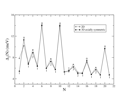
Figure 1: Addition energies $\Delta_{2}(N)$ (meV) as a function of the number of electrons $N$ for a thick QR (solid dots, solid lines) and a strictly 2D QR (open dots, dashed lines). The value of $2S_{z}$ is indicated.

Fig. 1 shows the addition energies $\Delta_{2}(N)$

$$\Delta_{2}(N)=E(N+1)-2E(N)+E(N-1)\;\;\;,$$ (3)

where $E(N)$ is the total energy of the $N$ electron QR, as a function of $N$. It can be seen that the 2D and ‘thick’ -i.e., axially symmetric 3D- models sensibly yield the same results for this observable, a well know result for QD’s.Pi01 For the thick rings, the value of the calculated total spin third component, $2S_{z}$, is also indicated in the figure. We want to point out that in the $N=3$ case, the 2D model configuration is fully polarized $(2S_{z}=3)$. This is due to the fact that the exchange-correlation energy is overestimated by strictly 2D models.Ron99a Fully polarized $N=3$ QR configurations are not an artifact of the LSDFT. As a matter of fact, they have been also found by exact diagonalization methods for some ring sizes and confining potential choices.Zhu05

The gs spin assignments we have found here coincide with those of Ref. Emp01, , although the height of the peaks in $\Delta_{2}(N)$ depends to a large extent on the confining potential. They are related to the relative stability of the electronic shell closures in the ring, which for $N>6$ are substantially different from these of QD’s. In the case of rings, they are mainly governed by the fourfold degeneracy of the non-interacting sp levels with $|l|\neq 0$, and the twofold degeneracy of the non-interacting sp levels with $|l|=0$. This yields the marked shell closures at $N=2,6,10,20$ and 28 with $S_{z}=0$, as well as the $S_{z}=0$ gs found for $N=24$. The $2S_{z}=2$ ground states that regularly appear between them indicate that Hund’s rule is fulfilled by single QR’s.

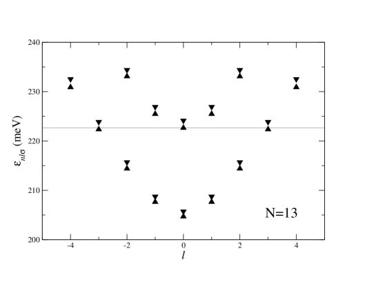
Figure 2: Single particle energy levels (meV) as a function of $l$ for a thick QR with $N=13$. Upward(downward) triangles denote $\uparrow$$(\downarrow$) spin states. The thin horizontal line represents the Fermi energy.

The complex spin structure around $N=13$ deserves some comments. It is due to the occupancy of the second $(s\uparrow)$ state with $l=0$ -this spin structure is missing in other QR calculations that employ a different confining potential.Lin01 Figure 2 displays the sp energies $\varepsilon_{nl\sigma}$ for $N=13$, which are distributed parabolic-like as a function of $l$, each parabola corresponding to a different value of the principal quantum number $n$. This figure explains the filling sequence around $N=13$. For $N=12$, the second $(0\uparrow)$ state is empty, yielding $2S_{z}=2$; for $N=13$ the exchange interaction favors the filling of this state yielding $2S_{z}=3$; for $N=14$, one of the $(\pm 3\downarrow)$ states is filled -they are degenerate-, yielding $2S_{z}=2$ (actually, this many-electron configuration is nearly degenerate with the one in which the $(0\downarrow)$ state is filled instead, which also yields $2S_{z}=2$). For $N=16$, the $(0\downarrow)$ and $(\pm 3\downarrow)$ become populated, producing a fairly strong shell closure.

III.2 Homonuclear quantum ring molecules

We consider first the case of a QRM formed by two identical quantum rings. By analogy with natural molecules, we call them homonuclear QRM. We have calculated their gs structure for $d=$ 2, 4 and 6 nm, and up to $N=32$. For a given electron number $N$, the evolution of the gs (‘phase’) of a QRM as a function of $d$ may be thought of as a dissociation process.Pi01 Within LSDFT, each sp molecular orbital has, as quantum labels, the third component of the spin and of the orbital angular momentum, the parity, and the value of reflection symmetry about the $z=0$ plane. Symmetric states $|S\rangle$ are called bonding states, and antisymmetric states $|AS\rangle$ are called antibonding states.

The energy splitting between bonding and antibonding sets of sp states, $\Delta_{SAS}$, can be properly estimatedPi01 from the energy difference of the antisymmetric and symmetric states of a single electron QRM, $\Delta_{SAS}\sim E(^{2}$$\Sigma^{-}_{u})-$$E(^{2}$$\Sigma^{+}_{g})$ -see below for the notation-, and varies from 24.9 meV at $d=2$ nm (strong coupling), to 1.49 meV at $d=6$ nm (weak coupling). In this range of inter-ring distances, $\Delta_{SAS}$ can be fitted as $\Delta_{SAS}=\Delta_{0}\,e^{-d/d_{0}}$, with $\Delta_{0}=82$ meV and $d_{0}=1.68$ nm. The relative value of the two energies $\hbar\omega_{0}$ and $\Delta_{SAS}$ crucially determines the structure of the molecular phases along the dissociation path.

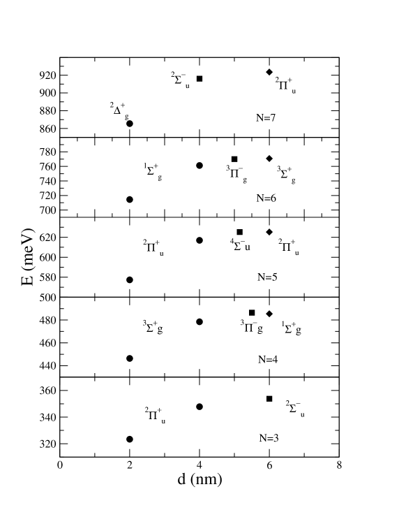
Figure 3: Energy (meV) and gs molecular phases of the homonuclear QRM as functions of the inter-ring distance $d$ for $N=3-7$. For each QRM, different phases are represented by different symbols.

Figure 3 shows the evolution with $d$ of the gs energy and molecular phase of a QRM made of $N=3-7$ electrons. Each configuration is labeled using an adapted version of the ordinary spectroscopy notation,Ron99 namely ${}^{2S+1}L^{\pm}_{g,u}$, where $S$ is the total $|S_{z}|$, and $L$ is the total $|L_{z}|$. The superscript $+(-)$ refers to even (odd) states under reflection with respect to the $z=0$ plane, and the subscript $g(u)$ refers to positive(negative) parity states. To label the molecular sp states we have used the standard convention of molecular physics, using $\sigma,\pi,\delta,\ldots$ if $l=0,\pm 1,\pm 2,\ldots$. Upper case Greek letters are used for the total $|L_{z}|$. Fig. 3 shows that the energy of the molecular phase increases with $d$. This is due to the increase of the energy of the sp bonding states as $d$ increases,Pi01a that dominates over the decrease in Coulomb energy. At larger inter-ring distances, the constituent QR are so apart that eventually the decrease of Coulomb energy dominates and the tendency is reversed. The phase sequences are the same as for double quantum dots,Pi01 although the transition inter-ring distances, which obviously depend on the kind and strength of the confining potential, are different. As for double quantum dots, we have found that the first phase transition of a few-electron QRM is always due to the replacement of an occupied bonding sp state by an empty antibonding one.

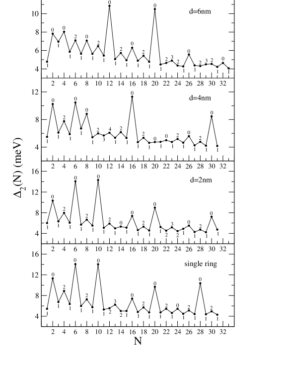
Figure 4: $\Delta_{2}(N)$ for homonuclear QRM with inter-ring distances $d=2,4$, and 6 nm. The addition energies have been offset for clarity. Also shown is the reference spectrum for a single QR. The value of $2S_{z}$ is indicated.

Figure 4 shows the addition spectra for homonuclear QRM up to $N=31$ for the three selected inter-ring distances. Also shown is the reference spectrum of a single QR. The spectra have been offset for clarity. For small $d$ ($\Delta_{SAS}\gg\hbar\omega_{0}$) the spectrum of the QRM is rather similar to a single QR, especially for few-electron systems, with minor changes arising in the $N\sim 12$ and $\sim 24$ regions that will be commented below. It is clear that for $d=2$ nm the two QR’s are electrostatically and quantum-mechanically coupled and behave as a single system. At intermediate distances the spectrum pattern becomes more complex, but at larger distances (e.g. $d=6$ nm), when the QRM molecule is about to dissociate, the physical picture that emerges is rather simple and can be interpreted using intuitive, yet approximate arguments: At large distances ($\Delta_{SAS}\ll\hbar\omega_{0}$), the QR’s are coupled only electrostatically, and most $|S\rangle$ and $|AS\rangle$ states are quasidegenerate. Electron localization in each constituent QR can be achieved combining these states as $(|S\rangle\pm|AS\rangle)/\sqrt{2}$ and as a consequence, the strong $S_{z}=0$ peaks found at $N=12$ and 20 are readily interpreted from the peaks appearing in the single QR spectrum at $N=6$ and 10; the process can be viewed as the symmetric dissociation of the original QRM leading to very robust closed shell single QR configurations. This is also the origin of the QRM $S_{z}=0$ peaks at $N=2$ and 4. In the former case, the QRM configuration corresponds to one single electron being hosted in each constituent QR coupled into a singlet state, and in the latter case, the QRM configuration is viewed as two QR’s, each one occupied by two electrons filling the $1s$ shell.

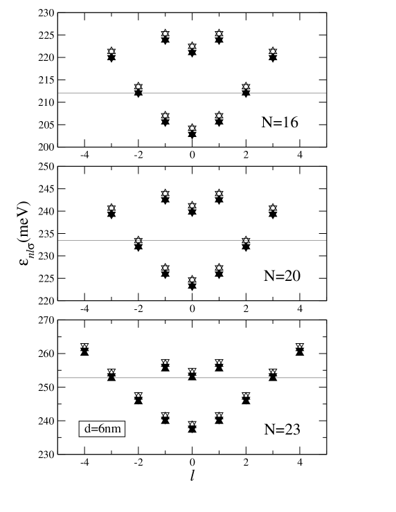
Figure 5: Single particle energy levels (meV) as a function of $l$ for an homonuclear QRM with $d=6$ nm and $N=16$ (top panel), $N=20$ (middle panel), and $N=23$ (bottom panel) . Upward(downward) triangles denote $\uparrow$($\downarrow$) spin states. Open(solid) triangles correspond to antibonding(bonding) states. The thin horizontal line represents the Fermi energy.

At $d=6$ nm, other dissociations display a more complicated pattern, such as $16\rightarrow 8+8$, or $8\rightarrow 4+4$, whose final products are QR’s that fulfill Hund’s rule whereas the actual QRM has $S_{z}=0$. These could be interpreted as rather entangled QRM, ‘harder’ to dissociate, for which a $d=6$ nm inter-ring distance is not large enough to allow for electron localization. The fact is that not only quasidegeneracy of occupied $|S\rangle$ and $|AS\rangle$ states at given $d$ plays a role in this intuitive analysis, but also whether their number is equal or not, so that they may be eventually combined to favor localization. An example of these two different situations is illustrated in Fig. 5, where we show the sp states of the $N=16$, 20 and 23 QRM at $d=6$ nm. In the case of $N=16$ and 23, the filled bonding states near the Fermi level have not filled antibonding partner and are delocalized in the whole volume of the QRM, contributing to the molecular bonding at that distance, whereas all other bonding states can be localized combining them with their antibonding partner: as in natural molecules, some orbitals contribute to the molecular bonding, whereas some others do not.

III.3 Heteronuclear quantum ring molecules

For vertically coupled lithographic double quantum dots, it has been found unavoidable that a slight mismatch is unintentionally introduced in the course of their fabrication from materials with nominally identical constituents quantum wells,Pi01 which is responsible for electron localization as the interdot coupling becomes weaker. This offsets the energy levels in the quantum dots by a certain amount that was there estimated to be up to 2 meV, and this plays a crucial role in the appearance of the addition energy spectra as a function of the coupling strength particularly in the weak coupling limit. A similar picture is also found in coupled self-assembled quantum dots, where strain propagation between adjacent layers of dots often leads to top QD’s of increased size.Le96

Likely, the same fabrication limitations will appear in the case of vertically coupled double quantum rings. Anticipating to this situation, we have carried out a series of QRM calculations in which the double quantum wells have the same width $w$ but slightly different depths, namely $V_{0}\pm\delta$, with $\delta\ll V_{0}$. It can be easily checked that in the weak coupling limit ($2\delta\gg\Delta_{SAS}$), $2\delta$ is approximately the energy splitting between the bonding and antibonding sp states, which would be almost degenerate if $\delta=0$. For this reason we call the mismatch (offset) the quantity $2\delta$.

We have considered two possible values of the mismatch, namely $2\delta=2$ and 4 meV, and have obtained the corresponding addition spectra for up to $N=13$ electrons -according to our previous experience with double quantum dots,Pi01 we expect that the larger differences will arise in few-electron QRM. The results are displayed in Fig. 6. It can be seen that in the strong coupling limit, the effect of the mismatch on the addition energies is negligible, as expected.Pi01 The electrons are completely delocalized in the whole volume of the QRM, and the introduced mismatch is unable to localize them in either of the constituents QR’s.

For the few-electron QRM, which is the more interesting physical situation, we have shown before that the fingerprint of homonuclear character is the appearance, in the weak coupling limit, of the peaks in the addition spectrum corresponding to $N=2$ and 4, as well as the spin assignment $S_{z}=0$. It can be seen from Fig. 6 that in the intermediate regime ($d=4$ nm) the $N=4$ peak still corresponds to a $2S_{z}=2$ configuration, but at larger inter-ring distances, it eventually disappears, yielding an addition spectrum that clearly manifests the heteronuclear character of the QRM and constitutes a clean fingerprint of these kind of configurations.

It is useful to display the dissociation of the QRM representing the $d$ evolution of the sp molecular wave functions, introducing the $z$-probability distribution functionPi01

$${\cal P}(z)=2\pi\int dr\,r\,[u(r,z)]^{2}\;\;\;.$$ (4)

Examples of these probability functions can be seen in Fig. 7, where we show ${\cal P}(z)$ for $N=20$, $2\delta=4$ meV, and $N=8$, $2\delta=2$ meV (deeper well always in the $z<0$ region), each for the chosen three $d$ values. In each panel the probability functions are plotted ordered from bottom to top according to the increasing sp energies. For $N=20$ the final configurations are the closed shell $N=10$, $2S_{z}=0$ QR’s, whereas for $N=8$ the $N=4$, $2S_{z}=2$ Hund’s rule QR configurations emerge.

Finally, we discuss the case of two QR’s of different radii vertically coupled to build an axially symmetric QRM, and study the effect this assymetry has on the addition spectrum (we have discarded a possible disalignment of the QR symmetry axes, as addressing this situation would require a much more demanding full 3D calculationPi04 ). To this end, we have taken for one ring $R_{0}=6$ nm, while for the other one we have kept the same value as before, $R_{0}=5$ nm ($\delta$ is set to zero this case).

We show in Fig. 8 the addition spectra for up to $N=14$ electrons and $d=2$, 4, and 6 nm. It can be seen that in the strong and intermediate coupling cases they are fairly similar to the previous heteronuclear case -and to the homonuclear case as well-, indicating a fairly robust structure of the QRM in these limits. As before, the heteronuclear character clearly shows up in the weak coupling limit, with a peak structure and $S_{z}$ assignments remarkably similar to those discussed in the previous situation with $\delta\neq 0$.

IV Summary and outlook

We have discussed the appearance of the addition energy spectra of homonuclear and heteronuclear quantum ring molecules at zero magnetic field. In particular, we have addressed the addition energy spectrum of QRM from the weak to the strong coupling limits. Fingerprints of homo- and heteronuclear molecular character have been pointed out in the weak coupling limit. As it happened in the study of vertically coupled double quantum dots,Pi01 we believe this may be helpful in the analysis of future experiments on vertical QRM’s.

The present study can be naturally extended to the case of QRM’s submitted to magnetic fields of arbitrary direction. A rich interplay between molecular phases having different isospin is expected to appear as a function of $B$,Anc03 ; Aus04 which might have an observable influence on the Aharonov-Bohm effect and on the far-infrared spectroscopy of nanoscopic QRM’s.

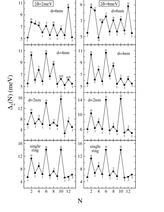
Figure 6: $\Delta_{2}(N)$ for heteronuclear QRM with inter-ring distances $d=2,4$, and 6 nm and mismatch $2\delta=2$ meV (left panels) and $2\delta=4$ meV (right panels). The addition energies have been offset for clarity. Also shown is the reference spectrum for a single QR. The value of $2S_{z}$ is indicated. Note that in some cases two different values of $S_{z}$ have been asigned to the same peak. This means that the corresponding configurations are nearly degenerated.

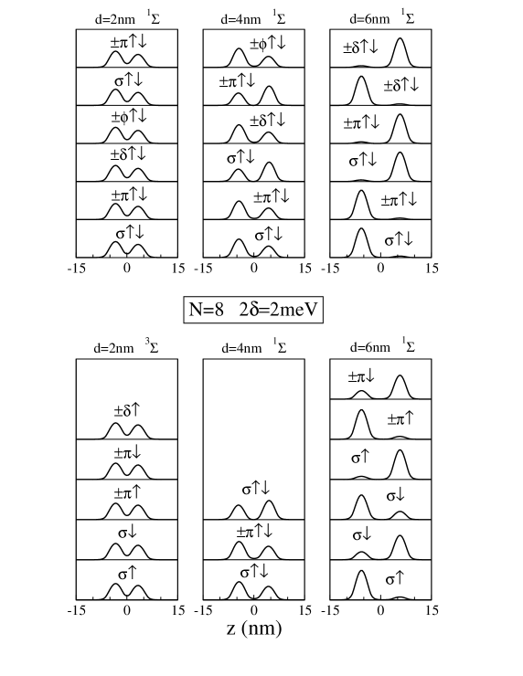
Figure 7: Calculated probability distributions ${\cal P}(z)$ (arbitrary units) as a function of $z$ for heteronuclear QRM’s with $N=20$, $2\delta=4$ meV (top panels), and $N=8$, $2\delta=2$ meV (bottom panels). The corresponding molecular configuration is also indicated.

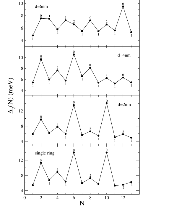
Figure 8: $\Delta_{2}(N)$ for heteronuclear QRM made of QR with different core radii $R_{0}=5$ and $R_{0}=6$ nm, hosting up to $N=14$ electrons and inter-ring distances $d=2,4$, and 6 nm. The addition energies have been offset for clarity. Also shown is the reference spectrum for a single QR. The value of $2S_{z}$ is indicated.

References

- (1) M. Pi, A. Emperador, M. Barranco, F. Garcias, K. Muraki, S. Tarucha, and D.G. Austing, Phys. Rev. Lett. 87, 066801 (2001).
- (2) D.G. Austing, S. Tarucha, H. Tamura, K. Muraki, F. Ancilotto, M. Barranco, A. Emperador, R. Mayol, and M. Pi, Phys. Rev. B 70, 045324 (2004).
- (3) M. Pi, D.G. Austing, R. Mayol, K. Muraki, S. Sasaki, H. Tamura, and S. Tarucha, in Trends in Quantum Dots Research, P. A. Ling, editor p. 1 (Nova Science Pu. 2005).
- (4) M. Rontani, F. Rossi, F. Manghi, and E. Molinari, Solid State Commun. 112, 151 (1999)
- (5) B. Partoens and F.M. Peeters, Phys. Rev. Lett. 84, 4433 (2000); Europhys. Lett. 56, 86 (2001).
- (6) A.E. Hansen, A. Kristensen, S. Pedersen, C.B. Sorensen, and P.E. Lindelof, Phys. Rev. B 64, 45327 (2001).
- (7) A. Lorke, R.J. Luyken, A.O. Govorov, J.P. Kotthaus, J.M. Garcia, and P.M. Petroff, Phys. Rev. Lett. 84, 2223 (2000).
- (8) A. Fuhrer, S. Lüscher, T. Ihn, T. Heinzel, K. Ensslin, W. Wegscheider, and M. Bichler, Nature 413, 822 (2001).
- (9) T. Ihn, A. Fuhrer, T. Heinzel, K. Ensslin, W. Wegscheider, and M. Bichler, Physica E 16, 83 (2003).
- (10) T. Ihn, A. Fuhrer, K. Ensslin, W. Wegscheider, and M. Bichler, Physica E 26, 225 (2005).
- (11) S. Tarucha, D.G. Austing, T. Honda, R.J. van der Hage, and L.P. Kouwenhoven, Phys. Rev. Lett. 77, 3613 (1996).
- (12) S. Tarucha, D.G. Austing, Y. Tokura, W.G. van der Wiel, and L.P. Kouwenhoven, Phys. Rev. Lett. 84, 2485 (2000).
- (13) T. Kuroda, T. Mano, T. Ochiai, S. Sanguinetti, K. Sakoda, G. Kido, and N. Koguchi, Phys. Rev. B 72, 205301 (2005).
- (14) D. Granados, J.M. García, T. Ben, and S.I. Molina, Appl. Phys. Lett. 86, 071918 (2005).
- (15) F. Suárez, D. Granados, M.L. Dotor, and J.M. García, Nanotechnology 15, S126 (2004).
- (16) J.I. Climente, J. Planelles, M. Barranco, F. Malet, and M. Pi, unpublished (2006).
- (17) M. Pi, A. Emperador, M. Barranco, and F. Garcias, Phys. Rev. B 63, 115316 (2001).
- (18) S. Lundqvist, Theory of the Inhomogenous Electron Gas, edited by S. Lundqvist and N. H. March (Plenum, New York, 1983) p. 149.
- (19) J. P. Perdew and A. Zunger, Phys. Rev. B 23, 5048 (1981).
- (20) F. Ancilotto, D.G. Austing, M. Barranco, R. Mayol, K. Muraki, M. Pi, S. Sasaki, and S. Tarucha, Phys. Rev. B 67, 205311 (2003).
- (21) S.S. Li, and J.B. Xia, J. Appl. Phys. 89, 3434 (2001); A. Puente, and Ll. Serra, Phys. Rev. B 63, 125334 (2001); J.I. Climente, J. Planelles, and F. Rajadell, J. Phys.: Condens. Matter 17, 1573 (2005).
- (22) B.C. Lee and C.P. Lee, Nanotechnology 15, 848 (2004).
- (23) A. Emperador, M. Pi, M. Barranco, and E. Lipparini, Phys. Rev. B 64, 155304 (2001).
- (24) M. Rontani, F. Rossi, F. Manghi, and E. Molinari, Phys. Rev. B 59, 10165 (1999).
- (25) J-L. Zhu, S. Hu, Z. Dai, and X. Hu, Phys. Rev. B 72, 075411 (2005).
- (26) J.C. Lin and G.Y. Guo, Phys. Rev. B 65, 035304 (2001).
- (27) N.N. Ledentsov, V.A. Shchukin, M. Grundmann, N. Kirstaedter, J. Böhrer, O. Schmidt, D. Bimberg,V.M. Ustinov, A. Yu. Egorov, A.E. Zhukov, P.S. Kop’ev, S.V. Zaitsev, N.Yu. Gordeev, Zh.I. Alferov, A.I. Borovkov, A.O. Kosogov, S.S. Ruvimov, P. Werner, U. Gösele, and J. Heydenreich, Phys. Rev. B 54, 8743 (1996).
- (28) M. Pi, F. Ancilotto, E. Lipparini, and R. Mayol, Physica E 24, 297 (2004).