Dynamic critical exponents of Swendsen-Wang and Wolff algorithms by nonequilibrium relaxation

Abstract

With a nonequilibrium relaxation method, we calculate the dynamic critical exponent $z$ of the two-dimensional Ising model for the Swendsen-Wang and Wolff algorithms. We examine dynamic relaxation processes following a quench from a disordered or an ordered initial state to the critical temperature $T_{c}$, and measure the exponential relaxation time of the system energy. For the Swendsen-Wang algorithm with an ordered or a disordered initial state, and for the Wolff algorithm with an ordered initial state, the exponential relaxation time fits well to a logarithmic size dependence up to a lattice size $L=8192$. For the Wolff algorithm with a disordered initial state, we obtain an effective dynamic exponent $z_{\rm exp}=1.19(2)$ up to $L=2048$. For comparison, we also compute the effective dynamic exponents through the integrated correlation times. In addition, an exact result of the Swendsen-Wang dynamic spectrum of a one-dimension Ising chain is derived.

1 Introduction

In recent two decades, cluster algorithms have played an important role in statistical physics due to their reduced critical slowing down, improved computational efficiency, and interesting dynamical properties. Among these dynamical properties, the dynamic critical exponent $z$ is the center of attraction, which describes the divergent correlation time.

There are various ways to calculate the dynamic critical exponent $z$, for example, through the exponential decay of the time correlation of a finite system in equilibrium [1, 2], or from the dynamic scaling behavior in nonequilibrium states [3, 4, 5]. In calculating the time correlation in equilibrium, the difficulty is that one can hardly reach a very large lattice. The advantage for computing the dynamic exponent from a nonequilibrium relaxation process is that the finite size effect is more or less negligible, since the spatial correlation length is small in the early stage of the dynamic relaxation. Such a nonequilibrium approach, however, becomes subtle for the cluster algorithms, for the dynamic exponent $z$ is believed to be close to zero. In addition, it is also somewhat controversial in defining a Monte Carlo time for the Wolff algorithm.

In a recent article [6], an attempt is made to estimate the dynamic exponent $z$ of the Wolff algorithm from the finite size scaling behavior in a nonequilibrium state. A vanishing $z$ value is claimed. To our understanding, however, the identification of the dynamic scaling behavior there seems to be not appropriate. On the other hand, although the cluster algorithms are known to be very efficient in reducing critical slowing down with a small dynamic exponent $z$, it has not been rigorously studied what precise values the dynamic exponent $z$ takes for different variants of the algorithms. This is important in theory and application of the cluster algorithms.

In this paper, we will calculate the dynamic exponent $z$ for the Wolff [7] and Swendsen-Wang [8] algorithms, respectively, through the exponential relaxation time and integrated correlation time [9] of the system energy in nonequilibrium relaxation processes. Compared with methods based on computations of time correlation functions in equilibrium, much larger system sizes can be reached in the nonequilibrium dynamic approach, especially in the case of the two-dimensional Ising model, where the system energy in the equilibrium state is known exactly. Compared with the methods in Ref. [6], the system energy in our calculations is self-averaged and thus much less fluctuating in simulations of large lattices.

The paper is organized as follows. In Sec. 2, the general theory of the spectrum of the Monte Carlo dynamics is described, and in Sec. 3, an exact calculation of the spectrum of the one-dimensional Ising chain is formulated. In Sec. 4, simulation setup is discussed in detail, and in Sec. 5, numerical results are presented.

2 Spectrum of Monte Carlo Dynamics

In order to justify our method, we first look at the spectrum of a Markov chain Monte Carlo dynamics [10] and its relation to observables, i.e., the equilibrium and nonequilibrium relaxation functions. Let $W$ be a transition matrix of an irreducible, aperiodic, and reversible Markov chain with an equilibrium (invariant) probability distribution $p$. We have a detailed balance equation between $W$ and $p$,

$$p_{i}W_{ij}=p_{j}W_{ji}.$$ (1)

This equation implies that the following matrix is symmetric:

$$S_{ij}=p_{i}^{1/2}W_{ij}p_{j}^{-1/2},$$ (2)

thus, the eigenvalues $\lambda_{m}$ of $S$ are real. Due to the conservation of the total probability, it can also be shown that $|\lambda_{m}|\leq 1$. Let the eigenvectors of $S$ be $u_{im}$ for eigenvalue $\lambda_{m}$, then the left and right eigenvectors of $W$ is $x_{i}=p_{i}^{1/2}u_{im}$ and $y_{i}=p_{i}^{-1/2}u_{im}$, respectively, such that

$$xW=\lambda_{m}x,\qquad Wy=\lambda_{m}y.$$ (3)

The equilibrium distribution corresponds to $\lambda_{0}=1$, $x^{(0)}=p$, and $y^{(0)}_{i}=1$. The next eigenvalue $\lambda_{1}$ nearest to 1 controls the rate of convergence. We define the exponential relaxation time $\tau$ (in units of one Monte Carlo step or attempt) by $\lambda_{1}=\exp(-1/\tau)$.

We can represent the relaxation of a general observable $Q$ in terms of the initial distribution $p(0)$ or equilibrium distribution $p$ and the eigenspectrum of $S$ as

$$\langle Q(t)\rangle_{p(0)}=\sum_{k}\lambda_{k}^{t}d_{k}c_{k},$$ (4)

$$\langle Q(t)Q(0)\rangle_{eq}=\sum_{k}\lambda_{k}^{t}c_{k}^{2},$$ (5)

where the averages are over the initial distribution and equilibrium distribution, respectively, and

$$c_{k}=\sum_{i}p_{i}^{1/2}Q_{i}\,u_{ik},$$ (6)

$$d_{k}=\sum_{i}p_{i}^{-1/2}p_{i}(0)u_{ik}.$$ (7)

We define the normalized relaxation function $f(t)$ to be linear in $\langle Q(t)\rangle$ or $\langle Q(t)Q(0)\rangle$ such that $f(0)=1$ and $f(\infty)=0$, e.g., $f(t)=(\langle Q(t)\rangle-\langle Q(\infty)\rangle)/(\langle Q(0)\rangle-\langle Q(\infty)\rangle)$. The integrated correlation time is defined as

$$\tau_{\rm int}=\sum_{t=0}^{\infty}f(t).$$ (8)

We note that the integrated correlation time depends not only on the observable $Q$ but also on the dynamics and the full eigen spectrum. The integrated correlation time for the equilibrium correlation and nonequilibrium relaxation is not the same. On the other hand, the exponential relaxation time, defined in the large time limit, $f(t)\sim\exp(-t/\tau)$, is an intrinsic property of the Markov chain. It is the same for both the equilibrium and nonequilibrium situations.

3 Exact Calculation in One Dimension

It is instructive to look at the eigen spectra of the Swendsen-Wang and Wolff dynamics in one dimension (1D). We consider the Swendsen-Wang dynamics in 1D with an open boundary condition. Consider spin $\sigma_{i}$ at a one-dimensional lattice site $i=1$, 2, $\cdots$, $L$, $L+1$. We define the link variable $b_{i}=1-\delta_{\sigma_{i},\sigma_{i+1}}$. The energy of the system is

$$E(\sigma)=-J\sum_{i=1}^{L}\sigma_{i}\sigma_{i+1}=2J\sum_{i=1}^{L}b_{i}+{\rm const}.$$ (9)

We introduce the bond variables $n_{i}=0,1$ representing the absence or presence of a bond in the Swendsen-Wang dynamics, then the joint probability distribution of both the spin and bond is proportional to

$$P(\sigma,n)=\prod_{i=1}^{L}\bigl{[}p\delta_{\sigma_{i},\sigma_{i+1}}\delta_{n_{i},1}+(1-p)\delta_{n_{i},0}\bigr{]},$$ (10)

where $p=1-\exp\bigl{[}-2J/(k_{B}T)\bigr{]}$. The marginal distribution of the spins is given by $\sum_{n}P(\sigma,n)=P(\sigma)=\prod_{i}\exp[-2Jb_{i}/(k_{B}T)]$. The distribution of the bonds is the special case of the Fortuin-Kasteleyn formula, $P(n)=\sum_{\sigma}P(\sigma,n)=p^{N_{b}}(1-p)^{L-N_{b}}2^{L-N_{b}+1}$, $N_{b}=\sum_{i}n_{i}$. The Swendsen-Wang algorithm is to apply alternatively two conditional probabilities, sample bonds given the spins $P(n|\sigma)=P(\sigma,n)/P(\sigma)$, and sample spins given the bonds $P(\sigma|n)=P(\sigma,n)/P(n)$. Instead of using the spin variables, it is more convenient to use the link variable $b_{i}$. In terms of $b_{i}$, the conditional probabilities are simple products:

$$P(n|b)=\prod_{i}f(b_{i},n_{i}),\qquad f=\left(\begin{array}[]{cc}1-p&p\\ 1&0\end{array}\right),$$ (13)

$$P(b|n)=\prod_{i}g(n_{i},b_{i}),\qquad g=\left(\begin{array}[]{cc}1/2&1/2\\ 1&0\end{array}\right).$$ (16)

The transition probability from a given link configuration to another link configuration is

$$W(b\to b^{\prime})=\sum_{n}P(b^{\prime}|n)P(n|b)=\prod_{i}w_{b_{i},b^{\prime}_{i}},\qquad w=\left(\begin{array}[]{cc}\frac{1+p}{2}&\frac{1-p}{2}\\ 1/2&1/2\end{array}\right).$$ (17)

The matrix $w$ has eigenvalues 1 and $p/2$, with left eigenvectors $v^{(1)}=(1,1-p)$ and $v^{(2)}=(1,-1)$, respectively. We note that the full matrix $W$ for the whole system is a direct product from the contribution of each site. Thus, the eigen values of $W$ are $\lambda_{m}=(p/2)^{m}$ [11], with $L!/(m!(L-m)!)$ fold degenerate eigen vectors, $\prod_{i}v^{(k_{i})}(b_{i})$, $k_{i}=1$ or 2, with $L-m$ terms of choices for $k_{i}=1$ and $m$ terms for $k_{i}=2$, where $m=0,1,2,\cdots,L$. The eigenvalue $\lambda_{0}=1$ corresponds to the equilibrium state with a left eigenvector $P(\sigma)$. The next eigenvalue $\lambda_{1}=p/2=\exp(-1/\tau)$ gives the relaxation time. We note that rest of the decay times $\tau/m$ are well-spaced.

It is easy to write down the probability distribution of the domain length since each link evolves independently. Let $P_{l}(t)$ be the probability for observing a domain of a length $l$ with $-$ spins terminated by $+$ spins, then

$$P_{l}(t)=p(b=1,t)\bigl{[}1-p(b=1,t)\bigr{]}^{l-1},$$ (18)

where $p(t)=p(0)w^{t}$ is the probability of the link variable takes the value $1$ at step $t$. Similar result using a continuous time dynamics is given in Ref. [12].

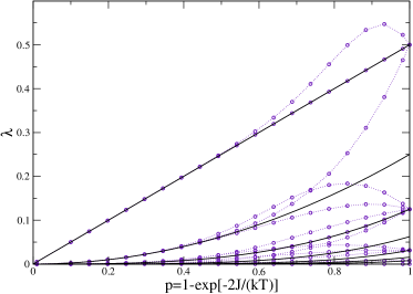
Figure 1: Eigenvalues of the transition matrix of the Swendsen-Wang dynamics in the 1D Ising chain with the open boundary condition (solid lines) and the periodic boundary condition (dotted line with circles) for a lattice size $L=8$.

When a periodic boundary condition is used, we are no longer able to find the eigen spectrum analytically. In Fig. 1, we show the numerical results by diagonalizing the transition matrix on an $L=8$ chain with the periodic boundary condition and compare with the open boundary condition result. We can make several interesting observations. The eigenvalue $\lambda_{1}=p/2$ is always present for both periodic and open boundary conditions for any lattice size $L$. However, we are unable to prove it rigorously. With the periodic boundary condition, the eigen value $p/2$ no longer corresponds to the slowest mode. It seems reasonable that the simple spectrum $(p/2)^{m}$ is a good approximation if the correlation length $\xi\sim\exp(2J/(k_{B}T))$ is much smaller than the system size $L$, thus it is the correct spectrum in the thermodynamic limit. For finite sizes when $\xi$ is comparable to size $L$, the degenerate spectrum splits and rejoins at $T=0$.

4 Simulation Setup

The two-dimensional (2D) Ising model is prepared initially in a random state with a zero magnetization or at the ground state, but evolves at the critical temperature. After a certain time before reaching equilibrium, one can observe an exponential decay of the system energy, which satisfies the following equation:

$$E(t)\approx Ae^{-t/\tau}+E(\infty),$$ (19)

where $\tau$ is the so-called exponential relaxation time. The exponential relaxation time $\tau$ is an intrinsic property of the Monte Carlo algorithm, which is defined by the first excited eigenvalue $\lambda_{1}$ of the transition matrix, and should be independent of the initial states in the simulations. At the transition temperature, the dynamic scaling theory predicts that $\tau$ diverges according to $\tau\sim L^{z_{\rm exp}}$ in the thermodynamic limit. This defines the exponential dynamic critical exponent $z_{\rm exp}$. On the other hand, the integrated correlation time is defined as [9]:

$$\tau_{{\rm int}}=\sum_{t=0}^{\infty}\frac{E(t)-E(\infty)}{E(0)-E(\infty)}.$$ (20)

Similarly, one may define the integrated dynamic critical exponent $z_{\rm int}$ through $\tau_{{\rm int}}\sim L^{z_{\rm int}}$. In order to get a more accurate result, we use the exact value of $E(\infty)$ for the 2D Ising model [13].

The Wolff algorithm exhibits an important difference compared to other algorithms. It only updates the spins belonging to a certain cluster around the seed spin at each Monte Carlo step, while other algorithms sweep the whole lattice. For a fair comparison with the Swendsen-Wang or single-spin-flip algorithms, we need to rescale the Wolff Monte Carlo steps. Specifically, the Monte Carlo time $t^{\prime}$ in the Wolff algorithm should be transformed to $t$

$$t=\sum_{t^{\prime\prime}=1}^{t^{\prime}}\frac{C(t^{\prime\prime})}{L^{d}}$$ (21)

where $t^{\prime}$ or $t^{\prime\prime}$ is the Monte Carlo time step of the Wolff single cluster flip (i.e. the number of clusters flipped so far), $C(t^{\prime\prime})$ is the average size of the cluster at step $t^{\prime\prime}$, and $L^{d}$ ($d=2$) is the total number of spins of the system. $t$ is proportional to the actual CPU time. This newly scaled time $t$ should then be used in Eq. (19) for the exponential relaxation time of the Wolff dynamics.

The integrated correlation time should also be changed to

$$\tau_{\rm int}=\sum_{t^{\prime}=0}^{\infty}\frac{E(t^{\prime})-E(\infty)}{E(0)-E(\infty)}\times\frac{C(t^{\prime})}{L^{d}}.$$ (22)

In the Swendsen-Wang algorithm, there is no complication in the definition of time, we straightforwardly use Eq. (19) and (20) to calculate the dynamic exponent $z_{\rm exp}$ and $z_{\rm int}$.

Our definition of the transformed time $t$ is slightly different from that in Ref. [6]. In Ref. [6], the time $t$ is defined by $t=t^{\prime}C(t^{\prime})$. If $C(t^{\prime})$ takes a scaling form $C(t^{\prime})\propto t^{\prime\alpha}$, two definitions coincide. However, the disadvantage of the definition in [6] is that one needs to assume or know the scaling behavior of the cluster size $C(t^{\prime})$. Our definition of the time $t$ has clear physical meaning, i.e., whenever the number of the flipped spins reaches $L^{d}$, it counts as a unit time.

5 Results

We use the standard Hamiltonian of the two-dimensional Ising model,

$$-\beta H=K\sum_{\langle ij\rangle}\sigma_{i}\sigma_{j}.$$ (23)

Here $\beta=1/(k_{B}T)$ and $K=J/(k_{B}T)$, $k_{B}$ is the Boltzmann constant, $T$ is temperature and $J$ is the interaction energy between two spins. Spins $\sigma_{i}$ take only values $+1$ and $-1$. The site $i$ is on a square lattice with periodic boundary conditions.

Let us start our numerical simulations with the Swendsen-Wang algorithm. To calculate the dynamic exponent $z_{\rm exp}$ of the Swendsen-Wang algorithm, we have used lattices $L=64$, 128, 256, 512, 1024, 2048, 4096, 8192, and each has $2^{24}$, $2^{21}$, $2^{19}$, $2^{17}$, $2^{15}$, $5\times 10^{4}$, $4\times 10^{4}$, $2\times 10^{4}$ runs respectively, and the maximum Monte Carlo time steps of each lattice are 60, 70, 70, 80, 90, 100, 100, 110. Here two different initial temperatures $T=\infty$ and $T=0$ are used in the simulations. The system evolves at the critical temperature. From the exponential decay of the system energy in Eq. (19), one measures the relaxation time $\tau$. The results are plotted on a linear-log scale in Fig. 2. The relaxation times are almost identical for both the hot start and cold start. Obviously, an approximate linear behavior is observed for the lattice size $L>100$ in Fig. 2. In other words, a logarithmic dependence $\tau\sim\ln L$ gives a better fit to the numerical data. If we take into account the data of smaller lattices, the $L$-dependence of the relaxation time could be given by $\tau\sim(\ln L)^{1.2}$.

If we analyze the data in the form of a power-law dependence, we found that the effective exponent $z_{\rm exp}$ decreases continuously with increasing lattice sizes, reaching 0.18 at the largest size simulated. This is shown with a log-log scale in Fig. 3, and it strongly suggests that the relaxation time does not follow a power law with a small but finite exponent. Our extensive data with large system sizes thus agree with the conclusion of Heermann and Burkitt [14]. Previous calculations [8, 15, 16, 17, 18, 19] gave various values ranging from 0.35 to 0.2. This appears to be an effect of finite lattice sizes.

For comparison, we also calculated the integrated relaxation time for the Swendsen-Wang dynamics, it is nearly a constant around $\tau_{\rm int}\approx 3.1$. This implies that $z_{\rm int}\approx 0$, it is consistent with $z_{\rm exp}$.

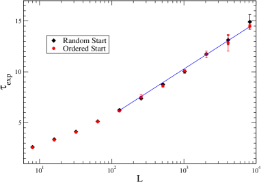
Figure 2: $\tau_{\rm exp}$ versus $L$ in linear-log scale for the 2D Ising model with the Swendsen-Wang dynamics. The diamonds are for random initial configurations, and circles are for the ordered initial state. A straight-line fit gives $\tau_{{\rm exp}}=-3.42+1.98\ln L$.

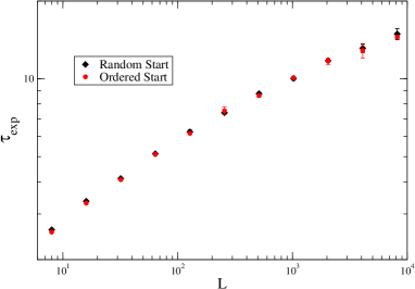
Figure 3: $\tau_{\rm exp}$ versus $L$ in double logarithmic scale for the 2D Ising model with the Swendsen-Wang dynamics.

We now investigate the Wolff dynamics with the fully ordered state at $T=0$ as the initial state, and evolve the system at the critical temperature. The lattice sizes are $L=8$, 16, 32, 64, 128, 256, 512, 1024, 2048, 4096, 8192 with $2^{29}$, $2^{27}$, $2^{24}$, $2^{21}$, $2^{20}$, $2^{20}$, $2^{17}$, $5\times 10^{5}$, $2\times 10^{5}$, $8\times 10^{4}$, $2\times 10^{4}$ independent runs, respectively. The maximum Monte Carlo time steps of each lattice are 80, 100, 150,180, 200, 200, 200, 220, 250, 250, 250. We observe that the dynamic behavior here is very similar to that of the Swendsen-Wang dynamics. As shown in Fig. 4, the correlation time exhibits a logarithmic size dependence even from a relatively small lattice size. The integrated relaxation time is nearly a constant, $\tau_{\rm int}\approx 1.17$ when the lattice size is larger than $256$. This implies that $z_{\rm int}\approx 0$. It is intuitively understandable that the Wolff dynamics starting from a fully ordered state is similar to the Swendsen-Wang dynamics. When the Swendsen-Wang algorithm is initialized in the order state ($T=0$), and then evolves at critical temperature, it forms very large clusters which dominate the evolution of every Monte Carlo step, while other small clusters’ effect can be neglected. Thus its behavior is much like a Wolff algorithm initializing at the ordered state, for it also has a very large cluster dominating the dynamic evolution. For the Swendsen-Wang algorithm with a disordered initial state, our simulations show that the clusters grow rapidly, and the relaxation time is almost the same as that with an ordered initial state.

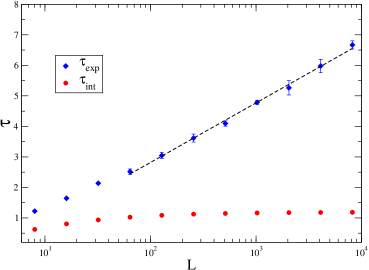
Figure 4: $\tau$ versus $L$ in linear-log scale for the 2D Ising model with the Wolff dynamics starting from an ordered initial state. The diamonds are exponential relaxation times, and a straight-line fit gives $\tau_{{\rm exp}}=1.09+0.85\ln L$. The circles are integrated relaxation times. They reach a steady value near $1.17$ for lattice sizes larger than $256$.

For Wolff dynamics with completely disordered initial states, we have used lattices $L=64$, 128, 256, 512, 1024, 2048 with $2^{24}$, $2^{23}$, $2^{20}$, $2^{17}$, $2^{15}$, $2^{8}$ runs respectively. The maximum Monte Carlo time steps of each lattice are 450, 1337, 4770, 18000, 69910, 300000 in the original time unit of $t^{\prime}$. For the Wolff algorithm with a disordered initial state, the dynamic behavior is rather complicated. In order to have a better comparison of the ordered and disordered initial starts, we present the dynamic relaxation of the system energy for the lattice size $L=2048$ with two different initial conditions in Fig. 5. The figure shows that the dynamic relaxation with a disordered start is much slower.

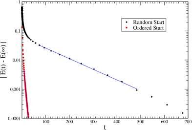
Figure 5: $|E(t)-E(\infty)|$ versus $t$ in log-linear scale for the 2D Ising model with transformed $t$ for the Wolff dynamics. The lattice size is $L=2048$.

In Fig. 6, $\tau_{\rm exp}$ and $\tau_{\rm int}$ are plotted as functions of the lattice size $L$ in log-log scale. For $\tau_{\rm exp}$, an approximate power-law behavior is observed, and from large lattice sizes one derives a dynamic exponent $z_{\rm exp}\approx 1.0$. To obtain a better value of $z$, one may consider corrections to scaling. For example, assuming $\tau_{\rm exp}\sim L^{z}(1+c/L^{\delta})$, the fitted dynamic exponent is $z_{\rm exp}=1.19(2)$. Similarly we estimate $z_{\rm int}=0.29(3)$ from $\tau_{\rm int}$. $z_{\rm exp}$ is much larger than the results obtained in equilibrium correlation functions [15]. Both of these values are quite different from that reported in Ref. [6], where it is concluded that the exponent $z$ is very close to zero.

To understand the difference between our analysis and that in Ref. [6], we have also performed the scaling plot of Fig. 1 in Ref. [6] with our numerical data. Indeed, the scaling collapse is observed for large lattices. According to our scaling analysis, however, a dynamic exponent $z\approx 1.7$ should be extracted. Following the definition in Ref. [6], $t=t^{\prime}\langle C(t^{\prime})\rangle/L^{d}$ with $t^{\prime}$ being the Monte Carlo time step of the Wolff single cluster flip, and then $\tau=\tau^{\prime}\langle C\rangle/L^{d}$. Assuming that $\langle C\rangle$ behaves like susceptibility, i.e., $\langle C\rangle\sim L^{\gamma/\nu}$, one may deduce $z=z^{\prime}-(d-\gamma/\nu)=z^{\prime}+2(Y_{H}-d)$. In Ref. [6], this is written as $z=z^{\prime}-(2Y_{H}-d)$. Together with other inconsistent formulations, a dynamic exponent $z\sim 0$ is derived.

In numerical simulations in equilibrium, one tends to conclude that the dynamic exponent $z$ of the Wolff algorithm is close to zero. This is in agreement with our results from the dynamic relaxation starting from an ordered initial state. Compared with the dynamic relaxation of the Wolff algorithm with an ordered initial state, why does the dynamic relaxation with a disordered initial state show an anomalous behavior? Our conjecture is that the eigenvalues $\lambda_{m}$ of the transition matrix of the Wolff algorithm are rather dense. Within a rather long time, the contribution of the higher eigenvalues to the dynamic observable will not be suppressed in the dynamic relaxation starting from a disordered state. The dynamic exponent measured in this paper and in Ref. [6] is actually an effective one. This also explains why the dynamic exponent extracted from the exponential decay of the system energy is somewhat smaller than that from the dynamic scaling behavior in the relatively short time regime in Ref. [6]. Our numerical simulations and data analysis actually show that if possible, one should avoid starting the simulations with the Wolff algorithm from a disordered state.

Finally, we should mention that for the dynamic relaxation of the Wolff algorithm with a disordered initial state, it is hard to measure the relaxation time $\tau_{\rm exp}$ in an extremely long time regime where the contribution of the higher eigenvalues is already suppressed, since $|E(t)-E(\infty)|$ is too much fluctuating.

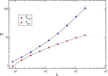
Figure 6: $\tau$ versus $L$ in double logarithmic scale for the 2D Ising model with the Wolff algorithm starting from disordered states. The diamonds are exponential relaxation times $\tau_{\rm exp}$. The circles are integrated relaxation times.

6 Conclusion

In summary, we have computed both the exponential and integrated relaxation times for the Wolff and Swendsen-Wang algorithms, with both disordered and ordered initial states. For the Swendsen-Wang dynamics, the exponential relaxation time shows a logarithmic dependence on the lattice size $L$ for both initial states, while the integrated relaxation time tends to a constant. This is a strong evidence that $z_{\rm exp}=0$ for the Swendsen-Wang algorithm. For the Wolff dynamics with an ordered initial state, the results are similar to those of the Swendsen-Wang dynamics. For the Wolff dynamics with a disordered initial state, however, the dynamic relaxation is very slow, and it takes a very long time to approach equilibrium. If one measures the relaxation time $\tau_{\rm exp}$ in a reasonable time regime in the simulations, an effective dynamic exponent $z_{{\rm exp}}=1.19(2)$ is obtained.

References

- [1] J. K. William, J. Phys. A 18, 49 (1985).
- [2] S. Wansleben and D. P. Landau, Phys. Rev. B 43, 6006 (1991).
- [3] Z. B. Li, L. Schülke, and B. Zheng, Phys. Rev. Lett. 74, 3396 (1995).
- [4] H. J. Luo, L. Schülke, and B. Zheng, Phys. Rev. Lett. 81, 180 (1998).
- [5] B. Zheng, Int. J. Mod. Phys. B 12, 1419 (1998).
- [6] S. Gündüç, M. Dilaver, M. Aydin, and Y. Gündüç, Comp. Phys. Comm. 166, 1 (2005); cond-mat/0409696.
- [7] U. Wolff, Phys. Rev. Lett. 62, 361 (1989).
- [8] R. H. Swendsen and J.-S. Wang, Phys. Rev. Lett. 58, 86 (1987).
- [9] D. P. Landau and K. Binder, A Guide to Monte Carlo Simulations in Statistical Physics, (Cambridge, 2000).
- [10] D. Aldous and J. Fill, Reversible Markov chains and random walks on graphics, http://www.stat.berkeley.edu/users/aldous/RWG/book.html, Chap. 3.
- [11] R. C. Brower and P. Tamayo, Phys. Rev. Lett., 62, 1087 (1989).
- [12] P. L. Krapivsky, J. Phys. A: Math. Gen. 37, 6917 (2004).
- [13] A. E. Ferdinand and M. E. Fisher, Phys. Rev. 185, 832 (1969).
- [14] D. W. Heermann and A. N. Burkitt, Physica A, 162, 210 (1990).
- [15] U. Wolff, Phys. Lett. B 228, 379 (1989).
- [16] C. F. Baillie and P. D. Coddington, Phys. Rev. B 43, 10617 (1991); P. D. Coddington and C. F. Baillie, Phys. Rev. Lett. 68, 962 (1992).
- [17] W. Kerler, Phys. Rev. D 47, R1285 (1993); ibid. 48, 902 (1993).
- [18] J.-S. Wang, O. Kozan, and R. H. Swendsen, Phys Rev E 66, 057101 (2002). J.-S. Wang, in Monte Carlo and Quasi-Monte Carlo Methods 2000, p.141, edited by K.-T. Fang, F. J. Hickernell, and H. Niederreiter, (Springer, Berlin, 2002).
- [19] G. Ossola and A. D. Sokal, Nucl.Phys. B 691, 259 (2004); J. Salas and A. D. Sokal, J. Stat. Phys. 98, 551 (2000); cond-mat/9904038v1.