Impurity effects on optical response in a finite band electronic system coupled to phonons

Abstract

The concepts, which have traditionally been useful in understanding the effects of the electron–phonon interaction in optical spectroscopy, are based on insights obtained within the infinite electronic band approximation and no longer apply in finite band metals. Impurity and phonon contributions to electron scattering are not additive and the apparent strength of the coupling to the phonon degrees of freedom is substantially reduced with increased elastic scattering. The optical mass renormalization changes sign with increasing frequency and the optical scattering rate never reaches its high frequency quasiparticle value which itself is also reduced below its infinite band value.

I Introduction

Many of the physical insights that have guided the interpretation of data on effects of the electron–phonon interaction in metals are based on an infinite band model with a constant featureless electronic density of states (EDOS) mars-book . In the eighties there appeared several studies, mainly motivated by the physics of the A15 compounds, which took account of energy dependence in the EDOS around the chemical potential mitrovic83 ; pickett82 ; mitrovic-thesis81 . Band structure calculations for the A15 showed peaks in the EDOS with variations on the energy scale of $50$ meV. A variety of experiments also showed sensitivity of properties to disorder. For example, disordered Mo₃Ge has a higher value of superconducting critical temperature than its crystalline counterpart. This is naturally explained if the chemical potential in ordered metallic Mo₃Ge falls in a valley of the EDOS. Radiation damage then fills this valley and leads to an increase in EDOS at the Fermi energy and a higher value of T_c.

More recently several authors have considered a different but related effect, namely a finite band cappelluti03 ; dogan03 ; knigavko05 ; knigavko05-2 . One experimental realization of this situation is the fulleride compounds M₃C₆₀ ($M$ – an alkali metal), where band structure calculations gelfand94 show narrow band with the width $W$ of the order of 1 eV, while the phonon spectrum extends up to about 200 meV in some cases. Physical consequences brought about by the finite band can be studied in the frame of a simplified (particle–hole symmetric) model with a constant $N_{0}$ with a cut off applied at $\pm W/2$ where $W$ the band width related to $N_{0}$ by $N_{0}=1/W$. A somewhat surprising result of such studies is that, even for rather wide bands ($W$ of order a few eV) certain aspects associated with the effect of the electron–phonon interaction are profoundly modified as compared to the corresponding infinite band behavior. For example, in an infinite band with constant electronic density of states, the electron–phonon interaction leaves $N_{0}(\omega)$ unaltered and no phonon structure appears in the dressed normal state EDOS. To see phonon structure it is necessary to go to the superconducting state which develops a gap and consequently a non constant EDOS. However if a cut off is applied to the constant $N_{0}(\omega)$, then phonon structure appears in the dressed quasiparticle density of states as it does in the superconducting state and also in any case when EDOS is non constant around the Fermi energy. The phonon structure which appears in the dressed EDOS is surprisingly significant in magnitude even for modest value of the electron–phonon mass renormalization parameter $\lambda$. Mathematically the self energy must be solved for self consistently when a finite band cut off is introduced. This contrasts with the infinite band case where the bare Green’s function can be employed in the self energy expression englesberg63 . Self consistency leads to a smearing of the band edge region as well as a widening of the band. As the total number of states in the electronic density of state must remain constant, this transfer of spectral weight to higher energies beyond the bare EDOS cut off, implies that it must correspondingly be reduced at smaller energies and the details of this reduction depend significantly on the phonon energy scale and coupling strength to the various phonon modes. The effect of widening of a finite electronic band due to the electron–phonon interaction has been observed and discussed previously by Liechtenstein et al liechtenstein96 in the context of fulleride compounds.

There are many qualitative changes in electron–phonon renormalization effects which have their origin in finite bands. For example the real part of the electronic self energy $\Sigma_{1}(\omega)$ for $\omega\geq 0$ is everywhere negative in an infinite band and decays to zero beyond a few times the maximum phonon energy, which we denote $\omega_{D}$. Thus the electronic effective mass is always increased by the electron–phonon interaction and returns to its bare mass value from above at a few times $\omega_{D}$. By contrast for a finite band, as described in Ref. cappelluti03, , $\Sigma_{1}(\omega)$ change sign as $\omega$ increases and the renormalized mass at high $\omega$ can actually be smaller than the bare band mass. This is an example of qualitative change brought about in the electronic self energy by finite band effects. Others are described in the recent paper of Cappelluti and Pietronero cappelluti03 , who also considered the effect of impurities.

In this paper we consider optical properties with particular emphasis on the combined effect of temperature and impurity scattering in a finite band electron–phonon system. In Section II we provide a brief summary of the formalism needed to compute the electron self energy $\Sigma$ vs $\omega$ for a system of electrons coupled both to phonons and to impurities. We also present analytic formulas which apply in the non selfconsistent approximation. They will prove useful for interpretation of the numerical results. The optical conductivity without vertex corrections follows from the Kubo formula for the current–current correlation function. The optical self energy, or the memory function, is introduced and related to the complex optical conductivity $\sigma(\omega)$. We summarize some known approximate but analytic formulas for the optical scattering rate and effective mass renormalization which have been found useful in past studies related to infinite (very wide) electronic bands. These formulas appropriately modified in the context of finite bands are applied to obtain a description of the non selfconsistent approximation, which provide insight into the various features found in numerical solution of the full equations. Two models for the electron–phonon spectral density $\alpha^{2}F(\omega)$ are introduced. For definiteness both are based on the specific phonon spectrum of $K_{3}C_{60}$. One consists of three delta functions suitably chosen to mimic the real spectrum while the other one uses truncated Lorentzians instead of delta functions to help understand the modification brought about when the extended nature of real spectra is accounted for. In Section III we describe results for the case of a rather wide band and the three delta function model for $\alpha^{2}F(\omega)$ with a modest value of $\lambda=0.71$. We start with a discussion of the dressed electronic density of states with emphasis on temperature and impurity effects. Then the memory function is analyzed and compared with the quasiparticle self energy, the differences arising from finite band effects are emphasized. In Section IV we present the results for an extended electron–phonon spectrum, increasing the spectral $\lambda$ and decreasing the width of the band. Section V is our conclusions.

II Formalism

II.1 The electronic self energy and the renormalized EDOS

The central quantity of our problem is the electronic self energy $\Sigma(z)=\Sigma_{1}(z)+{\rm i}\Sigma_{2}(z)$. It is calculated from the Migdal equations formulated in the mixed real–imaginary axis representation cappelluti03 ; marsiglio88 :

$$\Sigma(z) = \Gamma\,\eta(z)+T\sum_{m=-\infty}^{+\infty}\lambda(z-{\rm i}\omega_{m})\eta({\rm i}\omega_{m})$$ (1)

$$+ \int_{0}^{\infty}{\rm d}\omega\,\alpha^{2}F(\omega)\left\{\left[f(\omega-z)+n(\omega)\right]\eta(z-\omega)+\left[f(\omega+z)+n(\omega)\right]\eta(z+\omega)\right\},$$

$$\lambda(z) = \int_{0}^{\infty}{\rm d}\omega\,\alpha^{2}F(\omega)\frac{2\omega}{\omega^{2}-z^{2}},$$ (2)

$$\eta(z) = \int_{-\infty}^{\infty}{\rm d}\xi\,\frac{N_{0}(\xi)}{N_{0}(0)}\frac{1}{z-\xi-\Sigma(z)},$$ (3)

where $\omega_{m}=\pi T(2m-1),$ $m\in Z$ are the fermionic Matsubara frequencies, and $f(\omega)$ and $n(\omega)$ are the Fermi and Bose distribution functions respectively. The electron–phonon interaction is specified in terms of the electron–phonon spectral function $\alpha^{2}F(\omega)$ (the Eliashberg function). The parameter $\Gamma$, which has the meaning of an impurity scattering rate, specifies the strength of the interaction with impurities. The variable $z$ in eqs. (1)–(3) can assume arbitrary complex values. Description of spectroscopic experiments requires knowledge of the retarded electronic self energy at real frequencies, which corresponds to solutions with $z=\omega+{\rm i}0^{+}$. A fast and stable numerical procedure for this purpose was proposed by Marsiglio et al marsiglio88 . It starts with computing the solutions for $\Sigma(z)$ on the imaginary axis, at $z={\rm i}\omega_{m}$, where eq. (1) is simpler. Then, the function $\eta({\rm i}\omega_{m})$ is used to set up an iterative procedure to find $\Sigma(\omega+i0^{+})$ just above the real axis.

The quantity $N_{0}(\xi)$ appearing in Eq. (3) is the bare EDOS. In this paper we use for it the following simple model:

$$N_{0}(\xi)=N_{0}\Theta\left(W/2-|\xi|\right),$$ (4)

where $W$ is the bare band width and $\Theta(x)$ is the step function. The constant $N_{0}$ is fixed by normalization: $N_{0}=1/W$. In this paper we retain particle-hole symmetry for simplicity, with the chemical potential at the center of the band, $\mu=0$. In the clean case it was shown knigavko05 that the main characteristic features appearing in the electronic self energy and the memory function due to the finite band width, do not depend significantly on details of the bare electronic band.

The renormalized density of electronic states, or density of states for quasiparticles, is defined by

$$N(\omega)=\int\nolimits_{-\infty}^{+\infty}d\xi N_{0}(\xi)A(\xi,\omega).$$ (5)

Here

$$A(\xi,\omega)=-\mathop{\rm Im}G_{ret}(\xi,\omega)/\pi$$ (6)

is the electronic spectral density and the retarded Green’s function $G_{ret}(\xi,\omega)$ is defined by the relation

$$\left[G_{ret}(\xi,\omega)\right]^{-1}\equiv\left(\left[G_{0}(\xi,z)\right]^{-1}-\Sigma(z)\right)_{z=\omega+i0^{+}}$$ (7)

with $G_{0}(\xi,z)=1/(z-\xi)$ being the free electron Green’s function. The renormalized quasiparticle can be expressed in terms of the function $\eta=\eta_{1}+{\rm i}\eta_{2}$  of Eq. (3) as follows $N(\omega)/N_{0}(0)=-\eta_{2}(\omega)/\pi$.

The renormalized density of states $N(\omega)$ is a very important quantity. It features various signatures of the interaction of electrons with phonons and impurities. Note that in the infinite electronic band approximation with flat bare EDOS the renormalized EDOS $N(\omega)$ remains constant and does not carry any physical information. In the present context of a finite band, $N(\omega)$ for electron–phonon system has been studied recently by Doğan and Marsiglio dogan03 at $T=0$ and by Knigavko and Carbotte knigavko05 at finite temperatures. Below we emphasize the analysis of the combined effect of both phonons and impurities. We find that knowledge of the features of the renormalized EDOS helps to understand better the behavior of the other spectroscopic quantities such as the memory functions, which are related to the optical response. The renormalized EDOS $N(\omega)$ itself is a measurable quantity and can be directly probed by tunneling spectroscopy or angle-integrated photoemission spectroscopy reinert00 ; chainani00 ; reinert03 . The accuracy of the latter technique has increased dramatically in recent years and properties of both new and traditional materials have been scrutinized. It has been argued in Ref. knigavko05-2, that normal state boson structure should be detectable in such experiments for metals with electronic band width of order a few eV.

Let us return to the electronic self energy. For the purpose of the following discussion we present the general Eq. (1) for the values of the argument just above the real axis, namely $z=\omega+i0^{+}$ and at temperature $T=0$ (note that henceforth we will use real axis variable, such as $\omega$, as shorthand for $\omega+i0^{+}$). Separating the real and imaginary parts of $\Sigma$ we obtain the following expressions:

$$\Sigma_{1}(\omega) = \Gamma\,P\!\!\int_{-\infty}^{\infty}\frac{d\omega^{\prime}}{\omega-\omega^{\prime}}\frac{N(\omega^{\prime})}{N_{0}(0)}+2\omega\,P\!\!\int_{0}^{\infty}d\omega^{\prime}\frac{N(\omega^{\prime})}{N_{0}(0)}\int_{0}^{\infty}d\Omega\frac{\alpha^{2}F(\Omega)}{\omega^{2}-(\omega^{\prime}+\Omega)^{2}},$$ (8)

$$\Sigma_{2}(\omega) = -\pi\left[\Gamma\frac{N(\omega)}{N_{0}(0)}+\int_{0}^{\omega}d\Omega\alpha^{2}F(\Omega)\frac{N(\omega-\Omega)}{N_{0}(0)}\right],$$ (9)

where the symbol $P$ in Eq. (8) means that in the divergent integrals over $\omega^{\prime}$ the Cauchy principal value has to be taken. Note that the self consistent nature of this equations is now masked. On the right hand side of Eqs. (8) and (9) the self energy enters only via the renormalized EDOS $N(\omega)$.

The quasiparticle mass renormalization is defined by the relation:

$$\lambda^{(eff)}_{qp}=-\lim_{\omega\rightarrow 0}{\rm d}\Sigma_{1}{(\omega})/{\rm d}\omega.$$ (10)

From Eq. (8) we find that it is given by

$$\lambda^{(eff)}_{qp} = \Gamma\,P\!\!\int_{-\infty}^{\infty}\frac{d\omega}{\omega}\frac{N^{\prime}(\omega)}{N_{0}(0)}+2\int_{0}^{\infty}d\Omega\alpha^{2}F(\Omega)\int_{0}^{\infty}\frac{d\omega}{(\omega+\Omega)^{2}}\frac{N(\omega)}{N_{0}(0)},$$ (11)

where $N^{\prime}(\omega)\equiv{\rm d}N(\omega)/{\rm d}\omega$ is the derivative of the renormalized EDOS. For an infinite band with a constant $N(\omega)$ we recover the known result. The second term on the right hand side of Eq. (11) reduces to $\lambda=2\int_{0}^{\infty}d\Omega\alpha^{2}F(\Omega)/\Omega$, the usual expression for the mass renormalization due to electron–phonon interaction, while the first term, which represents the effect of the elastic scattering from impurities, vanishes. In the case of an energy dependent EDOS impurities produce a finite contribution to the quasiparticle mass renormalization. Our subsequent numerical analysis shows that for a finite band $N^{\prime}(\omega)$ is a decreasing function of $\omega$ for $\omega>0$ in large intervals, which become especially substantial if $\omega_{D}\ll W$ [remember that $N(-\omega)=N(\omega)$ because we consider the half filling case]. This makes the impurity contribution to $\lambda^{(eff)}_{qp}$ negative and opposite in sign to the phonon contribution. Therefore, in a finite electronic band the increased elastic scattering results in the apparent decrease of the magnitude of the electron–phonon interaction, as specified by $\lambda^{(eff)}_{qp}$.

In this paper we solve the self consistent equations for the self energy numerically. To better understand the trends observed in our numerical results it is helpful to have analytic, though maybe not exact, expressions for the self energy. We found that a useful approximation is to replace the renormalized EDOS $N(\omega)$ in Eq. (8), (9) and (11) with the bare EDOS $N_{0}(\omega)$, given in the model we consider by a constant equal to $N_{0}(0)$ with cutoff at the bare band edge $W/2$ (see Eq. (4)). This approximation amounts to disregarding the self consistency, while keeping track of the finite width of the band. It is expected, and we confirm this in the following Section, that this approximation is good at small frequencies $\omega$ as long as the characteristic phonon frequency is much smaller than the band width $W$. Moreover, this non selfconsistent approximation allows us to obtain a simple estimate for the characteristic frequency $\bar{\omega}_{qp}$ of a finite electronic band, when the real part of the self energy $\Sigma_{1}(\omega)$ changes sign. Deficiencies of the non selfconsistent approximation are discussed later. The non selfconsistent results have the form:

$$\Sigma_{1}^{(ns)}(\omega) = \Gamma\ln\left|\frac{\omega+W/2}{\omega-W/2}\right|+\int_{0}^{\infty}{\rm d}\Omega\,\alpha^{2}F(\Omega)\ln\left|\frac{\omega-\Omega}{\omega+\Omega}\,\frac{\omega+W/2+\Omega}{\omega-W/2-\Omega}\right|,$$ (12)

$$\Sigma_{2}^{(ns)}(\omega) = -\pi\left[\Gamma\Theta(W/2-|\omega|)+\int_{0}^{\omega}{\rm d}\Omega\,\alpha^{2}F(\Omega)\Theta(W/2-|\omega-\Omega|)\right],$$ (13)

$$\lambda^{(ns)}_{qp} = -2\frac{\Gamma}{W/2}+2\int_{0}^{\infty}d\Omega\frac{\alpha^{2}F(\Omega)}{\Omega}\frac{1}{1+\Omega/(W/2)}.$$ (14)

These equations, while not exact, reduce to the well known infinite band results in the limit $W\rightarrow\infty$ and show the modifications brought about by a finite band. Note in particular that when no impurities are present the mass renormalization is always reduced over its infinite band value and that the quasiparticle scattering rate $\tau^{-1}_{qp}(\omega)\equiv-2\Sigma_{2}(\omega+i0^{+})$ drops to zero for $\omega>W/2+\omega_{D}$ instead of remaining constant as in the infinite band case (we remind that $\omega_{D}$ denotes the maximum phonon frequency in $\alpha^{2}F(\Omega)$).

II.2 Optical response

For characterization of the optical response the quantity of interest is the memory function, which is the optical counterpart of the self energy. The memory function $M(\omega)=M_{1}(\omega)+iM_{2}(\omega)$ appears explicitly in the following expression for the complex optical conductivity $\sigma(\omega)=\sigma_{1}(\omega)+{\rm i}\sigma_{2}(\omega)$:

$$\sigma(\omega)=\frac{2S}{\pi}\frac{1}{M(\omega)-i\omega},$$ (15)

which is also called in the literature the extended Drude formula shulga1 ; allen1 ; optics-1 ; optics-2 ; tanner1 . In this equation $S$ is the optical sum defined by the integral

$$S=\int_{0}^{+\infty}\sigma_{1}(\omega)d\omega.$$ (16)

For the infinite and flat electronic band it was shown by Allenallen04 that in the limit $\omega\rightarrow 0$ the memory function and the self energy are closely related, namely: $M_{1}(0)=-2\Sigma_{2}(0)$ and $M_{2}(0)=\Sigma_{1}(0)$. This is one of the reasons why the real part of the memory function can be identified as the optical scattering rate, $M_{1}(\omega)\equiv\tau_{op}^{-1}(\omega)$. On the other hand, the imaginary part of the memory function is usually related to the frequency dependent optical mass renormalization, $M_{2}(\omega)\equiv-\omega\lambda_{op}(\omega)$. The memory function can easily be found if the conductivity is known. Indeed from Eq. (15) it follows that

$$\tau_{op}^{-1}(\omega) = \frac{2S}{\pi}\frac{\sigma_{1}(\omega)}{\sigma_{1}^{2}(\omega)+\sigma_{2}^{2}(\omega)},$$ (17)

$$-\omega\lambda_{op}(\omega) = \omega-\frac{2S}{\pi}\frac{\sigma_{2}(\omega)}{\sigma_{1}^{2}(\omega)+\sigma_{2}^{2}(\omega)}$$ (18)

and these are the relations that we used in our numerical work presented below.

The optical conductivity was obtained using linear response theory, neglecting vertex corrections. The details were described previously elsewhere knigavko05 , and here we just write down the expression for the real part of the conductivity:

$$\sigma_{1}(\omega) = \frac{2\pi e^{2}}{\hbar^{2}}\int_{-\infty}^{+\infty}{\rm d}\xi N_{v}(\xi)\int_{-\infty}^{\infty}{\rm d}\omega^{\prime}A\left(\xi,\omega^{\prime}\right)A\left(\xi,\omega^{\prime}+\omega\right)\frac{f\left(\omega^{\prime}\right)-f(\omega^{\prime}+\omega)}{\omega},$$ (19)

and point out that the corresponding imaginary part was computed as the Hilbert transform of the real part, based on the the Kramers–Kronig relations. In Eq. (19) $N_{v}(\xi)\equiv N_{0}(\xi)v_{\xi}^{2}$ where $v_{\xi}^{2}$ is the averaged over the Brillouin zone the square of the group velocity defined for a general dispersion in Ref. marsiglio90, . In the following discussion of the optical response and in the numerical calculations of this paper we assume that the system is isotropic and use for $v_{\xi}^{2}$ the expression $v_{\xi}^{2}=\frac{2\hbar^{2}}{mD}\left(\frac{W}{2}+\xi\right)$, derived from the quadratic dispersion of free electrons with lower band edge at $\xi=-W/2$ ($D$ is the number of spatial dimensions, $m$ the free electron mass). It is useful to introduce the optical effective mass renormalization as

$$\lambda^{(eff)}_{op}=\lambda_{op}(\omega=0),$$ (20)

which is the quantity to be compared with the quasiparticle effective mass renormalization $\lambda^{(eff)}_{qp}$ of Eq. (10). We will see that complete numerical results indicate that these two quantities are not the same in a finite band. Another important quantity that we will discuss below is the optical scattering rate at the Fermi level, $\tau_{op}^{-1}(\omega=0)$.

As we have done for the self energy it is helpful in understanding the complete numerical results, that will be presented in the following sections, to have simple although approximate analytic expressions for the optical quantities with which to compare. It is not feasible to obtain a simple accurate expression for the optical scattering rate in the general case, and even our model of bare EDOS with sharp cutoffs (see Eq. (4)) do not provide enough simplifications for this purpose. We decided therefore to make use of the existing expressions, valid for the infinite band. Historically, based on second order perturbation theory for the electron–phonon system Allen allen71 was the first to provide such an equation valid at zero temperature in the infinite flat band case. A generalization to finite temperature was made by Shulga et al shulga91 using a very different method which starts with the Kubo formula and makes approximations to get the same result as Allen when $T\rightarrow 0$ limit is taken. On the other hand Mitrović and Fiorucci mitrovic85 and Mitrović and Perkowitz mitrovic84 have generalized Allen’s original work to include the possibility of an energy dependent electronic density of states. They considered only zero temperature. Very recently Sharapov and Carbotte sharapov05 have provided a finite temperature extension based on the Kubo formula. Such formulas have also been used recently in analysis of data hwang05 ; dordevic05 and in comparison with more complete approaches carbotte05 ; schachinger03 . The formulas for the optical effective mass and scattering rate, which are suitable for our forthcoming discussion, are those for $T=0$. They are given in Refs. mitrovic85, and mitrovic84, and here we reproduce them for the reader’s convenience:

$$\lambda_{op}(\omega) = \frac{2\Gamma}{\omega^{2}}P\int_{0}^{\infty}{\rm d}\omega^{\prime}\frac{N(\omega^{\prime})}{N_{0}(0)}\ln\left|\frac{\omega^{\prime 2}}{\omega^{\prime 2}-\omega^{2}}\right|+\frac{2}{\omega^{2}}\int_{0}^{\infty}{\rm d}\Omega\,\alpha^{2}F(\Omega)P\int_{0}^{\infty}{\rm d}\omega^{\prime}\frac{N(\omega^{\prime})}{N_{0}(0)}\ln\left[\frac{(\omega^{\prime}+\Omega)^{2}}{(\omega^{\prime}+\Omega)^{2}-\omega^{2}}\right],$$ (21)

$$\tau_{op}^{-1}(\omega) = \frac{2\pi\Gamma}{\omega}\int_{0}^{\omega}{\rm d}\omega^{\prime}\frac{N(\omega^{\prime})}{N_{0}(0)}+\frac{2\pi}{\omega}\int_{0}^{\infty}{\rm d}\Omega\,\alpha^{2}F(\Omega)\int_{0}^{\omega-\Omega}{\rm d}\omega^{\prime}\frac{N(\omega^{\prime})}{N_{0}(0)},$$ (22)

where the symbol $P$ means, as usual, that the $\omega^{\prime}$ integrals are calculated as the principal Cauchy values. In the above equations $N(\omega)$ is the renormalized EDOS that fully incorporates the self consistent electronic self energy. To grasp the finite band effects in the memory function we intend to replace $N(\omega)$ with the bare EDOS $N_{0}(\omega)$ from Eq. (4) similarly to our approach to the derivation of Eqs. (12)–(13) for the non self consistent self energy. Note however that in order to arrive at Eqs. (21) and (22) it is necessary to assume mitrovic85 that $N_{v}(\xi)$ is constant and extends to infinity, i. e. no cut off is applied to it. This means that after the proposed replacement effectively only finite band effects originating in the self energy are included in the optical quantities and the resulting approximate formulae are not expected to be quantitatively correct for all frequencies $\omega$. Nevertheless we found that such analytical expressions are very useful at $\omega<W/2$. They read:

$$\lambda_{op}(\omega) = \frac{2\Gamma}{\omega}\left[\ln\left|\frac{W/2-\omega}{W/2+\omega}\right|-\frac{W/2}{\omega}\ln\left|1-\left(\frac{\omega}{W/2}\right)^{2}\right|\right]+\frac{2}{\omega}\int_{0}^{\infty}{\rm d}\Omega\,\alpha^{2}F(\Omega)\left[\ln\left|\frac{\omega-\Omega-W/2}{\omega+\Omega+W/2}\,\frac{\omega+\Omega}{\omega-\Omega}\right|\right.$$ (23)

$$-\left.\frac{\Omega}{\omega}\ln\left|\frac{\Omega^{2}}{\omega^{2}-\Omega^{2}}\,\frac{\omega^{2}-(\Omega+W/2)^{2}}{(\Omega+W/2)^{2}}\right|+\frac{W/2}{\omega}\ln\left|\frac{(\Omega+W/2)^{2}}{\omega^{2}-(\Omega+W/2)^{2}}\right|\right],$$

$$\tau_{op}^{-1}(\omega) = 2\pi\Gamma\left|\Theta(W/2-\omega)+\frac{W/2}{\omega}\Theta(\omega-W/2)\right|$$ (24)

$$+\frac{2\pi}{\omega}\int_{0}^{\infty}{\rm d}\Omega\,\alpha^{2}F(\Omega)\Theta(\omega-\Omega)\left[(\omega-\Omega)\Theta(W/2-(\omega-\Omega))+W/2\Theta(\omega-\Omega-W/2)\right].$$

In particular, Eq. (23) is used below to obtain a reasonable estimate for the characteristic frequency $\bar{\omega}_{op}$ at which the imaginary part of the memory function changes sign.

III Results due to a band cutoff

Motivated by the electron–phonon interaction in the fulleride compound K₃C₆₀, we use a three frequency model for the electron-phonon spectral function:

$$\alpha^{2}F(\omega)=\lambda\sum_{i=1}^{3}\frac{\omega_{i}l_{i}}{2}\delta\left(\omega-\omega_{i}\right)$$ (25)

with $\sum_{i=1}^{3}l_{1}=1.$ The interaction strength $a$ is defined as the area under the $\alpha^{2}F(\omega)$ curve. The mass enhancement parameter $\lambda$ is given by eq. (2) with $z=0$. We set $\lambda=0.71$ with $l_{1}=0.3,l_{2}=0.2,l_{3}=0.5$ and $\omega_{1}:\omega_{2}:\omega_{3}=0.04:0.09:0.19$ eV choi98 . This model has $a=43.8$ meV and $\omega_{\ln}=102.5$ meV, where $\omega_{\ln}$ is the logarithmic frequency mars-book , a convenient parameter to quantify the phonon energy scale. For the forthcoming discussion we set $W=2.5$ eV, which leads to a small value for the adiabatic parameter $\omega_{\ln}/(W/2)=0.082$. For the model of Eq. (25, the non self consistent approximation to the self energy given by Eqs. (12)–(14) becomes

$$\Sigma^{(ns)}_{1}(\omega) = \Gamma\ln\left|\frac{\omega+W/2}{\omega-W/2}\right|+\lambda\sum_{i=1}^{3}\frac{\omega_{i}l_{i}}{2}\ln\left|\frac{\omega-\omega_{i}}{\omega+\omega_{i}}\,\frac{\omega+W/2+\omega_{i}}{\omega-W/2-\omega_{i}}\right|,$$ (26)

$$\Sigma^{(ns)}_{2}(\omega) = -\pi\left[\Gamma\Theta(W/2-|\omega|)+\lambda\sum_{i=1}^{3}\frac{\omega_{i}l_{i}}{2}\Theta(|\omega|-\omega_{i})\Theta(W/2-|\omega|+\omega_{i})\right],$$ (27)

$$\lambda^{(ns)}_{qp} = -2\frac{\Gamma}{W/2}+\lambda\sum_{i=1}^{3}\frac{l_{i}}{1+\omega_{i}/(W/2)}.$$ (28)

For the parameters chosen the non selfconsistent mass renormalization is $0.63$ in the clean case to be compared with $\lambda=0.71$.

Figure 1: Top frame: dressed density of states $N(\omega)$ vs $\omega$ for the $\alpha^{2}F(\omega)$ model of Eq. (25) with $\lambda=0.71$ and the bare bandwidth of $W=2.5$ eV. Impurity parameters are $\Gamma=0$ (solid) and $22.2$ meV (dashed). In each group the temperatures are $14.5$, $72.5$, $145$ and $435$ K (from top to bottom). Bottom frame: impurity dependence of various characteristic features of renormalized density of states $N(\omega)$ at low temperature $T=14.5$ K. Left vertical axis: dependence of phonon plateaus height (starts, squares, triangles) on impurity parameter $\Gamma$ compared with $N(\omega)=0$ vs $\Gamma$ dependence (diamonds). Right vertical axis: $\omega_{edge}$ vs $\Gamma$.

We begin by reviewing effects of the electron–phonon interaction due to a finite bandwidth which are seen in the EDOS. Some of the features have been studied previously in Refs. dogan03, ; knigavko05, ; knigavko05-2, . Here we want to emphasize impurity effects and give the comparison between non selfconsistent and fully selfconsistent results. In Fig. 1 (top frame) we show the frequency dependence of the renormalized quasiparticle density of states $N(\omega)$ based on the three frequency model of Eq. (25) with $\lambda=0.71$ and a half band width $W/2=1.25$ eV. These parameters are by no means extreme yet the deviations from the infinite band case [$N(\omega)=1$ for all $\omega$] are substantial. First, note that a three step phonon structure is clearly seen at small $\omega$ in the lower temperature curves. The top set of four curves (solid) are for $\Gamma=0$, no residual scattering, and the four lower curves (dashed) are for $\Gamma=22.2$ meV or a residual scattering rate of 140 meV for the chosen value of $W$. The temperatures are $T=14.5,72.5,145$ and $435$ K. For the $435$ K curve the thermal smearing is large but not for the others. As the impurity scattering rate is increased the band width increases but the phonon structures do not smear appreciably. Instead their relative amplitude is slightly attenuated. Identifying the three low frequency plateaus in $N(\omega)$ we plot, in the bottom frame of Fig. 1, their heights (solid stars, squares, triangles, refer to the left vertical axis) as a function of $\Gamma$ and compare with the value of EDOS at $\omega=0$ (solid diamonds, refer to the left vertical axis). All are reduced in magnitude with increasing $\Gamma$ but the difference between the height of the third plateau and $N(\omega=0)$ is changed much less. At the same time the band broadens by about 25% (open diamonds, refer to the right vertical axis) with the $\omega_{edge}$ given by the right hand scale in units of $W/2$ [see heavy solid line Fig. 6 for a plot of $N(\omega)$ vs $\omega$ over a larger energy scale which shows the band edge]. The plateaus just described do not exist in an infinite band. This also holds true for the substantial temperature dependence of $N(\omega=0)$ seen in the top frame of Fig. 1 as well as the thermal smearing of the phonon structure.

The main features of renormalized ($T=0$) quasiparticle density of states just described can be understood qualitatively and even semi quantitatively in the context of the non selfconsistent approach. Recall (see Eq. (5)) that the renormalized EDOS is

$$N(\omega)=-\frac{N_{0}(0)}{\pi}\int_{-W/2}^{W/2}d\xi\frac{\Sigma_{2}(\omega)}{[\omega-\Sigma_{1}(\omega)-\xi]^{2}+\Sigma_{2}(\omega)^{2}}.$$ (29)

We first note from Eq. (13) that in the clean case the imaginary part of the self energy is zero for $\omega<\omega_{1}$, the first phonon energy in the model for $\alpha^{2}F(\omega)$ of Eq. (25). Hence the Lorentzian in Eq. (29) becomes a delta function and as a result $N(\omega)/N_{0}=1$. Once $\omega>\omega_{1}$ but still $\omega<\omega_{2}$ the imaginary part of the self energy becomes $\pi a_{1}$ (with $a_{i}=\lambda l_{i}\omega_{i}/2$). If the integral in Eq. (29) were not cutoff at $W/2$ but instead extended to infinity we would again get $N(\omega)/N_{0}=1$ and consequently the dressed density of states would remain unaffected by the electron–phonon interaction. But the finite band cutoff reduces the value of the integral in Eq. (29) by $2a_{1}/(W/2)$, i. e. by missing area under the Lorentzian beyond $W/2$. (As $\omega$ increases the integrand is no longer symmetric between positive and negative $\omega$ regions but we ignore this for our rough estimate so that $2a_{1}/(W/2)$ is an upper limit.) As $\omega$ increases the $a_{i}$ add until we come to the end of $\alpha^{2}F(\omega)$, i. e. $\omega=\omega_{3}$ in our three delta function model. At this frequency our rough estimate for the reduction in $N(\omega)$ is 10% while the numerical calculations give 7.5% (see the bottom frame of Fig. 1). This difference is due in part to the application of the self consistency and to our overestimate of the missing area under the Lorentzian of Eq. (29). When impurities are added, a constant $\omega$ independent term is added to the imaginary part of the self energy. and so in the non self consistent approximation $N(\omega)$ would now be reduced by $2\Gamma/(W/2)$ at all frequencies. This expectation is in qualitative and even semi quantitative agreement with the results presented in the bottom frame of Fig. 1. While self consistency effects are on the whole small, they are responsible for the fact that the lines in the bottom frame of Fig. 1 are not quite linear in $\Gamma$ and also not quite parallel to each other. At much higher energies beyond the phonon structure $N(\omega)$ drops to zero as most of the Lorenzian in the integral of Eq. (29) falls outside of the range of integration. This occurs for two reasons. First, the Lorenzian becomes centered outside the range of integration and, second, its width becomes small. Recall that according to Eq. (13) $\Sigma_{2}(\omega+i0^{+})$ is zero for $\omega>W/2+\omega_{D}$ in the non selfconsistent model (pure limit).

Finally we return to the top frame of Fig. 1 and consider more closely temperature effects. To make our main point it is sufficient to consider the $T=435$ K curves and the value of $N(\omega)$ at $\omega=0$. At any finite temperature the imaginary part of the self energy just above the real axis is given by the expression mitrovic83 ; pickett82 ; mitrovic-thesis81 :

$$-\Sigma_{2}(\omega) = \pi\Gamma\frac{N(\omega)}{N_{0}(0)}+\pi\int_{0}^{\infty}d\Omega\alpha^{2}F(\Omega)\left[\frac{N(\omega-\Omega)}{N_{0}(0)}[n(\Omega)+f(\Omega-\omega)]+\frac{N(\omega+\Omega)}{N_{0}(0)}[n(\Omega)+f(\Omega+\omega)]\right],$$ (30)

which follows from Eqs. (1)–(3) and its $\omega\rightarrow 0$ limit is

$$2\pi\Gamma^{(eff)}\equiv-2\Sigma_{2}(\omega=0)=2\pi\Gamma\frac{N(0)}{N_{0}(0)}+2\pi\int_{0}^{\infty}d\Omega\frac{2\alpha^{2}F(\Omega)}{\sinh(\Omega/T)}\frac{N(\Omega)}{N_{0}(0)}.$$ (31)

The presence of this scattering rate will lead to a drop in $N(\omega)$ of Eq. (29) by approximately $2\Gamma^{(eff)}/(W/2)$, or about 0.015 for these values of parameters, coming from the inelastic scattering which is in semiquantitative agreement with the numerical data. Also note the non linearity in these equations. As $\Gamma$ increases, for example, $N(\omega=0)$ decreases and thus the impurity contribution to $\Gamma^{(eff)}$ of Eq. (31) also decreases. As temperature is increased the inelastic contribution to $\Gamma^{(eff)}$ also increases and this further reduces $N(\omega=0)$ and consequently the effect of the impurity scattering. The two processes are no longer independent.

Figure 2: Top frame: the optical scattering rate $\tau^{-1}_{op}(\omega)$ vs $\omega$ (solid) compared with the quasiparticle scattering rate $\tau^{-1}_{qp}(\omega)$ vs $\omega$ (dashed) for $\Gamma=22.2$ meV. Temperature is $T=14.5,72.5,145,425$ K from top to bottom at $\omega=0$. The bare bandwidth is $W=2.5$ eV. Bottom frame: $\omega\lambda_{op}(\omega)$ (solid) compared with negative of quasiparticle self energy $-\Sigma_{1}(\omega)$ (dashed) for the same parameters as in the top frame.

Of primary interest in this paper is the memory function of Eqs. (17)–(18) also referred to as optical self energy. In the top frame of Fig. 2 the optical scattering rate $\tau^{-1}_{op}(\omega)$ (solid) is compared with the quasiparticle scattering $\tau^{-1}_{qp}(\omega)$ (dashed) given by $-2\Sigma_{2}(\omega)$, while in the bottom frame $\omega\lambda_{op}(\omega)$ and $-\Sigma_{1}(\omega)$ are compared. The parameters are the same as for Fig. 1 but only results for $\Gamma=22.2$ meV are presented. Many features of these curves are worth notice. First, the three phonon steps in the quasiparticle scattering rate (dashed), which are clearly seen in the three lower temperature curves, are essentially wiped out for $T=435$ K (uppermost curve). For this high temperature the inelastic scattering due to collisions with thermally exited phonons has substantially increased the value of $\tau^{-1}_{qp}$ at $\omega=0$ above the residual scattering. It has also lead to a qualitative change in behavior at larger $\omega$. By contrast, the phonon structures in the optical scattering rate at low temperature are kinks rather than steps and therefore more difficult to identify. Their temperature evolution is however very similar. Complimentary to Fig. 2, in top frame of Fig. 3 we compare the frequency dependence of optical (solid curves) and quasiparticle (dashed curves) scattering rates for several increasing values of the impurity parameter $\Gamma$. Shown are the results for $\Gamma=0,67,133$ meV (from the bottom to top) at the lowest temperature considered $T=14.5$ K. In the top frame of Fig. 4 we show similar plots for the real part of the quasiparticle self energy (dashed) compared with $\omega\lambda_{op}(\omega)$ (solid curves).

Figure 3: Top frame: comparison of frequency dependence of optical (solid) and quasiparticle (dashed) scattering rates at temperature $T=14.5$ K. Impurity parameter $\Gamma=0,67,133$ meV (from bottom to top at $\omega=0$). Middle frame: optical (dashed) and quasiparticle (solid) scattering rates at $\omega=0$ vs $\Gamma$; dotted line shows linear dependence $2\pi\Gamma$ for reference. Bottom frame: Maximum value of optical (dashed) and quasiparticle (solid) scattering rates vs $\Gamma$; dotted line shows linear dependence $2\pi(a+\Gamma)$ for reference.

Note that, even for the lowest temperature considered in Fig. 2, the residual scattering in both quasiparticle and optical quantities are not exactly equal to their infinite band values at zero temperature, which would be $2\pi\Gamma$. In both cases it is smaller and also $\tau^{-1}_{op}(\omega=0)<\tau^{-1}_{qp}(\omega=0)$. This difference between a finite and an infinite band is further emphasized in the middle frame of Fig. 3 where we have plotted $\tau^{-1}_{op}(\omega=0)$ (dashed curve), $\tau^{-1}_{qp}(\omega=0)$ (solid curve) as functions of $\Gamma$ and compared with $2\pi\Gamma$ (dotted curve). The three curves agree in the pure limit $\Gamma=0$ but the deviation between these quantities increases as $\Gamma$ increases. The order remains, with the optical scattering rate less than quasiparticle one, less than the infinite band value $2\pi\Gamma$. This behavior can easily be understood from the impurity contribution to the imaginary part of the self energy of Eq. (30). As we have described before and emphasize again, when $\Gamma$ increases $N(0)$ decreases so that $2\pi\Gamma N(0)/N_{0}$ is less than $2\pi\Gamma$. The corresponding reduction in $N(0)/N_{0}$ is roughly equal to $(1-2\Gamma/(W/2))$ which for $\Gamma=100$ meV is about 16% in good agreement with the solid curve of the middle frame of Fig. 3 which gives the reduction in the quasiparticle scattering rate as the impurity $\Gamma$ is increased. Note that the dashed curve for the corresponding optical quantity is even lower than the quasiparticle one. This result comes from a full Kubo formula calculation of the conductivity and is not captured by the simplified formula of Eq. (24) for $\tau^{-1}_{op}(\omega=0)$ which is $2\pi\Gamma N(0)/N_{0}$, the same as for quasiparticles. Note also that, as temperature is increased and inelastic processes begin to contribute to the scattering at $\omega=0$, $\tau^{-1}_{qp}(\omega=0)$ can become smaller than $\tau^{-1}_{op}(\omega=0)$ but this order is reversed as $\omega$ is increased (see $T=435$ K curve of Fig. 2).

Finally we note that for higher temperatures the inelastic contribution to $\Gamma^{(eff)}$ of Eq. (31) takes the form:

$$\Gamma^{(eff)}(T)\sim 2\int_{0}^{\infty}d\Omega\frac{\alpha^{2}F(\Omega)}{\Omega}\frac{N(\Omega)}{N_{0}(0)}\,T.$$ (32)

This linear in temperature law is well known and the coefficient in the square brackets would give the spectral lambda ($\lambda$) for the infinite band case. For a finite band it is reduced as $N(\Omega)/N_{0}(0))$ is less then one for all $\Omega$. We point out that as the range of $\alpha^{2}F(\Omega)$, which is zero beyond $\omega_{D}$, is well below (W/2) impurities and temperature will reduce the value of the proportionality coefficient in Eq. (32) below its $\Gamma=0,T=0$ effective value.

A second feature of the scattering rates shown in the upper panel of Fig. 3, which needs to be emphasized, are their maximum values as a function of $\omega$. In the infinite band case both the quasiparticle and optical scattering rates would rise to the same asymptotic value at large $\omega$ which would be $2\pi a+2\pi\Gamma$ at $T=0$. This expectation is modified by the finite band cutoff. In the bottom frame of Fig. 3 we have plotted the maximum of $[\tau^{-1}(\omega)]_{max}$ for optical (dashed) and quasiparticle (solid) scattering rates as functions of $\Gamma$ and compared with $2\pi a+2\pi\Gamma$ (dotted). As can be seen from the top frame of Fig. 3 the maximum in the quasiparticle rate occurs at a frequency immediately above the third phonon step. For the optical rate it occurs instead at much higher values of $\omega$. For the pure case the frequency of the maximum in the solid curve indeed falls beyond the bare band edge and is set not by the value of the maximum phonon energy, but rather by the value of the band edge itself. Also its maximum value is considerably smaller than its quasiparticle counterpart [by about 25%]. The deviation between the two further increases with increasing impurity parameter $\Gamma$. This difference between finite and infinite band results has important implications for the analysis of experimental data. Now the maximum in $\tau^{-1}_{op}(\omega)$ cannot be used as a reliable estimate of the total area under the Eliashberg function $\alpha^{2}F(\omega)$, often used as a measure of the electron–phonon interaction strength. This is also the case for the quasiparticle rate although the differences are not as substantial. Note that the upper dashed curve in the top panel of Fig. 3, which gives the quasiparticle scattering rate for $\Gamma=133$ meV, shows no flat region above $\omega_{D}$ as it has already started to drop due to band edge effects. In fact, this is why it never reaches its infinite band maximum. Such band edge effects are even more substantial for the optical scattering rate which peaks only as $\omega\rightarrow\infty$ in the infinite band case. In our non selfconsistent model of Eq. (24) the maximum in $\tau^{-1}_{op}(\omega)$ will occur at $W/2+\omega_{D}$. At this point it will have a value of approximately $2\pi a(1-\omega_{\ln}/(W/2))$. This represents a roughly 15% reduction over its infinite band value in reasonable agreement with the numerical data of the lower frame of Fig. 3.

The main feature of the curves shown in Fig. 2 and 3 (top frames) that we have just described can be understood approximately from the non selfconsistent formulas given in the previous section. Starting with the top frame of Fig. (3) the three sharp steps in $\tau^{-1}_{qp}(\omega)$ and the extended nearly flat region beyond are captured in Eq. (13) as is the cutoff at higher energies beyond $\omega=W/2+\omega_{D}$ with $\omega_{D}$ being maximum phonon energy (see Fig. 3, top frame), while the exact energy where $\tau^{-1}_{qp}(\omega)$ starts dropping to zero is not captured since it is due to selfconsistency that was not included. Similarly, Eq. (24) allows us to understand the main differences between quasiparticle (dashed curves) and optical (solid curves) scattering rates. The optical scattering rate does not jump abruptly to a value of $2\pi a_{1}$ at $\omega=\omega_{1}$ as $\tau^{-1}_{qp}(\omega)$ does but rather grows out of zero gradually as $2\pi a_{1}(1-\omega_{1}/\omega)$ for frequencies in the range $\omega_{1}<\omega<\omega_{2}$. Additional contributions enter at $\omega_{2}$ and $\omega_{3}$. On the other hand, for $\omega>W/2+\omega_{D}$ the optical scattering rate $\tau^{-1}_{op}(\omega)$ does not fall off sharply but decreases towards zero as $1/\omega$ (see Fig. 3, top frame). In the numerical selfconsistent calculations it goes faster than this and then vanishes exponentiallyknigavko05 , but this is not captured by Eq. (24).

Figure 4: Top frame: comparison of frequency dependence of the negative of the real part of quasiparticle self energy $-\Sigma_{1}(\omega)$ (dashed curves) and corresponding memory function $\omega\lambda_{op}(\omega)$ (solid curves) at temperature $T=14.5$ K. Impurity parameter $\Gamma=0,67,133$ meV (from top to bottom). Middle panel: Frequency of zero crossing $\bar{\omega}$ vs $\Gamma$ for $\Sigma_{1}(\omega)$ (filled boxes) and $\lambda_{op}(\omega)$ (open boxes). Complete numerical results (solid curves) are compared with non selfconsistent estimates based on the full $\alpha^{2}F(\Omega)$ of Eq. (25) (dotted curves) and an appropriate Einstein oscillator spectrum (dashed curves). Bottom frame: Complete numerical results for optical (dashed) and quasiparticle (solid) effective mass renormalization of Eqs. (20) and (10) vs $\Gamma$. Dotted line refers to the input $\lambda=0.71$. Dash–dotted curve shows the nonselfconsistent estimate of Eq. (28), equal for quasiparticle and optical cases.

Next, we return to the bottom panel of Fig. 2 to discuss the real part of the quasiparticle self energy $\Sigma_{1}(\omega)$ [the negative of it is shown by dashed curves] and its optical counterpart $\omega\lambda_{op}(\omega)$ (solid curves). Perhaps the most striking feature of the real part of the self energy as a function of frequency is that it changes sign with increasing $\omega$, as noted in the work of Cappelluti and Pietronero cappelluti03 . In this paper we find that the corresponding memory function (or optical self energy) also has a “zero crossing” in a finite band. We observe that the frequency of the zero crossing $\bar{\omega}$ is larger in the optics (about 0.5 for the parameters in this Figure) than for the quasiparticle self energy (less than 0.3). While the quasiparticle crossing is nearly independent of temperature in the case shown, the optical one is not, dropping below 0.44 at $T=425$ K.

In the top frame of Fig. 4 we show additional results for three impurity content, namely $\Gamma=0,67,133$ meV. The zero crossing in the memory function shifts progressively to lower frequency with increasing $\Gamma$, and the magnitude of the maximum value of $\omega\lambda_{op}(\omega)$ at low $\omega$ decreases correspondingly. For quasiparticles (dashed curves) the trend is the same. For even higher values of $\Gamma$ than shown in Fig. 4 $\lambda_{op}(\omega)$ can become very small at small $\omega$ and even be negative for all (positive) frequencies. The results of our complete selfconsistent numerical calculations on the zero crossing frequency $\bar{\omega}$ vs $\Gamma$ dependence are summarized in the middle panel of Fig. 4 by solid curves with either open symbols (optics) or filled symbols (self energy).

The appearance of the phenomenon of “zero crossing” can be qualitatively understood with the help of the expression for the non selfconsistent self energy, Eq. (12), and memory function, Eq. (23) at $T=0$. A crude, but reasonable estimate can be obtained in both cases using the Einstein model for the electron–phonon spectral function: $\alpha^{2}F(\omega)=A\;\delta(\omega-\omega_{E})$ with $\omega_{E}$ chosen to be a characteristic frequency of the spectrum, for example $\omega_{ln}$. For $\Sigma_{1}(\omega)$ and in the case $\omega_{E},\bar{\omega}\ll W/2$ (but arbitrary $\Gamma$ and $A$) an explicit expression for the solution for the frequency of zero crossing $\bar{\omega}$ can be found:

$$\bar{\omega}_{qp}=\sqrt{\frac{\omega_{E}(W/2)}{1+\Gamma/A}},$$ (33)

where the subscript $qp$ means ”quasiparticle”, i. e. pertinent to the self energy. It is shown in the middle panel of Fig. 4 by dashed curve with filled boxes. For infinite band $\bar{\omega}_{qp}$ shifts to infinity and ceases to exist, as expected. Note that $\bar{\omega}_{qp}$, given by this formula, become smaller as impurity parameter $\Gamma$ increases. This behavior explains the trend seen in the complete numerical results (solid curve with filled boxes). Note that the Einstein mode non selfconsistent estimate of the zero crossing frequency produces an underestimate of the complete numerical result.

Similarly, for $\lambda_{op}(\omega)$ we use the non selfconsistent expression Eq. (23) with the Einstein mode $\alpha^{2}F(\omega)$ and in the limit $\omega_{E},\bar{\omega}_{op}\ll W/2$ obtain the following simple equation for $\bar{\omega}_{op}$:

$$\frac{\bar{\omega}_{op}^{2}}{\bar{\omega}_{qp}^{2}}=2+\ln\frac{\bar{\omega}_{op}^{2}}{\omega_{E}^{2}},$$ (34)

which shows that $\bar{\omega}_{op}\approx\sqrt{2}\bar{\omega}_{qp}$ with logarithmic accuracy. The resulting dependence of $\bar{\omega}_{op}$ on $\Gamma$ is shown by dashed curve with open boxes. Again, the general trend of the complete numerical result dependence on $\Gamma$ (solid curve with open boxes) is obtained, but in this case of the optical mass renormalization the Einstein mode non selfconsistent estimate produces an overestimate of the exact $\bar{\omega}_{op}$.

The results of attempts to improve the non selfconsistent estimate for the zero crossing frequency by including the full electron–phonon spectral function $\alpha^{2}F(\Omega)$ of Eq. (25) are given by dotted curves. The improvement is significant in the case of the self energy (dotted curve with solid boxes). This demonstrates that $\bar{\omega}_{qp}$ depends on the shape of the spectrum quite strongly and is not influenced much by the self consistency. But this improvement came at a price: we do not have a simple formula now. In the case of the optical mass renormalization, inclusion of the full spectrum (dotted curve with open boxes) does not bring improvements for $\bar{\omega}_{op}$, it even make the estimate worse as compared to the Einstein mode spectrum. This reminds us again of the restricted quantitative power of Eqs. (23) and (24), as was discussed previously in Section II B. These formulae nevertheless provide a valuable qualitative guidance to the complete numerical results, when used properly.

It is clear from Eqs. (33) and (34) that the zero crossing frequency contains information on the boson energy scale involved in the scattering process. Even though it is a slight digression from the present discussion we would like to point out a possible application of this finding. In their recent work on optical conductivity in high $T_{c}$ cuprates Hwang, Timusk and Gu hwang04 indeed have found a change in sign of the optical self energy (not shown in their plots). The frequency at which this occurs varies from compound to compound but is of the order 6000 cm^-1 for their optimum and overdopped samples and smaller, of order 4000–5000 cm^-1, in underdopped samples. In recent work Markiewicz markiewicz05 et al estimated that the typical band width in the oxides is of the order 1.0 to 2.0 eV for the dressed band with bare band structure results typically a factor two larger. This would indicate from the present work a boson exchange energy well above 150 meV. This is much larger than $\omega_{\ln}$ for a phonon mechanism and is consistent instead with spin fluctuations or marginal Fermi liquid model schachinger98 .

Finally, turning to the position of the peaks in $\omega\lambda_{op}(\omega)$ we note that in the infinite band case it would fall at about $\sqrt{2}\omega_{3}$ for the model $\alpha^{2}F(\omega)$ of Eq. (25). Here finite band effects have shifted it down by 15% in the pure case. On the other hand, including $\Gamma$ has little effect on peak’s position as can be seen in Fig. 4, top frame.

Another important characteristic of the curves in the top frame of Fig. 4 is the slope at $\omega=0$. For the infinite band case it would give the mass enhancement parameter $\lambda$. In the case of a finite electronic band this parameter can no longer be directly read off the slopes because they are changed. Denoting these by $\lambda^{(eff)}_{qp}$ and $\lambda^{(eff)}_{op}$ in the cases of self energy and memory function respectively (see Eq. (10) for example), we find that they are no longer equal to each other and are sensitive to impurity content, as can be seen in the top frame of Fig. 4 where we plot $\omega\lambda_{op}(\omega)$ and $-\Sigma_{1}(\omega)$ vs $\omega$ for three impurity content, namely $\Gamma=0,67,133$ meV, for a low temperature $T=14.5$ K. They also depend on temperature as shown in the bottom frame of Fig. 2, but this is not qualitatively different from the infinite band case. The dependence of the two $\lambda^{(eff)}$ on impurity parameter $\Gamma$ for this temperature (with the other parameters the same as for Fig. 1) is detailed in the bottom frame of Fig. 4. The dotted line shows the input $\lambda=0.71$ for reference. Both optical (dashed) and quasiparticle (solid) mass renormalization decrease substantially with increasing $\Gamma$ and the former quantity is always smaller. Note that in the non selfconsistent case Eq. (14) applies to both $\lambda^{(eff)}_{qp}$ and $\lambda^{(eff)}_{op}$. This dependence is also shown by long dash – dotted curve for comparison. While in the pure case it agrees well with the exact result for the quasiparticles, it deviates substantially from the exact optical curve. As $\Gamma$ increases the deviations increase although the trend is properly given. This difference described goes beyond the approximations that we used to obtain Eq. (28) from the exact expression of Eq. (18) based on the Kubo formula for the optical conductivity. These approximations are clearly not very accurate but because the resulting formulas are quite simple and analytic they are nevertheless useful.

In the top frame of Fig. 5 we show results for the real part of the conductivity $\sigma_{1}(\omega)$ vs $\omega$ at temperature $T=14.5$ K. Optical conductivity is measured in units $\pi e^{2}/[2Dm(W/2)]$.

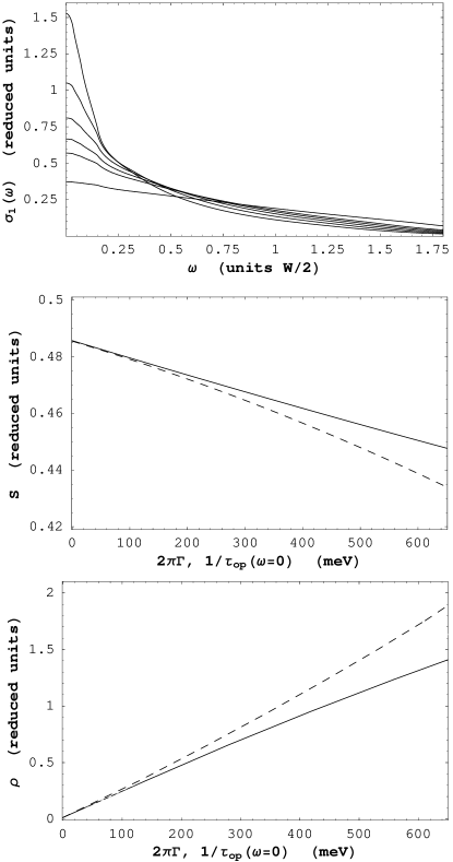
Figure 5: Top frame: real part of optical conductivity $\sigma_{1}(\omega)$ vs $\omega$ for $\Gamma=44,67,89,111,133,222$ meV (from top to bottom at $\omega=0$). Middle frame: dependence of the optical sum $S$ of Eq. (16) on $2\pi\Gamma$ (solid) and on $\tau^{-1}_{op}(\omega=0)$ (dashed). Bottom frame: dependencie of dc resistivity $\rho=1/\sigma_{1}(\omega=0)$ on $2\pi\Gamma$ (solid) and on $\tau^{-1}_{op}(\omega=0)$ (dashed). Dotted curve is the infinite band result. Temperature is $T=14.5$ K for all frames.

Six values of impurity parameters are used, namely $\Gamma=44.4,66.6,88.8,111.0,133.1,221.9$ meV. There are several features of these curves which are different from corresponding infinite band results. Perhaps the most obvious is that the total optical spectral weight $S$, defined in Eq. (16), is no longer independent of temperature and impurity content. [Temperature dependence is discussed in our previous paperknigavko04 .] The dependence of $S$ on $\Gamma$ is shown by the solid curve in the middle frame of Fig. 5. The optical spectral weight is measured in units $\pi e^{2}/[2Dm]$, such that in the infinite band case $S=1/2$. Because residual and inelastic scattering is no longer strictly additive in finite bands, the impurity parameter $\Gamma$ cannot be directly obtained from optical conductivity experiment. Therefore, we also plot $S$ vs $\tau^{-1}_{op}(\omega=0)$ (dashed curve), a parameter that is measurable. While there is a small difference between the two plots, both show that the total optical spectral weight is reduced as $\Gamma$ is increased. Another important property of the conductivity $\sigma_{1}(\omega)$ from Fig. 5, top frame, which needs to be commented upon, is its dc value, or its inverse $1/\sigma_{1}(\omega=0)$, the resistivity. This quantity is plotted in the bottom frame of Fig. 5 where it is seen to increase with $\Gamma$ (solid curve). This is also the case when plotted with respect to $\tau^{-1}_{op}(\omega=0)$ (dashed curve), and the dependence is not quite linear as would be expected in an infinite band (dotted line).

The behavior of solid curve can be understood from the formula for the resistivity: $\rho(T)=[\pi/(2S)]\tau^{-1}_{op}(\omega=0)$. While, as we have seen in a previous section, the approximate analytic formulas that can be obtained for the optical quantities, are not as accurate as for the self energy nevertheless they can be quite helpful in providing insight into the complete numerical results. Sharapov and Carbotte sharapov05 give the following expressions for inelastic and impurity contributions, respectively:

$${\tau_{op,{\rm phon}}^{-1}(\omega\rightarrow 0)} = 4\pi\int_{0}^{\infty}d\Omega\alpha^{2}F(\Omega)\int_{-\infty}^{+\infty}d\epsilon\frac{N(\epsilon)}{N_{0}(0)}[n(\Omega)+f(\Omega-\epsilon)]\left(-\frac{\partial f(\epsilon)}{\partial\epsilon}\right),$$ (35)

$${\tau_{op,{\rm imp}}^{-1}(\omega\rightarrow 0)} = 2\pi\Gamma\int_{-\infty}^{+\infty}d\epsilon\frac{N(\epsilon)}{N_{0}(0)}\left(-\frac{\partial f(\epsilon)}{\partial\epsilon}\right).$$ (36)

Besides the explicit thermal factor appearing in these equations, the temperature also enters through the renormalized DOS factor $N(\epsilon)$ which also depends on the phonon $\alpha^{2}F(\Omega)$ and on $\Gamma$ in contrast to the infinite band case. Independent of the details, because the $N(\epsilon)$ factor is everywhere smaller than its infinite band value of one, the resistivity is always reduced below its infinite band value. This reduction increase with increasing value of $\Gamma$ as we see in lower frame of Fig. 5 and is also increased with increasing temperature. At low temperatures the appropriate measure of the decrease in the impurity term of Eq. (36) is the value of $N(0)$ while for the inelastic term it depends on $N(\Omega)$ with $\Omega$ within the phonon range.

IV Very narrow bands

The case considered so far corresponds to a rather broad band as compared with the phonon energy. Nevertheless we found important qualitative changes from the infinite band case. Band structure calculationssatpathy92 for $K_{3}C_{60}$, as an example, give a half band width of about $250$ meV which is now comparable to the energy of the maximum phonon energy of $190$ meV in our model electron–phonon spectral density. For such cases Kostur and Mitrović kostur93 and later Pietronero, Strässler and Grimaldi pietronero95 have considered the effect of vertex corrections and a generalization of the Eliashberg equations which go beyond the Midgal theorem. The specific case of the Pauli susceptibility was considered by Cappelluti, Grimaldi and Pietronero cappelluti01 . In more recent work, Cappelluti and Pietronero cappelluti03 recognized that it was the effect of a finite band that primarily accounted for some of the qualitative differences found in their previous work and proceeded to include only these as a first step in understanding self energy renormalization. Here we follow their lead, but consider instead optical properties.

In this section we wish to accomplish three goals. First, we want to understand differences that arise when very narrow bands are involved as compared with relatively wide ones. Second, we want to compare a case with a larger value of $\lambda$ and finally we replace the three delta function model for $\alpha^{2}F(\omega)$ with a more realistic extended spectrum. We consider a model with three truncated Lorentzians:

$$\alpha^{2}F(\omega)=R(\lambda)\sum_{i=1}^{3}\frac{1}{2\pi}\left[\frac{\delta_{i}}{(\omega-\omega_{i})^{2}+\delta_{1}^{2}}-\frac{\delta_{i}}{\eta_{i}^{2}+\delta_{i}^{2}}\right]\Theta\left(\eta_{i}-\left|\omega-\omega_{i}\right|\right),$$ (37)

where $\omega_{i}$, the centers of the peaks, are the same as in Eq. (25). For each peak the parameter $\delta_{i}$ controls the half width, while the full spread is equal to $2\eta_{i}.$ The rescaling factor $R(\lambda)$ is inserted to guarantee a chosen value of $\lambda.$ Truncated Lorentzians are often used in the literature to introduce a smearing of the simple Einstein mode spectrum. For our numerical work we picked $\delta_{i}=0.2\omega_{i}$ and $\eta_{i}=0.6\omega_{i}$. In this case the peaks are wide and overlapping. The spectrum of Eq. (37) has the characteristic logarithmic mars-book frequency of $\omega_{ln}=96$ meV.

While, to set the parameters used here, we consider what might be reasonable for $K_{3}C_{60}$, i. e. we chose $W/2=250$ meV and an effective $\lambda$ of about one, we do not imply that our calculations can be applied directly to this specific system. Other complications such as the effect of Coulomb interactions yoo00 may need to be included as well. For example the small Drude peak seen in the experiments of Degiorgi et al degiorgi94 ; degiorgi95 which has a width of about $10-20$ meV and a weight representing only about $10-20$% of the total spectral weight is not understood in our work. On the other hand qualitative features of the memory function vs frequency dependence, such as the observed zero in its real part, are captured.

Figure 6: Frequency dependence of the renormalized density of states $N(\omega)/N_{0}$ for a very narrow band with $W/2=250$ meV (thin curves) with the parameters described in detail in the text. The heavy curve refers to $N(\omega)/N_{0}$ with $W/2=1.25$ eV for comparison.

In Fig. 6 we present a series of results for the dressed quasiparticle density of states $N(\omega)/N_{0}$ as a function of energy $\omega$. The heavy solid curve shows previous results for a rather wide band $W/2=1.25$ eV on a broader scale for the three delta function model of Eq. (25) with $\lambda=0.71$ and $\Gamma=22$ meV at low temperature $T=1.25$ K. It is to be compared with the other curves all of which are for a band that is five times narrower, namely $W/2=250$ meV. While for the wider band significant phonon structures are limited to an energy region well below the bare band cutoff at $\omega/(W/2)=1$, for the narrower band they dominate the shape of $N(\omega)/N_{0}$ even beyond $\omega/(W/2)=2$. No particular signature associated with the bare band edge remains. This is distinct from the heavy continuous curve which shows a smooth drop off at a new easily distinguishable renormalized band edge energy increased somewhat over its bare value and smeared by the interactions.

All thin solid curves in Fig. 6 are for the three delta function model of $\alpha^{2}F(\omega)$ with $\lambda=0.71$ at low temperature ($T=1.25$ K). The impurity parameter is $\Gamma=4.4,13.3$ and $39.9$ meV (from top to bottom). The dashed curve correspond to the extended spectrum of Eq. (37) with $\lambda=0.71$ and $\gamma=5$ meV at low temperature ($T=2.15$ K). The two sharp step like drops at $\omega/(W/2)<0.40$ present in the delta function case are now almost completely smeared out. The sharp spike like minimum at the energy of the maximum phonon energy $\omega/(W/2)=0.76$ [$\omega=190$ meV] and the near vertical drop at twice this energy, seen in the solid curves are gone in the dashed curve as are the distinct multiphonon structure at higher energies. The plateau like region at $0.8<\omega/(W/2)<1.3$ [for $\omega$ between $190$ and $390$ meV] in the solid curves becomes a shoulder in the dashed curve.

The modification of the renormalized density of states depends on the mass renormalization parameter $\lambda$. To demonstrate this we present in Fig. 6 the result for the same extended spectrum of Eq. (37)) and the same impurity parameter $\Gamma=4.4$ meV but with $\lambda=2$ (the dotted curve). Now the low temperature step at $\omega/(W/2)=0.16$ becomes visible and a deep and wide minimum develops in the frequency region of the most strongly coupled part of the electron–phonon spectral density centered at $\omega/(W/2)=0.76$. Additionally, the multiphonon processes become stronger, which is manifested by appearance of the maximum at $\omega/(W/2)\approx 1.4$ in the dotted curve in place of the shoulder in the dashed curve. Finally, the renormalized band edge has been shifted to much higher frequency and is not visible in Fig. 6.

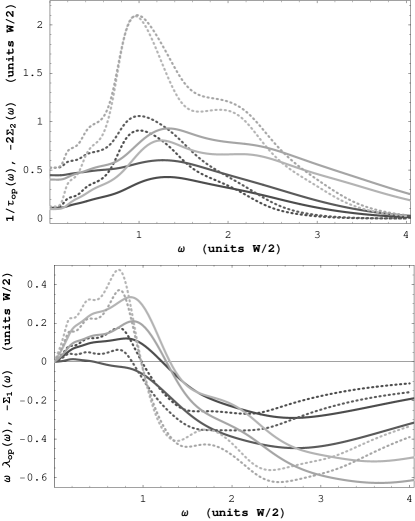
Figure 7: Top panel: Comparison of optical (solid curves) and quasiparticle (dotted curves) scattering rates. Bottom panel: Comparison of minus the real part of the self energy (dotted) with the corresponding optical quantity $\omega\lambda_{op}(\omega)$ (solid). The mass renormalization is $\lambda=2.0$ (grey curves) and $\lambda=0.71$ (black curves). In all cases there are two sets of curves corresponding to impurity parameter $\Gamma=5$ and $25$ meV. The extended $\alpha^{2}F(\Omega)$ of Eq. (37) was used. The half band width $W/2=250$ meV, temperature $T=2.15$ K.

Returning to the light continuous curves we note that, compared to the wide band case of the previous section, the phonon steps are now significantly reduced in magnitude as the impurity scattering is increased. For example, compare the bottom curve for $\Gamma=39.9$ meV to the top one for $\Gamma=4.4$ meV. These reductions go beyond non selfconsistent approximation and demonstrate that the selfconsistency becomes more important as the bare band width is reduced. The near additivity of electron–phonon and impurity contributions is lost. While for the curve corresponding to the purest case, the non self consistent approximation predicts well the size of the first step, it is not as good for the second and the third step is quite off. This is expected as in this case we are already not so far from the bare band edge and the selfconsistency becomes essential.

Note that at $\omega=0$ for the bottom light solid line with $\Gamma=39.9$ meV, $N(0)/N_{0}\approx 0.77$ in the numerical works. The non selfconsistent estimate $(1-2\Gamma/(W/2))\approx 0.68$ which is considerable smaller. However self consistency has actually reduced the impurity scattering rate below its infinite band value of $2\pi\Gamma$ because it is equal to $2\pi\Gamma N(0)$ and $N(0)/N_{0}(0)$ is smaller than one. Accounting for its 23% reduction eliminates much of the difference described above. A similar semiquantitative argument can be made to understand the reduction in phonon step size as $\Gamma$ increases when the simple non selfconsistent estimate begin to fail. Finally, we note the crossing of the light solid curves around $\omega/(W/2)\approx 0.8$ and the increase in density of states in the tails beyond $\omega/(W/2)=1.5$ as the impurity scattering is increased.

In Fig. 7 we turn to the memory function (solid lines) which is compared with the quasiparticle self energy (dotted lines) for several cases. We present results for $\lambda=0.71$ (black curves) and for $\lambda=2.0$ (grey curves) and for two different impurity content, $\Gamma=5$ and $25$ meV calculated with the model of the extended $\alpha^{2}F(\Omega)$ of Eq. (37). As expected both quasiparticle and optical scattering rates rise to a higher maximum value when $\lambda$ is larger, but the increase is not linear. This is followed by a drop towards zero as $\omega$ gets large instead of saturating at a common value of $2\pi a+2\pi\Gamma$ as discussed previously. The intercept of $\tau^{-1}_{op}(\omega)$ and $\tau^{-1}_{qp}(\omega)$ at $\omega=0$ is related to the elastic impurity scattering as the temperature for the figure is small $T=2.15$ K. For $\tau^{-1}_{qp}$ it does not depend on the value of $\lambda$ but for $\tau^{-1}_{op}$ it does. This can be seen most clearly in the top set of curves for which $\Gamma=25$ meV but is noticeable in the lower set with $\Gamma=5$ meV. When $\lambda$ is larger $\tau^{-1}_{op}$ at $\omega=0$ is smaller. This effect results from the Kubo formula and is not captured in any of our approximate analytic formulas. As previously noted $\tau^{-1}_{op}(\omega=0)<\tau^{-1}_{qp}(\omega=0)<2\pi\Gamma$.

For $\lambda=2$ the maximum value of $\tau^{-1}_{qp}(\omega)$ (see grey dotted curves in the top panel of Fig. 7) occurs at a frequency slightly below $\omega/(W/2)=1$ and is almost the same for the $\Gamma=5$ meV and $\Gamma=25$ meV. Although we have increased the impurity scattering we have not gained in maximum quasiparticle scattering. In an infinite band it would have risen from 3.22 to 3.72 for the parameters used. This effect is due to the self consistency. Both elastic and inelastic scattering involve not just $\alpha^{2}F(\Omega)$ and $\Gamma$ respectively but also the self consistent value of the dressed quasiparticle density of states $N(\omega)/N_{0}$ which becomes reduced as $\Gamma$ is increased. This in turn reduces both elastic and inelastic scattering rates leading, in case considered, to a saturation of the maximum in $\tau^{-1}_{qp}(\omega)$. For $\Gamma=5$ meV the rate is about 34% lower than its infinite band value and for $\Gamma=25$ meV it is about 43% lower. A similar situation holds for the case when $\lambda=0.71$ (black dotted curves) although in that case the maximum quasiparticle scattering does increase slightly with increasing $\Gamma$, for $\Gamma=5$ meV it is 26% below its infinite band value and for $\Gamma=25$ meV it is 40% below. Turning next to the optical scattering rate (solid curves in Fig. 7, top frame), we note first that they peaks at a higher frequency than does the corresponding quasiparticle rates. Also they are considerably smaller in magnitude, approximately 0.95 and 0.8 for $\Gamma=25$ and $5$ meV respectively for the case $\lambda=2$.

In the bottom frame of Fig. 7 we compare our results for the minus real part of the electronic self energy $-\Sigma_{1}(\omega)$ (dotted curves) with the corresponding optical quantity $\omega\lambda_{op}(\omega)$ (solid curves) of Eq. (18), which is the minus of the imaginary part of the memory function $M(\omega)$ defined in Eq. (15). It is quite clear that the optical masses (slopes at $\omega=0$ for solid curves) are in all cases considerably smaller than the quasiparticle masses (slopes at $\omega=0$ for dotted curves). As an example, for $\lambda=2$ the quasiparticle mass at $\Gamma=5$ meV is 1.1 as compared to 0.70 for the optical mass, while at $\Gamma=25$ meV we have 0.75 and 0.35 respectively. Using the non self consistent formula Eq. (28) gives for both masses $\lambda=2$ ($\lambda=0.71$) 1.1 (0.39) and 0.94 (0.21) for $\Gamma=5$ meV and $\Gamma=25$ meV respectively. For the pure case the agreement for the quasiparticle mass is good but this is no longer the case for $\Gamma=25$ meV. Also for the purer case considered on Fig. 7 the zero crossing of quasiparticle and optical mass renormalization function can be understood qualitatively with Eqs. (12) and (23) but these simple estimates begin to fail for higher values of $\Gamma$.

Finally, we comment on the reflectivity data of Degiorgi et al degiorgi94 ; degiorgi95 on $K_{3}C_{60}$. They did not analyze their data to extract optical scattering rate $\tau^{-1}_{op}(\omega)$ amd mass renormalization $\omega\lambda_{op}(\omega)$. Nevertheless we infer from the data presented three qualitative features. The value of $\tau^{-1}_{op}(\omega)$ at $\omega=0$ which gives a measure of the residual scattering is of order 160 meV. This large value is incompatible with the observed small Drude peak in $\sigma_{1}(\omega)$ of width 20 meV which contains about 12 % of the total optical spectral weight. Second, at $\omega\simeq 500$ meV the scattering rate has increased to approximately 500 meV which implies an inelastic contribution of 360 meV. Such a rise is much larger than can be achieved in the model of Fig. 6 and would indicate that the bare band width is somewhat larger than present band structure calculations predict and that the spectral $\lambda$ defined by the input electron–phonon spectral function $\alpha^{2}F(\omega)$ is even larger than 2. Thirdly, $\omega\lambda_{op}(\omega)$ changes sign at approximately 220 meV after which it plunges towards large negative values. This feature can be taken as the hallmark of finite band effects as it does not occur in infinite band theories. While such a zero crossing occurs naturally in our calculations and is generic, it is not clear that a set of microscopic parameters chosen to reproduce the features of the scattering rate $\tau^{-1}_{op}(\omega)$ would also accurately produce the position of the zero in the optical mass. We did not attempt such a combined fit as it would require a value of $\lambda$ which appears to be rather large.

V Conclusions

In an electronic system with a constant bare electronic density of states $N_{0}$ the application of a finite band cut off profoundly modifies the electron–phonon renormalization effects. In the infinite band case the dressed quasiparticle density of states $N(\omega)$ remains equal to $N_{0}$ and is independent of impurity scattering and temperature. A self consistent solution for the self energy in a finite band shows that $N(\omega)$ acquires low energy structure on the scale of the phonon energies. The band edge becomes smeared and the band extends beyond the original bare cut off. This extension of the band to higher energies is accompanied by a compensating reduction of spectral weight below the bare cut off. Equally importantly $N(\omega)$ is affected by impurity scattering and by temperature. $N(\omega=0)$ is reduced in both cases. On the other hand, while temperature rapidly smears out the phonon structure, impurities mainly reduce its amplitude.

The emphasis of previous works was on the effects of temperature and impurity scattering on the electron self energy $\Sigma(\omega)$, which is the quantity that determines quasiparticle properties. Here we have extended these works to optical properties and considered characteristic features of the memory function. For the infinite band case elastic impurity scattering just adds a constant amount ($2\pi\Gamma$) to the quasiparticle inelastic scattering rate, but in our case, because of the application of self consistency, they no longer add. Even at $\omega=0$ we find that $\tau^{-1}_{op}<\tau^{-1}_{qp}<2\pi\Gamma$. The well known result that, at high energies both optical and quasiparticle scattering rates due to phonons become equal and saturate at a value $2\pi a$ (with $a$ the area under the electron–phonon spectral density) no longer holds. While the maximum in $\tau^{-1}_{qp}$ can come close in value to $2\pi a+2\pi\Gamma$, the corresponding optical quantity $\tau^{-1}_{op}$ is much smaller in magnitude. Its maximum value increases with increasing $a$ but this increase is sublinear. A similar situation holds when $\Gamma$ is increased. At yet higher energies both scattering rates go to zero because of the finite band.

The known result that the real part of the quasiparticle self energy is unaffected by the impurity scattering no longer holds and this has an impact as well on the optical mass renormalization. Quasiparticle and optical effective mass renormalization at $\omega=0$ now differ from each other, neither is equal to $\lambda$ and both depend on impurity scattering. The real part of the self energy changes sign with increasing energy as does $\omega\lambda_{op}(\omega)$. The energy at which the zero crossing occurs is set by the phonon energy scale and can depend both on temperature and impurity content. It is larger for optics than it is for the self energy in many cases but not always. The optical spectral weight, i. e. the area under the absorptive part of the optical conductivity varies with temperature and with impurity scattering. The elastic and inelastic contributions to dc resistivity are no longer additive.

All these effects were found to be significant in magnitude even when a rather modest value of mass enhancement parameter $\lambda=0.71$ is used with a band width of 2.5 eV. While a three delta function $\alpha^{2}F(\omega)$ was used to emphasize boson structure with maximum phonon energy of 190 meV, a broader spectrum was also considered. This soften phonon structures but did not eliminate them. Of course, for simple metals such as Pb, the band width is much wider than considered above and the maximum phonon energy is also an order of magnitude smaller, so that in this case the infinite band approximation is appropriate and the finite band corrections found in this paper would be negligible. We have found that increasing the value of $\lambda$ to 2 increases boson structure but the increase is not linear in the value of $\lambda$. Also decreasing the value of W to 500 meV, a value suggested by band structure calculations in the alkali doped C₆₀, leads to a new regime in which important modifications due to the electron–phonon interaction dominate at all energies and no easily identifiable trace of the underlying bare electronic band cutoff remains.

While all these conclusions are based on numerical solution of the selfconsistent equations for the self energy and the Kubo formula for the conductivity, we have also derived more transparent analytical formulas evaluated in a non selfconsistent approximation. These simple formulas are not always accurate but give considerable insight into complete numerical results obtained and prove valuable in the analysis of optical data in finite band metals.

VI Acknowlegements

It is a pleasure to acknowledge useful discussions with J. Hwang, F. Marsiglio, B. Mitrović and S.G. Sharapov. Work supported by the Natural Science and Engineering Research Council of Canada (NSERC) and the Canadian Institute for Advanced Research (CIAR).

References

- (1) F. Marsiglio and J.P. Carbotte, in The Physics of Superconductivity, Vol. I: Conventional and High Tc Superconductors, edited by K.H. Bennemann and J.B. Ketterson (Springer Verlag, Berlin, 2003), p. 233.
- (2) B. Mitrović and J.P. Carbotte, Can. Jour. Phys. 61, 758 (1983); Can. Jour. Phys. 61, 784 (1983); Can. Jour. Phys. 61, 872 (1983).
- (3) W.E. Pickett, Phys. Rev. B 26, 1186 (1982).
- (4) B. Mitrović, Ph. D. Thesis, McMaster Univ. (1981).
- (5) E. Cappelluti and L. Pietronero, Phys. Rev. B 68, 224511, (2003).
- (6) F. Doğan and F. Marsiglio, Phys. Rev. B 68, 165102, (2003).
- (7) A. Knigavko and J.P. Carbotte, Phys. Rev. B 72, 035125, (2005).
- (8) A. Knigavko, J.P. Carbotte, and F. Marsiglio, Europhys. Lett. 71, 776, (2005).
- (9) M.P. Gelfand, Supercond. Review 1, 103 (1994).
- (10) S. Englesberg and J.R. Schrieffer, Phys. Rev. 131 993 (1963).
- (11) A.I. Liechtenstein, O. Gunnarsson, M. Knupfer, J. Fink, and J.F. Armbruster, J. Phys.: Condens. Matter 8, 4001 (1996).
- (12) F. Marsiglio, M. Schossmann, and J.P. Carbotte, Phys. Rev. B 37, 4965 (1988).
- (13) A. Chainani, T. Yokoya, T. Kiss, and S. Shin, Phys. Rev. Lett. 85, 1966 (2000).
- (14) F. Reinert, G. Nicolay, B. Eltner, D. Ehm, S. Schmidt, S. Hufner, U. Probst, and E. Bucher, Phys. Rev. Lett. 85, 3930 (2000).
- (15) F. Reinert, B. Eltner, G. Nicolay, D. Ehm, S. Schmidt, and S. Hufner, Phys. Rev. Lett. 91, 186406 (2003).
- (16) S.V. Shulga, O.V. Dolgov and E.G. Maksimov, Physica C, 178, 266 (1991).
- (17) J.W. Allen and J.C Mikkelsen, Phys. Rev. B 15, 2952 (1977).
- (18) A. V. Puchkov, D. N. Basov, and T. Timusk, J. Phys.: Condens. Matter 8, 10049 (1996).
- (19) F. Marsiglio and J. P. Carbotte, Aust. J. Phys. 50, 975 (1997).
- (20) M. A. Quijada, D. B. Tanner, R. J. Kelley, M. Onellion, H. Berger, and G. Margaritondo, Phys. Rev. B 60, 14917 (1999).
- (21) P.B. Allen, cond-mat/0407777.
- (22) F. Marsiglio and J.E. Hirsch, Physica C 165, 71 (1990).
- (23) P.B. Allen, Phys. Rev. B 3, 305 (1971).
- (24) S.V. Shulga, O.V. Dolgov, and E.G. Maksimov, Physica C 178, 266 (1991).
- (25) B. Mitrović and M.A. Fiorucci, Phys. Rev. B 31, 2694 (1985).
- (26) B. Mitrović and S. Perkowitz, Phys. Rev. B 30, 6749 (1984).
- (27) S.G. Sharapov and J.P.Carbotte, Phys. Rev. B, 72, 134506 (2005).
- (28) H.-Y. Choi, Phys. Rev. Lett. 81, 441 (1998).
- (29) J. Hwang, J. Yang, T. Timusk, S.G. Sharapov, J.P. Carbotte, D.A. Bonn, R. Liang, and W.N. Hardy, cond-mat/0505302.
- (30) S.V. Dordevic, C.C. Homes, J.J. Tu, T. Valla, M. Strongin, P.D. Johnson, G.D. Gu, and D.N. Basov, Phys. Rev. B71, 104529 (2005).
- (31) J.P. Carbotte, E. Schachinger, and J. Hwang, Phys. Rev. B71, 054506 (2005).
- (32) E. Schachinger, J.J. Tu, and J.P. Carbotte, Phys. Rev. B67, 214508 (2003).
- (33) J. Hwang, T. Timusk, and G.D. Gu, Nature (London) 427, 714 (2004) and private communication.
- (34) R.S. Markiewicz, S. Sahrakorpi, M. Lindroos, H. Lin, and A. Bansil, cond-mat/0503064.
- (35) E. Schachinger and J.P. Carbotte, Phys. Rev. B57, 13773 (1998); Phys. Rev. B64, 094501 (2002).
- (36) A. Knigavko, J.P. Carbotte and F. Marsiglio, Phys. Rev. B 70, 224501 (2004).
- (37) S. Satpathy, V.P. Antropov, O.K. Andersen, O. Jepsen, O. Gunnarsson, and A.I. Liechtenstein, Phys. Rev. B 46, 1773 (1992).
- (38) V.N. Kostur and B. Mitrović, Phys. Rev. B 48, 16388 (1993).
- (39) L. Pietronero, S. Strässler, and C. Grimaldi, Phys. Rev. B 52, 10516 (1995); C. Grimaldi, L. Pietronero, and S. Strässler, Phys. Rev. B 52, 10530 (1995).
- (40) E. Cappelluti, C. Grimaldi, and L. Pietronero, Phys. Rev. B 64, 125104 (2001).
- (41) J.-W. Yoo and H.-Y. Choi, Phys. Rev. B 62, 4440 (2000).
- (42) L. Degiorgi, E.J. Nicol, O. Klein, G. Grüner, P. Wachter, S.-M. Huang, J. Wiley, and R.B. Kaner, Phys. Rev. B 49, 7012 (1994).
- (43) L. Degiorgi, Mod. Phys. Lett. B9, 8445 (1995).