Distinguishing Patterns of Charge Order: Stripes or Checkerboards

Abstract

In two dimensions, quenched disorder always rounds transitions involving the breaking of spatial symmetries so, in practice, it can often be difficult to infer what form the symmetry breaking would take in the “ideal,” zero disorder limit. We discuss methods of data analysis which can be useful for making such inferences, and apply them to the problem of determining whether the preferred order in the cuprates is “stripes” or “checkerboards.” In many cases we show that the experiments clearly indicate stripe order, while in others (where the observed correlation length is short), the answer is presently uncertain.

I Introduction

Charge ordered states are common in strongly correlated materials, including especially the cuprate high temperature superconductors. Identifying where such phases occur in the phase diagram, and where they occur as significant fluctuating orders is a critical step in understanding what role they play in the physics, more generally. Since “charge ordered” refers to states which spontaneously break the spatial symmetries of the host crystal, identifying them would seem to be straightforward. However, two real-world issues make this less simple than it would seem. In the first place, quenched disorder (alas, an unavoidable presence in real materials), in all but a very few special circumstances, rounds the transition and spoils any sharp distinction between the symmetric and broken symmetry states. Moreover, the charge modulations involved tend to be rather small in magnitude, and so difficult to detect directly in the obvious experiments, such as X-ray scattering.

In a previous paper, Kivelson et al. (2003) three of us addressed at some length the issue of how the presence or absence of charge order or incipient charge order can best be established in experiment. In the present paper we focus on a related issue: in a system in which charge order is believed to exist, how can the precise character of the charge order best be established? This is particularly timely given the spectacular developments in scanning tunneling microscopy (STM) which produces extremely evocative atomic scale “pictures” of the local electronic structure – the question is how to extract unambiguous conclusions from the cornucopia Hoffman et al. (2002a, b); Howald et al. (2003a, b); McElroy et al. (2003, 2005); Momono et al. (2005); Hanaguri et al. (2004) of data. We take as a representative example, the issue of whether the charge order that is widely observed in the cuprates is “stripes” (which in addition to breaking the translation symmetry, breaks various mirror and discrete rotation symmetries of the crystal) or “checkerboards” (an order which preserves the point-group symmetries of the crystal). To address this issue, we generate simulated STM data and then test the utility of various measures we have developed for discriminating different types of order by applying them to this simulated data. Where the correlation length for the charge order is long, definitive conclusions can be drawn relatively simply - consequently, it is possible to conclude that the preferred charge order in the 214 (La₂CuO₄) family of materials is stripes and not checkerboards.Tranquada et al. (1995) However, where the correlation length is short (disorder effects are strong), it turns out (unsurprisingly) to be very difficult to develop any fool-proof way to tell whether the observed short-range order comes from pinned stripes or pinned checkerboards – for example, the image in Fig. 1 (right panel) corresponds to disorder-pinned stripes, despite the fact that, to the eye, the pattern is more suggestive of checkerboard order (with the latter seen in Fig. 2 (right panel)).

In Section II, we give precise meaning in terms of broken symmetries to various colloquially used descriptive terms such as “stripes,” “checkerboards,” “commensurate,” “incommensurate,” “diagonal,” “vertical,” “bond-centered,” and “site-centered.” In Section III we write an explicit Landau-Ginzburg (LG) free energy functional for stripe and checkerboard orders, including the interactions between the charge order and impurities. In Section IV we generate simulated STM data by minimizing the LG free energy in the presence of disorder. (See Figs. 1 and 2.) The idea is to develop strategies for solving the inverse problem: Given the simulated data, how do we determine whether the “ideal” system, in the absence of disorder, would be stripe or checkerboard ordered, and indeed, whether it would be ordered at all or merely in a fluctuating phase with a large CDW susceptibility reflecting the proximity of an ordered state. In Section IV, we define several quantitative indicators of orientational order that are useful in this regard, but unless the correlation length is well in excess of the CDW period, no strategy we have found allows confident conclusions. In Section V, we show that the response of the CDW order parameter to various small symmetry breaking fields, such as a small orthorhombic distortion of the host crystal, can be used to distinguish different forms of charge order. In Section VI, we apply our quantitative indicators to a sample of STM data in Bi₂Sr₂CaCu₂O_8+δ and discuss the results. In Section VII we conclude with a few general observations.

II General Considerations

Stripes are a form of unidirectional charge order (see Fig. 1 (left panel), characterized by modulations of the charge density at a single ordering vector, $\bf Q$, and its harmonics, ${\bf Q}_{n}=n\bf Q$ with $n=$ an integer. In a crystal, we can distinguish different stripe states not only by the magnitude of $\bf Q$, but also by whether the order is commensurate (when $|{\bf Q}|a=2\pi(m/n)$ where $a$ is a lattice constant and $n$ is the order of the commensurability) or incommensurate with the underlying crystal, and on the basis of whether $\bf Q$ lies along a symmetry axis or not. In the cuprates, stripes that lie along or nearly along the Cu-O bond direction are called “vertical” and those at roughly $45^{\circ}$ to this axis are called “diagonal.” In the case of commensurate order, stripes can also be classified by differing patterns of point-group symmetry breaking - for instance, the precise meaning of the often made distinction between so-called “bond-centered” and “site-centered” stripes is that they each leave different reflection planes of the underlying crystal unbroken. Furthermore, it has been argued that bond and site-centered stripes may be found in the same material, Li et al. (2003) and even may coexist at the same temperature.Wochner et al. (1998) The distinction between bond and site-centered does not exist for incommensurate stripes. If the stripes are commensurate, then $\bf Q$ must lie along a symmetry direction, while if the CDW is incommensurate, it sometimes will not.

Checkerboards are a form of charge order (see Fig. 2 (left panel) that is characterized by bi-directional charge density modulations, with a pair of ordering vectors, $\mathbf{Q}_{1}$ and $\mathbf{Q}_{2}$ (where typically $\left|\mathbf{Q}_{1}\right|=\left|\mathbf{Q}_{2}\right|$.) Checkerboard order generally preserves the point group symmetry of the underlying crystal if both ordering vectors lie along the crystal axes. In the case in which they do not, the order is rhombohedral checkerboard and the point group symmetry is not preserved. As with stripe order, the wave vectors can be incommensurate or commensurate, and in the latter case $\mathbf{Q}_{j}\,a=2\pi\left(m/n,m^{\prime}/n^{\prime}\right)$. Commensurate order, as with stripes, can be site-centered or bond-centered.

III Landau-Ginzburg Effective Hamiltonian

To begin with, we will consider an idealized two dimensional model in which we ignore the coupling between layers and take the underlying crystal to have the symmetries of a square lattice. We further assume that in the possible ordered states, the CDW ordering vector lies along one of a pair of the orthogonal symmetry directions, which we will call “$x$” and “$y$”. We can thus describe the density variations in terms of two complex scalar order parameters,

$$\rho(\mathbf{r})=\bar{\rho}+[\varphi_{1}(\mathbf{r})e^{iQ_{x}x}+\varphi_{2}(\mathbf{r})e^{iQ_{y}y}+{\rm c.c.}]$$ (1)

(For simplicity, we will take $Q_{x}=Q_{y}$ throughout.) Note, the “density, ” in this case, can be taken to be any scalar quantity, for instance the local density of states, and need not mean, exclusively, the charge density.

To quartic order in these fields and lowest order in derivatives, and assuming that commensurability effects can be neglected, the most general Landau-Ginzburg effective Hamiltonian density consistent with symmetry has been written down by several authors: McMillan (1975); Nakanishi and Shiba (1975); Sachdev and Demler (2004); Zhang et al. (2002)

$$H_{eff}=\frac{\kappa_{L}}{2}\left[|\partial_{x}\varphi_{1}|^{2}+|\partial_{y}\varphi_{2}|^{2}\right]+\frac{\kappa_{T}}{2}\left[|\partial_{y}\varphi_{1}|^{2}+|\partial_{x}\varphi_{2}|^{2}\right]$$

$$+\frac{\alpha}{2}\left[|\varphi_{1}|^{2}+|\varphi_{2}|^{2}\right]+\frac{u}{4}\left[|\varphi_{1}|^{2}+|\varphi_{2}|^{2}\right]^{2}+\gamma|\varphi_{1}|^{2}|\varphi_{2}|^{2}$$

(2)

The sign of $\alpha$ determines whether one is in the broken symmetry phase ($\alpha<0$) or the symmetric phase ($\alpha>0$), and in the broken symmetry phase, $\gamma$ determines whether the preferred order is stripes ($\gamma>0$) or checkerboards ($\gamma<0$). Note that for stability, it is necessary that $\gamma>-u$ and $u>0$; if these conditions are violated, one needs to include higher order terms in $H_{eff}$. Without loss of generality, we can rescale distance so that $\kappa_{L}=1$ and the order parameter magnitude such that $u=1$. For simplicity, in the present paper, we will also set $\kappa_{L}=\kappa_{T}$, although the more general situations can be treated without difficulty. The phases of this model in the absence of disorder are summarized in Table 1.

	$\alpha>0$	$\alpha<0$
	Symmetric	Broken Symmetry
$\gamma>0$	$\genfrac{(}{)}{0.0pt}{}{{\rm Fluctuating}}{{\rm Stripes}}$	(Stripes)
	Symmetric	Broken Symmetry
$\gamma<0$	$\genfrac{(}{)}{0.0pt}{}{{\rm Fluctuating}}{{\rm Checkerboard}}$	(Checkerboard)

Table 1: Phases of the Landau-Ginzburg model, in the absence of disorder.

Imperfections of the host crystal enter the problem as a quenched potential, $U(\mathbf{r})$:

$$H_{dis}=U(\mathbf{r})\rho(\mathbf{r})$$ (3)

To be explicit, we will take a model of the disorder potential in which there is a concentration of impurities per unit area, $\delta/a^{2}$ where $a$ is the “range” of the impurity potential and $U_{0}$ is the impurity strength, so $U(\mathbf{r})=\sum_{i}U_{0}\Theta[a^{2}-(\mathbf{r}-\mathbf{r}_{i})^{2}]$, where the sum is over the (randomly distributed) impurity sites, $\mathbf{r}_{i}$ and $\Theta$ is the Heaviside function. We have arbitrarily taken $a$ to be 1/4 the period, $\lambda$, of the CDW, i.e. $\lambda\equiv 2\pi/|{\bf Q}|$ and $a=\lambda/4$. (This choice is motivated by the fact that, in many cases, the observed charge order has a period $\lambda\approx 4$ lattice constants.)

IV Analysis of the simulated data

In this section we will show how these ideas can be used to interpret STM images in terms of local stripe order. In Ref.[Kivelson et al., 2003] it was shown that local spectral properties of the electron Green function of a correlated electron system, integrated over an energy range over a window in the physically relevant low energy regime, can be used as a measure of the local order. This is so even in cases in which the system is in a phase without long range order but close enough to a quantum phase transition (“fluctuating order”) that local defects can induce local patches of static order. From this point of view any experimentally accessible probe with the correct symmetry can be used to construct an image of the local order state. In applying the following method to real experimental data, one must take as a working assumption that the image obtained is representative of some underlying order, be it long-ranged or incipient. This analysis, of course, would not make sense if the data is not, at least in substantial part, dominated by the correlations implied by the existence of an order parameter.

We generate simulated data as follows: For a given randomly chosen configuration of impurity sites, we minimize $H_{eff}+H_{dis}$ with respect to $\varphi$. This is done numerically using Newton’s method. The order parameter texture is then used to compute the resulting density map according to Eq. 1. This we then treat as if it were the result of a local imaging experiment, such as an STM experiment.

Even weak disorder has a profound effect on the results. For $\alpha<0$, collective pinning causes the broken symmetry state to break into domains with a characteristic size which diverges exponentially as $U_{0}\to 0$ (In three dimensions, the ordered state survives as long as the disorder is less than a critical value.) Examples of this are shown in Fig. 1 and Fig. 2, where data with a given configuration of impurities with concentration $\delta=0.1$ are shown for various strengths of the potential, $U_{0}$. For a checkerboard phase ($\gamma<0$), the domain structure is rather subtle, involving shifts of the phase of the density wave as a function of position as can be seen in Figs. 2(left and center panels).In the stripe phase, in addition to phase disorder, there is a disordering of the orientational (“electron nematic”) order, resulting in a more visually dramatic breakup into regions of vertical and horizontal stripes, as can be seen in Fig. 1 (center panel).

The effect of quenched disorder in the symmetric phase ($\alpha>0$) is somewhat different. In a sense, the effect of the disorder is to pin the fluctuating order of the proximate ordered phase. However, here, whether the disorder is weak or strong, it is nearly impossible to distinguish fluctuating stripes from checkerboards. Fig. 1 (right panel) and Fig. 2 (right panel) illustrate this phenomenon. This is easily understood in the weak disorder limit, where

$$\varphi_{j}(\mathbf{r})=\int d\mathbf{r}^{\prime}\chi_{0}(\mathbf{r}-\mathbf{r}^{\prime})e^{-i{\bf Q}\cdot\mathbf{r}^{\prime}}U(\mathbf{r}^{\prime})+{\cal O}(U^{3})$$ (4)

where the susceptibility,

$$\chi_{0}(\mathbf{r})=K_{0}(\sqrt{\alpha}\mathbf{r}),$$ (5)

is expressed in terms of the $K_{0}$ Bessel function and is independent of $\gamma$. Near criticality ($1\gg\alpha>0$), the susceptibility is very long ranged, so a significant degree of local order can be pinned by even a rather weak impurity potential. However, only the higher order terms contain any information at all about the sign of $\gamma$, and by the time they are important, the disorder is probably already so strong that it blurs the distinction between the two states, anyway.

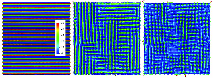
Figure 1: (color online) left panel: Highly stripe-ordered system, with weak impurities, $U_{0}=0.1$, $\delta=0.1$. Here $\gamma=1$, $\alpha=-0.05$. [Scale is arbitrary.] center panel: Otherwise identical to the first system (including the spatial distribution and concentration of impurities), but the strength each impurities has increased to $U_{0}=0.75$. right panel: Identical to the left panel, except $\alpha=+0.05$. Much of the underlying charge pattern remains, even to positive $\alpha$, where in the absence of impurities, the system would be homogeneous. All graphs are approximately 20 CDW wavelengths in width.

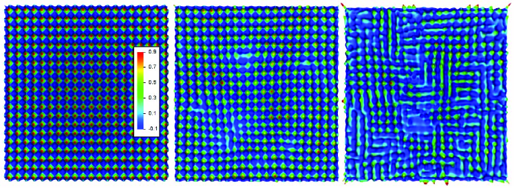
Figure 2: (color online) The parameters entering the effective Hamiltonian and the impurity realizations are identical here to the panels of Fig. 1, with the exception of the symmetry breaking term, $\gamma$, which is now $-0.95$. (In the center panel, because the checkerboard state is more stable than the analogous stripe state, we have taken $U_{0}=1.5$.) Unlike the stripe ordered system, the checkerboard system does not break into domains, but rather develops pair wise dislocations. In 2 (center panel), three pairs of such dislocations are visible. Note the similarity between the right panel of each set of Fig.1 and Fig.2; the sign of $\gamma$ has little effect for $\alpha>0$.

IV.1 Diagnostic Filters

Now, our task is to answer the question: Given a set of simulated data, what quantitative criteria best allows us to infer the form of the relevant correlations in the absence of disorder? For sufficiently weak disorder, these criteria are, at best, just a way of quantifying a conclusion that is already apparent from a visual analysis of the data. Where disorder is of moderate strength, such criteria may permit us to reach conclusions that are somewhat less prejudiced by our preconceived notions. Of course, when the disorder is sufficiently strong that the density-wave correlation length is comparable to the CDW period, it is unlikely that any method of analysis can yield a reliable answer to this question.

Firstly, to eliminate the rapid spatial oscillations, we define two scalar fields (which we will consider to be the two components of a vector field, $\bf{A}(\mathbf{r})$) corresponding to the components of the density which oscillate, respectively, with wave vectors near ${Q\hat{x}}$ and $Q\hat{y}$:

$${\rm A}_{j}(\mathbf{r})=\int\mbox{d}\mathbf{r}^{\prime}F_{j}(\mathbf{r}-\mathbf{r}^{\prime})\rho(\mathbf{r}^{\prime})$$ (6)

where we take $F_{j}$ to be the coherent state with spatial extent equal to the CDW period:

$$F_{j}(\mathbf{r})=\frac{Q^{2}}{2\pi^{2}}\exp[i\,Q_{j}r_{j}-r^{2}/(2\pi\lambda^{2})]$$ (7)

(no summation over $j$.)

In terms of ${\bf A}$ we construct three quantities which can be used in interpreting data:

$$\xi_{CDW}^{2} \equiv \frac{\left|\int\mbox{d}\mathbf{r}{\bf A}\right|^{2}}{\int\mbox{d}\mathbf{r}\left|\bf A\right|^{2}}$$ (8)

$$\xi_{orient}^{2} \equiv \frac{\left|\int\mbox{d}\mathbf{r}\left[\left|{\rm A}_{1}\right|^{2}-\left|{\rm A}_{2}\right|^{2}\right]\right|^{2}}{\int\mbox{d}\mathbf{r}\left|\left|{\rm A}_{1}\right|^{2}-\left|{\rm A}_{2}\right|^{2}\right|^{2}}$$ (9)

$$\eta_{orient} \equiv \frac{\int\mbox{d}\mathbf{r}\left|\left|{\rm A}_{1}\right|^{2}-\left|{\rm A}_{2}\right|^{2}\right|^{2}}{\int\mbox{d}\mathbf{r}\left|\left|{\rm A}_{1}\right|^{2}+\left|{\rm A}_{2}\right|^{2}\right|^{2}}$$ (10)

The quantities called $\xi$ have units of length and $\eta_{orient}$ is dimensionless. All of these quantities are invariant under a change of units, $\rho(\mathbf{r})\to\Lambda\rho(\mathbf{r})$; this is important since in many experiments, including STM, the absolute scale of the density oscillations is difficult to determine because of the presence of unknown matrix elements.

$\xi_{CDW}$ has the interpretation of a CDW correlation length. In the absence of quenched disorder, and for $\alpha<0$, $\xi_{CDW}\sim L$, where $L$ is the linear dimension of the sample. In the presence of disorder, $\xi_{CDW}$ is an average measure of the domain size. For $\alpha>0$ and weak but non-vanishing disorder, $\xi_{CDW}\sim\alpha^{-1/2}$, as can be seen from a scaling analysis of Eq. 4. The evolution of $\xi_{CDW}$ as a function of $\alpha$ is shown in Fig. 3 for a system of size $L=20\lambda$, for various strengths of the disorder and for stripes (Fig. 3 (top panel) and checkerboards (Fig. 3 (bottom panel).) $\xi_{CDW}$ is generally a decreasing function of increasing disorder, although for $\alpha>0$ there is a range in which it exhibits the opposite behavior. For fixed, non-zero disorder, we see that a large value of $\xi_{CDW}>4$ almost inevitably means that $\alpha<0$, i.e. that the density patterns are related to a domain structure of what would otherwise have been a fully ordered state. However, smaller values of $\xi_{CDW}$ can either come from weak pinning of CDW order which would otherwise be in a fluctuating phase, or a very small domain structure due to strong disorder.

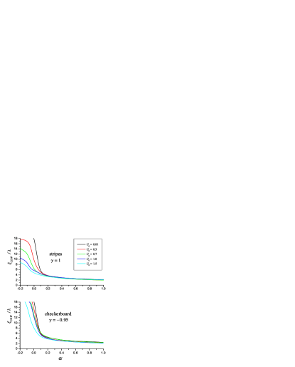
Figure 3: (color online) $\xi_{CDW}$ vs. $\alpha$ (measured in units of the CDW wavelength). top panel) $\gamma=1$, bottom panel) $\gamma=-0.95$. In a perfectly clean system, $\xi_{CDW}$ vanishes for $\alpha>0$, whereas with even a little disorder, charge order is induced. For $U_{0}>1$ and $\alpha<0$, disorder affects $\xi_{CDW}$ more strongly in the stripe system. For $\alpha>0$, there is little distinction in either the sign of $\gamma$ or the strength of $U_{0}$. All quantities in Figs. 3,4 and 5 are computed for systems of size $20\lambda\times 20\lambda$ and averaged over 50 or more realizations of the disorder.

The CDW correlation length does not distinguish between stripe and checkerboard patterns. However, for $\alpha<0$, the orientational amplitude $\eta_{orient}$ is an effective measure of stripiness. In the clean system with $\alpha<0$, $\eta_{orient}$ approaches unity for $\gamma>0$ and is zero for $\gamma<0$. While quenched disorder somewhat rounds the sharp transition in $\eta_{orient}$ at $\gamma=0$, it is clear from Fig. 4 (top panel) that values of $\eta_{orient}>0.2$ are clear indicators of stripe order, and $\eta_{orient}<0.2$ implies checkerboard. In the absence of disorder, $\eta_{orient}$ is ill-defined for $\alpha>0$, and even for non-zero disorder, the behavior of $\eta_{orient}$ is difficult to interpret in the fluctuating order regime, as is also clear from Fig. 4. The orientational correlation length, $\xi_{orient}$, gives similar information as $\eta_{orient}$, and suffers from the same shortcomings.

One interesting possibility is that, for a weakly disordered stripe phase, one can imagine an orientational glass in which $\xi_{orient}\gg\xi_{CDW}$, i.e. the CDW order is phase disordered on relatively short distances, but the orientational order is preserved to much longer distances. In Fig. 5, we plot the ratio of $\xi_{orient}/\xi_{CDW}$ for $\gamma=1$ (strong preference for stripes) as a function of $\alpha$ for various values of the disorder. Clearly, we have not found dramatic evidence of such an orientational glass, although we have not carried out an exhaustive search. Nonetheless, for $\alpha<0$, this ratio is manifestly another good way to distinguish stripe and checkerboard order.

The bottom line: If $\xi_{CDW}$ is a few periods or more, it is possible to conclude that $\alpha<0$, ı.e. that in the absence of impurities there would be long-range CDW order. If $\xi_{CDW}$ is shorter than this, then either the impurity potential is very strong (which should be detectable in other ways) or $\alpha\sim\xi_{CDW}^{-2}$ is positive. For intermediate values of $\xi_{CDW}$, all that can be inferred is that the system is near critical, $|\alpha|\ll 1$. Given a substantial $\xi_{CDW}$, it is possible to distinguish a pinned stripe phase from a pinned checkerboard phase for which $\eta_{orient}$ is greater than or less than 0.2, respectively.

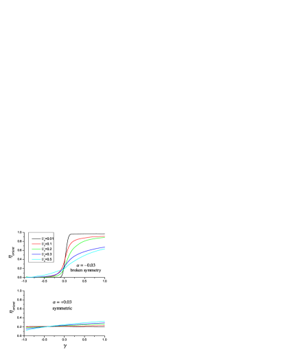
Figure 4: (color online) $\eta_{orient}$ vs. $\gamma$: top panel) $\alpha<0$. In the ordered phase, $\eta_{orient}$ is good indicator of the nature of the underlying order (i.e the sign of $\gamma$. At large $U_{0}$, the distinction is lost, and the result approaches that of the symmetric phase ($\alpha>0$), shown in the bottom panel. We observe that the nearly uniform value of $\eta_{orient}\approx 0.2$ in the $\alpha>0$ measurements intersects the (all of the) data in the ($\alpha=-0.03$) graph at the $\gamma=0$ axis.

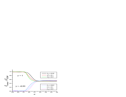
Figure 5: (color online) $\xi_{orient}/\xi_{CDW}$ vs. $\alpha$: For $\alpha<0$, $\xi_{orient}/\xi_{CDW}$ is a strong indicator of the sign of $\gamma$. For $\alpha>0$ and either sign of $\gamma$, the disorder-averaged ratio is $1/2$, largely independent of other parameters.

V Effect of an orthorhombic distortion

An orthorhombic distortion breaks the C₄ symmetry of the square lattice down to C₂. There are two distinct ways this can occur - either the square lattice can be distorted to form rectangles, as shown in Fig. 6a, in which case the “preferred” orthorhombic axis is either vertical or horizontal, or the squares can be distorted to form rhombi, as shown in Fig. 6b, in which case the preferred orthorhombic axis is diagonal. A general orthorhombic distortion is represented by a traceless symmetric tensor, $O_{ab}$; an orthorhombic distortion corresponding to Fig. 6b is represented by ${\bf O}=h{\bf\sigma}_{3}$ while Fig. 6b is ${\bf O}=h{\bf\sigma}_{1}$ where $h$ is the magnitude of the symmetry breaking and ${\bf\sigma}_{j}$ are the Pauli matrices. Then

$$H_{ortho}=-O_{ab}Q_{a}Q_{b}\left[|\varphi_{1}|^{2}-|\varphi_{2}|^{2}\right]\hskip 42.67912pt$$

$$+\ \ g\left[Q_{a}O_{ab}\varphi_{1}^{\star}\partial_{b}\varphi_{1}-\epsilon_{a\bar{a}}Q_{a}O_{\bar{a}b}\varphi_{2}^{\star}\partial_{b}\varphi_{2}\right]+\ldots$$ (11)

where $\ldots$ is higher order terms.

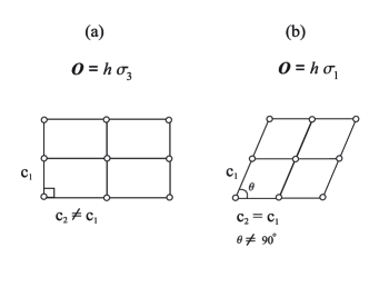
Figure 6: Orthorhombic symmetry breaking reduces a square lattice to a lower symmetry. (a) Rectangular lattice distortion (exaggerated). The preferred orthorhombic axis lies along an original lattice vector (i.e. along the lines connecting atomic sites.) (b) A rhombohedral distortion leaves the preferred orthorhombic axis diagonal to the original lattice vectors.

In case (a), the first term is non-zero, and hence dominant. For $h$ positive, this enhances $\varphi_{1}$ and suppresses $\varphi_{2}$. In a stripe phase, this has the same effect as a magnetic field in a ferromagnet - it chooses among the otherwise degenerate vertical and horizontal stripe ordered states, so one is preferred.Carlson et al. (2005) For checkerboard order, it produces a distortion of the fully ordered state, so that the expectation value of $\varphi_{1}$ exceeds the expectation value of $\varphi_{2}$. Moreover, it results in a split phase transition, so that as a function of decreasing temperature, rather than a single transition from a symmetric high temperature phase to a low temperature checkerboard phase, in the orthorhombic case there are two transitions, the first to a stripe ordered phase, and then at a temperature smaller by an amount proportional to $h$, a transition to a distorted checkerboard phase. The second term, proportional to $g$, is subdominant in this case, but still has a significant effect. For an incommensurate stripe phase, it results in a small shift in the ordering wave vector ${\bf Q}\to\tilde{\bf Q}={\bf Q}(1-gh/\kappa_{L})$. In an incommensurate checkerboard phase, it results in a relative shift of the two ordering vectors, ${\bf Q}\to\tilde{\bf Q}={\bf Q}(1-gh/\kappa_{L})$ and ${\bf Q}^{\prime}\to\tilde{\bf Q}^{\prime}={\bf Q}^{\prime}(1+gh/\kappa_{L})$ one toward smaller and the other toward larger magnitude producing a rectangular checkerboard. In the case in which the order is commensurate, it is locked to the lattice, and therefore the only shifts in ordering wave-vectors are proportional to the (usually miniscule) shifts of the lattice constant.

In case (b), the first term vanishes, so the second term is dominant. For incommensurate order, this results in a small rotation of the ordering vector away from the crystalline symmetry axis. To first order in $h$, the new ordering vector is $\tilde{\bf Q}=|{\bf Q}|\langle 1,k\rangle$ with $k=gh/\kappa_{T}$ and, in the case of checkerboard order, the second ordering vector is $\tilde{\bf Q}^{\prime}=|{\bf Q}|\langle k,1\rangle$. Again, in the commensurate case, the order remains locked to the lattice until the magnitude of the orthorhombicity exceeds a finite critical magnitude.

To summarize, the response of charge order to small amounts of orthorhombicity can be qualitatively different depending on whether the order is commensurate or incommensurate and checkerboard or striped.

V.0.1 More complex patterns of symmetry breaking

It is useful to point out that with complex crystal structures, the application of the above ideas requires some care. For example, there are some cuprate superconductors which exhibit a so called Low Temperature Tetragonal (LTT) phase. This phase has an effective orthorhombic distortion of each copper oxide plane, but has two planes per unit cell and a four-fold twist axis which is responsible for the fact that it is classified as tetragonal. In the first plane, ${\bf O}=h{\bf\sigma}_{3}$, and in the second ${\bf O}=-h{\bf\sigma}_{3}$. Note that this means that for stripe order, there will be four ordering vectors, a pair at $\tilde{\bf Q}=\pm|{\bf Q}|\langle 1+hg/\kappa_{L},0\rangle$ from the first plane and a pair at $\tilde{\bf Q}=\pm|{\bf Q}|\langle 0,1+hg/\kappa_{L}\rangle$ from the other. However, for incommensurate checkerboard order, there should be eight ordering vectors: $\pm|{\bf Q}|\langle 1+hg/\kappa_{L},0\rangle$, $\pm|{\bf Q}|\langle 1-hg/\kappa_{L},0\rangle$, $\pm|{\bf Q}|\langle 0,1+hg/\kappa_{L}\rangle$, and $\pm|{\bf Q}|\langle 0,1-hg/\kappa_{L}\rangle$.

VI Analysis of experiments in the cuprates

There have been an extremely large number of experiments which have been performed on various closely related cuprates, both superconducting and not, which have been interpreted as evidence for or against the presence of charge order of various types. For instance, there is a large amount of quasi-periodic structure observed in the local density of states measured by scanning tunneling microscopy (STM) on the surface of superconducting Bi₂Sr₂CaCu₂O_8+δ crystals, but there is controversy concerning how much of this structure arises from the interference patterns of well-defined quasiparticles whose dispersion is determined by the d-wave structure of the superconducting gap Hoffman et al. (2002a); McElroy et al. (2003); Wang and Lee (2003); Bena et al. (2004) and how much reflects the presence of charge order or incipient charge order.Howald et al. (2003a); Hoffman et al. (2002b); Howald et al. (2003b); McElroy et al. (2005); Momono et al. (2005); Kivelson et al. (2003) A similar debate has been carried out concerning the interpretation of the structures seen in inelastic neutron-scattering experiments.Tranquada (2005, 2004); Fujita et al. (2004); Li et al. (2003); Hinkov et al. (2004); Bourges et al. (2000); Mook et al. (2000); Christensen et al. (2004); Kivelson et al. (2003)

As mentioned in the introduction, the issue of how to distinguish charge order from interference patterns was discussed in detail in a recent review,Kivelson et al. (2003) and so will not be analyzed here. Here, we will accept as a working hypothesis the notion that various observed structures should be interpreted in terms of actual or incipient order, and focus on identifying the type of order involved.

VI.1 Neutron and X-ray scattering

Scattering experiments in several of the cuprates, most notably La_2-xSr_xCuO₄, La_1.6-xNd_0.4Sr_xCuO₄, La_2-xBa_xCuO₄, and O-doped La₂CuO₄ have produced clear and unambiguous evidence of charge and spin ordering phenomena with a characteristic ordering vector which changes with doping.Yamada et al. (1998); Cheong et al. (1991); Tranquada et al. (1995); Thurston et al. (1992); Mason et al. (1992); Yamada et al. (1997); Tranquada et al. (1996, 1997); Stock et al. (2002, 2004) The evidence is new peaks in the static structure factor corresponding to a spontaneous breaking of translational symmetry, leading to a new periodicity longer than the lattice constant of the host crystal. In many cases, the period is near 4 lattice constants for the charge modulations and 8 lattice constants for the spin. The peak-widths correspond to a correlation length Lee et al. (1999); Tranquada et al. (1997) that is often in excess of 20 periods. For technical reasons, the spin-peaks are easier to detect experimentally, but where both are seen, the charge ordering peaks are always seen Wochner et al. (1998); Abbamonte et al. (2005); v. Zimmermann et al. (1998); Fujita et al. (2002a); Reznik et al. (2005) to be aligned with the spin-ordering peaks, and the charge period is 1/2 the spin period.

Except in the case Wakimoto et al. (1999); Fujita et al. (2002b) of a very lightly doped ($x<0.05$) LSCO (where the stripes lie along an orthorhombic symmetry axis, so only two peaks are seen), there are four equivalent spin-ordering peaks and, where they have been detected, four equivalent charge ordering peaks. Thus, the issue arises whether this should be interpreted as the four peaks arising from some form of checkerboard order, or as two pairs of peaks arising from distinct domains of stripes - half the domains with the stripes oriented in the $x$ direction and half where they are oriented along the $y$ direction. A second issue that arises is whether the charge order is locked in to the commensurate period, 4, or whether it is incommensurate.

A variety of arguments that the scattering pattern is revealing stripe order, and not checkerboard order, were presented in the original paper by Tranquada et. al.Tranquada (and additionally in Ref. v. Zimmermann et al., 1998; Tranquada et al., 1999) where the existence of charge order in a cuprate high temperature superconductor was first identified. Here, we list a few additional arguments based on the symmetry analysis performed in the present paper, which support this initial identification: 1. It follows from simple Landau theory Zachar et al. (1998) that if there is non-spiral spin-order at wave-vectors $\vec{Q}_{i},\vec{Q}_{j}$, there will necessarily be charge order at wave-vectors $\vec{Q}_{i}+\vec{Q}_{j}$. Thus, if the four spin-ordering peaks come from checkerboard order, then charge-ordering peaks should be seen at wave vectors $\pm 2\vec{Q}_{1}$, $\pm 2\vec{Q}_{2}$ and $\pm\vec{Q}_{1}\pm\vec{Q}_{2}$, while if they come from stripe domains of the two orientations, no peaks at $\pm\vec{Q}_{1}\pm\vec{Q}_{2}$ should be seen. The latter situation applies to all cases in which charge ordering peaks have been seen at all. 2. As mentioned above, in the LTT phase, the crystal fields should cause small splittings of the ordering vectors in an incommensurate checkerboard phase, causing there to be eight essentially equivalent Bragg peaks, as opposed to the four expected for domains of stripes of the two orientations. No such splittings have been detected in any of the scattering experiments on La_1.6-xNd_0.4Sr_xCuO₄ and La_2-xBa_xCuO₄ crystals consistent with stripe domains. 3. It should be mentioned that the fact that the LTT phase stabilizes the charge order is, by itself, a strong piece of evidence that the underlying charge order is striped. In this phase, the O octahedra are tipped in orthogonal directions in alternating planes, and the direction of the tip is along the Cu-O bond direction. This permits a uniquely strong coupling between the octahedral rotation and stripe order.Abbamonte et al. (2005); Fujita et al. (2002c, a); Kampf et al. (2001)

A second issue, especially when the period of the charge order is near 4 lattice constants, is whether the charge order is commensurate or incommensurate. One way to determine this is from the position of the Bragg peak - in the commensurate case, the structure factor should be peaked at $2\pi/4a$ ($2\pi/8a$ for the spin order), and should be locked there, independent of temperature, pressure, or even doping for a finite range of doping. Most of the reported peaks seen in scattering are not quite equal to the commensurate value, however. In the LTT phase of La_2-xBa_xCuO₄, it is believed the stripe phase is locally commensurate. The ordering wave vector is temperature independent in the LTT phase, but jumps at the LTT-LTO transition and continues to change on warming. For LSCO in the LTO phase, the stripes might be incommensurate, however, there are only 4 peaks seen and not 8. So it must be incommensurate stripe order and not checkerboard order.com A clearer piece of evidence comes from the rotation of the ordering vector away from the Cu-O bond direction in the LTO phase of La_2-xSr_xCuO₄ and O doped La₂CuO₄. In both cases, there is a small angle rotation (less than 4^∘) seen, which moreover decreases with doping as the magnitude of the orthorhombic distortion decreases.Fujita et al. (2002c) As discussed above, this is the generic behavior expected of incommensurate order, and is incompatible with commensurate order.

VI.2 STM

The strongest quasiperiodic modulations seen in STM are those reported by Hanaguri et. al. Hanaguri et al. (2004) on the surface of NaCCOC, which have a period which appears to be commensurate, $4\,a$. This observation has been interpreted as evidence that NaCCOC is charge-ordered with a checkerboard pattern (at least at the surface.Brown et al. (2005)) However, the correlation length deduced for the checkerboard order is only about two periods of the order. Indeed, the domain structure in the STM data looks to the eye very much like the pictures in our Figs. 1 (right panel) and 2 (right panel). This suggests the possibility that: 1: What is being seen is pinning of what, in the disorder free system, would be fluctuating order ($\alpha>0$) relatively close to the quantum critical point. 2: That the nearby ordered state could be either a striped or a checkerboard state. We hope, in the near future, to apply the more quantitative analysis proposed in the present paper to this data.

Concerning the modulations seen in STM studies on BSCCO: Given the recent interest in Bi₂Sr₂CaCu₂O_8+δ, we report a preliminary application of our analysis to data from a near optimally doped sample, with an image size 21 CDW wavelengths across. Fig. 7 is a map of the LDOS integrated in energy to +15meV. This data was taken in conjuction with Craig Howald at Stanford University. (The axes here are rotated 45^∘ relative to those in Figs. 1 and 2.) In producing Fig. 7, we employ a Fourier mask (such as the one used Ref. Fang et al., 2004) as a visual aid to show that there are indeed period 4 oscillations. This is a coherent state filter, centered in Fourier space around $2\pi/a(\pm 1/4,0)$ and $2\pi/a(0,\pm 1/4)$, and with a wide, flat top. Using the Eqns. 8-10, we find $\xi_{orient}=4.5\lambda$ and $\xi_{CDW}=2.5\lambda$, with $\lambda\approx 4.2a$, and $\eta_{orient}=0.28$, which corresponds to $\gamma\gtrapprox 1/2$ and relatively strong disorder ($U_{0}\approx 0.5$). Additional measurements of the (unintegrated) LDOS on the same sample at $E=8meV,15meV$ yield comparable correlation lengths. From these we conclude the system shows a short-ranged mixture of (disorder-pinned) stripe and checkerboard order, and in the absence of pinning, would be in its fluctuating (symmetric) phase, but close to the critical point ($\alpha$ small). (Though there should probably be a fair amount of quasiparticle scattering at a nearby wave vector, it should be four-fold symmetric, so should not affect either $\xi_{orient}$ or $\eta_{orient}$.) The fact that the orientational correlation length exceeds the CDW correlation length is suggestive that the proximate ordered state is a stripe ordered state and the ratio $\xi_{orient}/\xi_{CDW}\approx 2$ is interesting, as it exceeds our (disorder-averaged) result of 1/2 for the symmetric phase ($\alpha>0$). However, undue weight should not be given to this result, as the ($\alpha>0$) region of Fig. 5 is a product of disorder-averaging, and Fig. 7 is a single set of data. In the future, we hope to apply our methods to a more substantial set of experimental data.

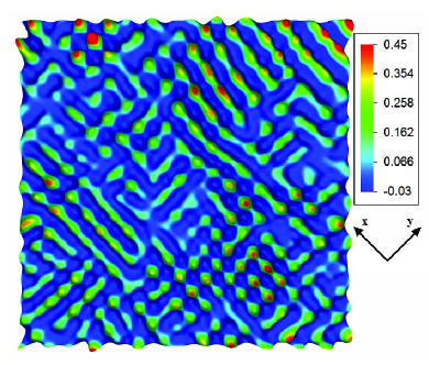
Figure 7: (color online) LDOS integrated in energy up to $E=+15meV$. [Color scale is arbitrary.] Both $\xi_{orient}$ and $\xi_{CDW}$ are quite small, suggestive that the system is in a disorder-pinned, fluctuating phase.

VII Conclusions

There are many circumstances in which charge order plays a significant role in the physics of electronically interesting materials. Depending on the situation, different aspects of the physics may be responsible for the choice of the characteristic period of the charge order; for instance, it can be determined by Fermi surface nesting (as in a Peierls transition), by a small deviation from a commensurate electron density (which fixes a concentration of discommensurations), or by some form of Coulomb frustrated phase separation. Working backwards, measurements of the period of the charge order as a function of parameters (temperature, pressure, doping, …) can shed light on the mechanism of charge ordering.

The physics that determines the ultimate pattern of charge order is still more subtle. For instance, for adsorbates on graphite, the sign of the energy of intersection determines whether the discommensurations form a striped or honeycomb arrangement. Coppersmith et al. (1981) In 2H-TaSe₂, broken hexagonal symmetry has been observed Fleming et al. (1980) in x-ray scattering and TEM Onozuka et al. (1986) (such a system has been studied by McMillian McMillan (1975) using LG methods.) In certain nearly tetragonal rare-earth tellurides, which have been found to form stripe ordered phases, Laverock et al. (2005); DiMasi et al. (1995) this can be shown to be a consequence of some fairly general features of the geometry of the nested portions of the Fermi surface so long as the transition temperature is sufficiently high.Yao et al. (2006)

In the cuprates, calculations of the structures originating from Coulomb-frustrated phase separation,Löw et al. (1994) DMRG calculations on t-J ladders,White and Scalapino (2004) and Hartree-Fock calculations on the Hubbard modelZaanen and Gunnarsson (1989); Schulz (1990); Machida (1989) all suggest that stripe order is typically preferred over checkerboard order. Conversely, the Coulomb repulsion between dilute doped holes, or between dilute Cooper pairs favor a more isotropic (Wigner crystalline) arrangement of charges with more of a checkerboard structure.Chen et al. (2004); Komiya et al. (2005); Fu et al. (2004); Fine (2004) Thus, resolving the nature of the preferred structure of the charge ordered states in the cuprates, at the least, teaches us something about the mechanism of charge ordering in these materials.

On the basis of our present analysis, we feel that there is compelling evidence that most, and possibly all, of the charge order and incipient charge order seen in hole-doped cuprates is preferentially striped. We also conclude that most of the structure seen in STM studies is disorder pinned versions of what would, in the clean limit, be fluctuating stripes, rather than true, static stripe order.

Note: After this work was completed we received a draft of a paper by del Maestro and coworkersMaestro et al. (2006) who discuss similar ideas to the ones we present in this paper. We thank these authors for sharing their work with us prior to publication. After this paper was submitted for publication M. Vojta pointed out to us that in a very recent paper he and his coworkers considered the effects of slow thermal fluctuations of stripe and checkerboard charge order on the magnetic susceptibility of disorder-free high $T_{c}$ cuprates.Vojta et al. (2005).

Note added: While this paper was being refereed a new neutron scattering study of LNSCO became availableChristensen et al. (2006), which confirmed the existence of unidirectional charge order (stripe) and collinear spin order in this material, in agreement with the results and interpretation of Ref.[Tranquada et al., 1995].