[

Electronic structure of kinetic energy driven superconductors

Abstract

Within the framework of the kinetic energy driven superconductivity, we study the electronic structure of cuprate superconductors. It is shown that the spectral weight of the electron spectrum in the antinodal point of the Brillouin zone decreases as the temperature is increased. With increasing the doping concentration, this spectral weigh increases, while the position of the sharp superconducting quasiparticle peak moves to the Fermi energy. In analogy to the normal-state case, the superconducting quasiparticles around the antinodal point disperse very weakly with momentum. Our results also show that the striking behavior of the superconducting coherence of the quasiparticle peaks is intriguingly related to the strong coupling between the superconducting quasiparticles and collective magnetic excitations.

]

The parent compounds of cuprate superconductors are the Mott insulators with an antiferromagnetic (AF) long-range order (AFLRO), then changing the carrier concentration by ionic substitution or increasing the oxygen content turns these compounds into the superconducting (SC)-state leaving the AF short-range correlation still intact [1, 2]. The single common feature of cuprate superconductors is the presence of the two-dimensional CuO₂ plane [1, 2], and it seems evident that the unusual behaviors of cuprate superconductors are dominated by this CuO₂ plane [3]. This layered crystal structure leads to that cuprates superconductors are highly anisotropic materials, then the electron spectral function $A({\bf k},\omega)$ is dependent on the in-plane momentum [4, 5, 6]. Experimentally, an agreement has emerged that at least in the SC-state, the electronic quasiparticle excitations are well defined and are the entities participating in the SC pairing [4, 5, 6, 7, 8, 9]. According to a comparison of the density of states as measured by scanning tunnelling microscopy [10] and angle-resolved photoemission spectroscopy (ARPES) spectral function [4, 11] at the antinodal point, i.e., the $[\pi,0]$ point of the Brillouin zone, on identical samples, it has been shown that there is the presence of a shallow extended saddle point in the $[\pi,0]$ point [4, 5, 6], where the d-wave SC gap function is maximal, then the most contributions of the electron spectral function come from the $[\pi,0]$ point [4, 5, 6, 11]. Moreover, recent improvements in the resolution of ARPES experiments allowed for an experimental verification of the particle-hole coherence in the SC-state and Bogoliubov-quasiparticle nature of the sharp SC quasiparticle peak near the $[\pi,0]$ point [12, 7]. It is striking that in spite of the high temperature SC mechanism and observed exotic magnetic scattering [13, 14, 15] in cuprate superconductors, these ARPES experimental results [12, 7] show that the SC coherence of the quasiparticle peak is described by the simple Bardeen-Cooper-Schrieffer (BCS) formalism [16]. It is thus established that the electron spectral function around the $[\pi,0]$ point dramatically changes with the doping concentration, and has a close relation to superconductivity.

Recently, we have developed a kinetic energy driven SC mechanism [17] based on the charge-spin separation (CSS) fermion-spin theory [18], where the dressed holon-spin interaction from the kinetic energy term induces the dressed holon pairing state by exchanging spin excitations, then the electron Cooper pairs originating from the dressed holon pairing state are due to the charge-spin recombination, and their condensation reveals the SC ground-state. In particular, this SC-state is controlled by both SC gap function and quasiparticle coherence, then the maximal SC transition temperature occurs around the optimal doping, and decreases in both underdoped and overdoped regimes [19]. Within this framework of the kinetic energy driven superconductivity, we [19] have calculated the dynamical spin structure factor, and qualitatively reproduced all main features of inelastic neutron scattering experiments on cuprate superconductors, including the energy dependence of the incommensurate magnetic scattering at both low and high energies and commensurate resonance at intermediate energy [13, 14, 15]. It is believed that both experiments from ARPES and inelastic neutron scattering measurements produce interesting data that introduce important constraints on the microscopic models and SC theories for cuprate superconductors [4, 5, 6, 13, 14, 15]. In this Letter, we study the electronic structure of cuprate superconductors under the kinetic energy driven SC mechanism. Within the $t$-$t^{\prime}$-$J$ model, we have performed a systematic calculation for the electron spectral function in the SC-state, and results show that the spectral weight in the $[\pi,0]$ point increases with increasing doping, and decreases with increasing temperatures. Moreover, the position of the sharp SC quasiparticle peak in the $[\pi,0]$ point moves to the Fermi energy as doping is increased. In analogy to the normal-state case [20, 21], the SC quasiparticles around the $[\pi,0]$ point disperse very weakly with momentum. Our results also show that the striking behavior of the SC coherence of the quasiparticle peaks is intriguingly related to the strong coupling between the SC quasiparticles and collective magnetic excitations.

In cuprate superconductors, the characteristic feature is the presence of the CuO₂ plane [1, 2] as mentioned above. It has been shown from ARPES experiments that the essential physics of the doped CuO₂ plane is properly accounted by the $t$-$t^{\prime}$-$J$ model on a square lattice [4, 22],

$$H = -t\sum_{i\hat{\eta}\sigma}C^{\dagger}_{i\sigma}C_{i+\hat{\eta}\sigma}+t^{\prime}\sum_{i\hat{\tau}\sigma}C^{\dagger}_{i\sigma}C_{i+\hat{\tau}\sigma}$$ (1)

$$+ \mu\sum_{i\sigma}C^{\dagger}_{i\sigma}C_{i\sigma}+J\sum_{i\hat{\eta}}{\bf S}_{i}\cdot{\bf S}_{i+\hat{\eta}},$$ (2)

where $\hat{\eta}=\pm\hat{x},\pm\hat{y}$, $\hat{\tau}=\pm\hat{x}\pm\hat{y}$, $C^{\dagger}_{i\sigma}$ ($C_{i\sigma}$) is the electron creation (annihilation) operator, ${\bf S}_{i}=C^{\dagger}_{i}{\vec{\sigma}}C_{i}/2$ is spin operator with ${\vec{\sigma}}=(\sigma_{x},\sigma_{y},\sigma_{z})$ as Pauli matrices, and $\mu$ is the chemical potential. This $t$-$t^{\prime}$-$J$ model is subject to an important local constraint $\sum_{\sigma}C^{\dagger}_{i\sigma}C_{i\sigma}\leq 1$ to avoid the double occupancy. The strong electron correlation in the $t$-$t^{\prime}$-$J$ model manifests itself by this local constraint [3], which can be treated properly in analytical calculations within the CSS fermion-spin theory [18], where the constrained electron operators are decoupled as $C_{i\uparrow}=h^{\dagger}_{i\uparrow}S^{-}_{i}$ and $C_{i\downarrow}=h^{\dagger}_{i\downarrow}S^{+}_{i}$, with the spinful fermion operator $h_{i\sigma}=e^{-i\Phi_{i\sigma}}h_{i}$ describes the charge degree of freedom together with some effects of spin configuration rearrangements due to the presence of the doped hole itself (dressed holon), while the spin operator $S_{i}$ describes the spin degree of freedom (spin), then the electron local constraint for the single occupancy, $\sum_{\sigma}C^{\dagger}_{i\sigma}C_{i\sigma}=S^{+}_{i}h_{i\uparrow}h^{\dagger}_{i\uparrow}S^{-}_{i}+S^{-}_{i}h_{i\downarrow}h^{\dagger}_{i\downarrow}S^{+}_{i}=h_{i}h^{\dagger}_{i}(S^{+}_{i}S^{-}_{i}+S^{-}_{i}S^{+}_{i})=1-h^{\dagger}_{i}h_{i}\leq 1$, is satisfied in analytical calculations. Moreover, these dressed holon and spin are gauge invariant [18], and in this sense, they are real and can be interpreted as the physical excitations [23]. Although in common sense $h_{i\sigma}$ is not a real spinful fermion, it behaves like a spinful fermion. In this CSS fermion-spin representation, the low-energy behavior of the $t$-$t^{\prime}$-$J$ model (1) can be expressed as,

$$H = -t\sum_{i\hat{\eta}}(h_{i\uparrow}S^{+}_{i}h^{\dagger}_{i+\hat{\eta}\uparrow}S^{-}_{i+\hat{\eta}}+h_{i\downarrow}S^{-}_{i}h^{\dagger}_{i+\hat{\eta}\downarrow}S^{+}_{i+\hat{\eta}})$$ (3)

$$+ t^{\prime}\sum_{i\hat{\tau}}(h_{i\uparrow}S^{+}_{i}h^{\dagger}_{i+\hat{\tau}\uparrow}S^{-}_{i+\hat{\tau}}+h_{i\downarrow}S^{-}_{i}h^{\dagger}_{i+\hat{\tau}\downarrow}S^{+}_{i+\hat{\tau}})$$ (4)

$$- \mu\sum_{i\sigma}h^{\dagger}_{i\sigma}h_{i\sigma}+J_{{\rm eff}}\sum_{i\hat{\eta}}{\bf S}_{i}\cdot{\bf S}_{i+\hat{\eta}},$$ (5)

with $J_{{\rm eff}}=(1-\delta)^{2}J$, and $\delta=\langle h^{\dagger}_{i\sigma}h_{i\sigma}\rangle=\langle h^{\dagger}_{i}h_{i}\rangle$ is the doping concentration. As an important consequence, the kinetic energy terms in the $t$-$t^{\prime}$-$J$ model have been transferred as the dressed holon-spin interactions, this reflects that even the kinetic energy terms in the $t$-$t^{\prime}$-$J$ Hamiltonian have strong Coulombic contributions due to the restriction of no doubly occupancy of a given site. In cuprate superconductors, the SC-state still is characterized by electron Cooper pairs as in the conventional superconductors, forming SC quasiparticles [24]. On the other hand, the range of the SC gap function and pairing force in the real space have been studied experimentally [25, 26]. The early ARPES measurements [25] showed that in the real space the gap function and pairing force have a range of one lattice spacing. However, the recent ARPES measurements [26] indicated that in the underdoped regime the presence of the higher harmonic term ${\rm cos}(2k_{x})-{\rm cos}(2k_{y})$ in the SC gap function. Since the higher harmonic term ${\rm cos}(2k_{x})-{\rm cos}(2k_{y})$ is closely related to the next nearest neighbor interaction, just as the simple ${\rm cos}k_{x}-{\rm cos}k_{y}$ form in the SC gap function is closely related to the nearest neighbor interaction, then the higher harmonics imply an increase in the range of the pairing interaction [26]. In other words, the pairing interaction becomes more long range in the underdoped regime. These higher harmonics are doping dependent, and vanish in the overdoped regime. In particular, the SC gap anisotropy due to the deviations from the simple ${\rm cos}k_{x}-{\rm cos}k_{y}$ form renormalizes the slope of the superfluid density [26]. Although the quantitative description of the SC properties of cuprate superconductors in the underdoped regime needs to consider these higher harmonic effects, the qualitative SC properties are dominated by the gap function with the simple ${\rm cos}k_{x}-{\rm cos}k_{y}$ form [26]. As a qualitative discussions of the electronic structure of cuprate superconductors in this Letter, we do not take into account the higher harmonics in the SC gap function, and only focus on the SC gap function with the simple ${\rm cos}k_{x}-{\rm cos}k_{y}$ form. In this case, we can express the SC order parameter for the electron Cooper pair in the CSS fermion-spin representation as,

$$\Delta = \langle C^{\dagger}_{i\uparrow}C^{\dagger}_{i+\hat{\eta}\downarrow}-C^{\dagger}_{i\downarrow}C^{\dagger}_{i+\hat{\eta}\uparrow}\rangle$$ (6)

$$= \langle h_{i\uparrow}h_{i+\hat{\eta}\downarrow}S^{+}_{i}S^{-}_{i+\hat{\eta}}-h_{i\downarrow}h_{i+\hat{\eta}\uparrow}S^{-}_{i}S^{+}_{i+\hat{\eta}}\rangle$$ (7)

$$= -\chi_{1}\Delta_{h},$$ (8)

where the spin correlation function $\chi_{1}=\langle S_{i}^{+}S_{i+\hat{\eta}}^{-}\rangle$, and dressed holon pairing order parameter $\Delta_{h}=\langle h_{i+\hat{\eta}\downarrow}h_{i\uparrow}-h_{i+\hat{\eta}\uparrow}h_{i\downarrow}\rangle$. The above result in Eq. (3) shows that the SC order parameter is determined by the dressed holon pairing amplitude, and is proportional to the number of doped holes, and not to the number of electrons. In this case, although the SC order parameter measures the strength of the binding of electrons into electron Cooper pairs, it depends on the doping concentration, and is similar to the doping dependent behavior of the upper critical field [27]. In superconductors, the upper critical field is defined as the critical field that destroys the SC-state at the zero temperature for a given doping concentration. This indicates that the upper critical field also measures the strength of the binding of electrons into Cooper pairs like the SC gap parameter [27]. In other words, both SC gap parameter and upper critical field should have a similar doping dependence [27]. Within the Eliashberg’s strong coupling theory [28], we [17] have shown that the dressed holon-spin interaction can induce the dressed holon pairing state (then the electron Cooper pairing state) by exchanging spin excitations in the higher power of the doping concentration. Following our previous discussions [17], the self-consistent equations that satisfied by the full dressed holon diagonal and off-diagonal Green’s functions are expressed as [28],

$$g({\bf k},\omega) = g^{(0)}({\bf k},\omega)+g^{(0)}({\bf k},\omega)[\Sigma^{(h)}_{1}({\bf k},\omega)g({\bf k},\omega)$$ (10)

$$- \Sigma^{(h)}_{2}(-{\bf k},-\omega)\Im^{\dagger}({\bf k},\omega)],$$ (11)

$$\Im^{\dagger}({\bf k},\omega) = g^{(0)}(-{\bf k},-\omega)[\Sigma^{(h)}_{1}(-{\bf k},-\omega)\Im^{\dagger}(-{\bf k},-\omega)$$ (12)

$$+ \Sigma^{(h)}_{2}(-{\bf k},-\omega)g({\bf k},\omega)],$$ (13)

respectively, where the mean-field (MF) dressed holon diagonal Green’s function [18] $g^{(0)-1}({\bf k},\omega)=\omega-\xi_{{\bf k}}$, with the MF dressed holon excitation spectrum $\xi_{{\bf k}}=Zt\chi_{1}\gamma_{{\bf k}}-Zt^{\prime}\chi_{2}\gamma_{{\bf k}}^{\prime}-\mu$, where $\gamma_{{\bf k}}=(1/Z)\sum_{\hat{\eta}}e^{i{\bf k}\cdot\hat{\eta}}$, $\gamma_{{\bf k}}^{\prime}=(1/Z)\sum_{\hat{\tau}}e^{i{\bf k}\cdot\hat{\tau}}$, $Z$ is the number of the nearest neighbor or next nearest neighbor sites, the spin correlation function $\chi_{2}=\langle S_{i}^{+}S_{i+\hat{\tau}}^{-}\rangle$, while the dressed holon self-energies are obtained from the spin bubble as [17, 19],

$$\Sigma^{(h)}_{1}( {\bf k} ,i\omega_{n})={1\over N^{2}}\sum_{{\bf p,p^{\prime}}}\Lambda^{2}_{{\bf p+p^{\prime}+k}}{1\over\beta}\sum_{ip_{m}}g({\bf p+k},ip_{m}+i\omega_{n})$$ (15)

$$\times {1\over\beta}\sum_{ip^{\prime}_{m}}D^{(0)}({\bf p^{\prime}},ip^{\prime}_{m})D^{(0)}({\bf p^{\prime}+p},ip^{\prime}_{m}+ip_{m}),$$ (16)

$$\Sigma^{(h)}_{2}( {\bf k} ,i\omega_{n})={1\over N^{2}}\sum_{{\bf p,p^{\prime}}}\Lambda^{2}_{{\bf p+p^{\prime}+k}}{1\over\beta}\sum_{ip_{m}}\Im({\bf p+k},ip_{m}+i\omega_{n})$$ (17)

$$\times {1\over\beta}\sum_{ip^{\prime}_{m}}D^{(0)}({\bf p^{\prime}},ip^{\prime}_{m})D^{(0)}({\bf p^{\prime}+p},ip^{\prime}_{m}+ip_{m}),$$ (18)

with $\Lambda_{{\bf k}}=Zt\gamma_{{\bf k}}-Zt^{\prime}\gamma_{{\bf k}}^{\prime}$, $N$ is the number of sites, and the MF spin Green’s function [17, 19],

$$D^{(0)}({\bf p},\omega)={B_{{\bf p}}\over 2\omega_{{\bf p}}}\left({1\over\omega-\omega_{{\bf p}}}-{1\over\omega+\omega_{{\bf p}}}\right),$$ (19)

where $B_{{\bf p}}=2\lambda_{1}(A_{1}\gamma_{{\bf p}}-A_{2})-\lambda_{2}(2\chi^{z}_{2}\gamma_{{\bf p}}^{\prime}-\chi_{2})$, $\lambda_{1}=2ZJ_{eff}$, $\lambda_{2}=4Z\phi_{2}t^{\prime}$, $A_{1}=\epsilon\chi^{z}_{1}+\chi_{1}/2$, $A_{2}=\chi^{z}_{1}+\epsilon\chi_{1}/2$, $\epsilon=1+2t\phi_{1}/J_{{\rm eff}}$, the dressed holon’s particle-hole parameters $\phi_{1}=\langle h^{\dagger}_{i\sigma}h_{i+\hat{\eta}\sigma}\rangle$ and $\phi_{2}=\langle h^{\dagger}_{i\sigma}h_{i+\hat{\tau}\sigma}\rangle$, the spin correlation functions $\chi^{z}_{1}=\langle S_{i}^{z}S_{i+\hat{\eta}}^{z}\rangle$ and $\chi^{z}_{2}=\langle S_{i}^{z}S_{i+\hat{\tau}}^{z}\rangle$, and the MF spin excitation spectrum,

$$\omega^{2}_{{\bf p}} = \lambda_{1}^{2}[(A_{4}-\alpha\epsilon\chi^{z}_{1}\gamma_{{\bf p}}-{1\over 2Z}\alpha\epsilon\chi_{1})(1-\epsilon\gamma_{{\bf p}})$$ (20)

$$+ {1\over 2}\epsilon(A_{3}-{1\over 2}\alpha\chi^{z}_{1}-\alpha\chi_{1}\gamma_{{\bf p}})(\epsilon-\gamma_{{\bf p}})]$$ (21)

$$+ \lambda_{2}^{2}[\alpha(\chi^{z}_{2}\gamma_{{\bf p}}^{\prime}-{3\over 2Z}\chi_{2})\gamma_{{\bf p}}^{\prime}+{1\over 2}(A_{5}-{1\over 2}\alpha\chi^{z}_{2})]$$ (22)

$$+ \lambda_{1}\lambda_{2}[\alpha\chi^{z}_{1}(1-\epsilon\gamma_{{\bf p}})\gamma_{{\bf p}}^{\prime}+{1\over 2}\alpha(\chi_{1}\gamma_{{\bf p}}^{\prime}-C_{3})(\epsilon-\gamma_{{\bf p}})$$ (23)

$$+ \alpha\gamma_{{\bf p}}^{\prime}(C^{z}_{3}-\epsilon\chi^{z}_{2}\gamma_{{\bf p}})-{1\over 2}\alpha\epsilon(C_{3}-\chi_{2}\gamma_{{\bf p}})],$$ (24)

with $A_{3}=\alpha C_{1}+(1-\alpha)/(2Z)$, $A_{4}=\alpha C^{z}_{1}+(1-\alpha)/(4Z)$, $A_{5}=\alpha C_{2}+(1-\alpha)/(2Z)$, and the spin correlation functions $C_{1}=(1/Z^{2})\sum_{\hat{\eta},\hat{\eta^{\prime}}}\langle S_{i+\hat{\eta}}^{+}S_{i+\hat{\eta^{\prime}}}^{-}\rangle$, $C^{z}_{1}=(1/Z^{2})\sum_{\hat{\eta},\hat{\eta^{\prime}}}\langle S_{i+\hat{\eta}}^{z}S_{i+\hat{\eta^{\prime}}}^{z}\rangle$, $C_{2}=(1/Z^{2})\sum_{\hat{\tau},\hat{\tau^{\prime}}}\langle S_{i+\hat{\tau}}^{+}S_{i+\hat{\tau^{\prime}}}^{-}\rangle$, $C_{3}=(1/Z)\sum_{\hat{\tau}}\langle S_{i+\hat{\eta}}^{+}S_{i+\hat{\tau}}^{-}\rangle$, and $C^{z}_{3}=(1/Z)\sum_{\hat{\tau}}\langle S_{i+\hat{\eta}}^{z}S_{i+\hat{\tau}}^{z}\rangle$. In order to satisfy the sum rule of the correlation function $\langle S^{+}_{i}S^{-}_{i}\rangle=1/2$ in the case without AFLRO, an important decoupling parameter $\alpha$ has been introduced in the MF calculation [17, 18], which can be regarded as the vertex correction.

In the previous discussions [17, 19], we have shown that both doping and temperature dependence of the pairing force and dressed holon gap function are incorporated into the self-energy function $\Sigma^{(h)}_{2}({\bf k},\omega)$. In this case, the self-energy function $\Sigma^{(h)}_{2}({\bf k},\omega)$ describes the effective dressed holon pair gap function. On the other hand, the self-energy function $\Sigma^{(h)}_{1}({\bf k},\omega)$ renormalizes the MF dressed holon spectrum, and thus it describes the quasiparticle coherence. Furthermore, $\Sigma^{(h)}_{2}({\bf k},\omega)$ is an even function of $\omega$, while $\Sigma^{(h)}_{1}({\bf k},\omega)$ is not. For the convenience, we break $\Sigma^{(h)}_{1}({\bf k},\omega)$ up into its symmetric and antisymmetric parts as, $\Sigma^{(h)}_{1}({\bf k},\omega)=\Sigma^{(h)}_{1e}({\bf k},\omega)+\omega\Sigma^{(h)}_{1o}({\bf k},\omega)$, then both $\Sigma^{(h)}_{1e}({\bf k},\omega)$ and $\Sigma^{(h)}_{1o}({\bf k},\omega)$ are even functions of $\omega$. According to the Eliashberg’s strong coupling theory [28], we define the quasiparticle coherent weight as $Z^{-1}_{F}({\bf k},\omega)=1-\Sigma^{(h)}_{1o}({\bf k},\omega)$. Since we only discuss the low-energy behavior of cuprate superconductors, then the effective dressed holon pair gap function and quasiparticle coherent weight can be discussed in the static limit, i.e., $\bar{\Delta}_{h}({\bf k})=\Sigma^{(h)}_{2}({\bf k},\omega)\mid_{\omega=0}$, $Z^{-1}_{F}({\bf k})=1-\Sigma^{(h)}_{1o}({\bf k},\omega)\mid_{\omega=0}$, and $\Sigma^{(h)}_{1e}({\bf k})=\Sigma^{(h)}_{1e}({\bf k},\omega)\mid_{\omega=0}$. Although $Z_{F}({\bf k})$ and $\Sigma^{(h)}_{1e}({\bf k})$ still are a function of ${\bf k}$, the wave vector dependence may be unimportant [28]. From ARPES experiments [4, 5, 6], it has been shown that in the SC-state, the lowest energy states are located at the $[\pi,0]$ point, which indicates that the majority contribution for the electron spectrum comes from the $[\pi,0]$ point. In this case, the wave vector ${\bf k}$ in $Z_{F}({\bf k})$ and $\Sigma^{(h)}_{1e}({\bf k})$ can be chosen as $Z^{-1}_{F}=1-\Sigma^{(h)}_{1o}({\bf k})\mid_{{\bf k}=[\pi,0]}$ and $\Sigma^{(h)}_{1e}=\Sigma^{(h)}_{1e}({\bf k})\mid_{{\bf k}=[\pi,0]}$. This is different from the previous discussions [19], where the wave vector ${\bf k}$ in $Z_{F}({\bf k})$ and $\Sigma^{(h)}_{1e}({\bf k})$ has been chosen near the nodal point in the Brillouin zone. With the help of the above discussions, the dressed holon diagonal and off-diagonal Green’s functions in Eqs. (4a) and (4b) can be obtained explicitly as,

$$g({\bf k},\omega) = Z_{F}{U^{2}_{h{\bf k}}\over\omega-E_{h{\bf k}}}+Z_{F}{V^{2}_{h{\bf k}}\over\omega+E_{h{\bf k}}},$$ (26)

$$\Im^{\dagger}({\bf k},\omega) = -Z_{F}{\bar{\Delta}_{hZ}({\bf k})\over 2E_{h{\bf k}}}\left({1\over\omega-E_{h{\bf k}}}-{1\over\omega+E_{h{\bf k}}}\right),$$ (27)

where the dressed holon quasiparticle coherence factors $U^{2}_{h{\bf k}}=(1+\bar{\xi_{{\bf k}}}/E_{h{\bf k}})/2$ and $V^{2}_{h{\bf k}}=(1-\bar{\xi_{{\bf k}}}/E_{h{\bf k}})/2$, the renormalized dressed holon excitation spectrum $\bar{\xi_{{\bf k}}}=Z_{F}(\xi_{{\bf k}}+\Sigma^{(h)}_{1e})$, the renormalized dressed holon pair gap function $\bar{\Delta}_{hZ}({\bf k})=Z_{F}\bar{\Delta}_{h}({\bf k})$, and the dressed holon quasiparticle spectrum $E_{h{\bf k}}=\sqrt{\bar{\xi^{2}_{{\bf k}}}+\mid\bar{\Delta}_{hZ}({\bf k})\mid^{2}}$. This dressed holon quasiparticle is the excitation of a single dressed holon ”adorned” with the attractive interaction between paired dressed holons, while the $Z_{F}$ reduces the dressed holon (then electron) quasiparticle bandwidth, and then the energy scale of the electron quasiparticle band is controlled by the magnetic interaction $J$. On the other hand, cuprate superconductors are characterized by an overall d-wave pairing symmetry [24]. In particular, we [19] have shown within the $t$-$J$ type model that the electron Cooper pairs have a dominated d-wave symmetry over a wide range of the doping concentration, around the optimal doping. Therefore in the following discussions, we consider the d-wave case, i.e., $\bar{\Delta}_{hZ}({\bf k})=\bar{\Delta}_{hZ}\gamma^{(d)}_{{\bf k}}$, with $\gamma^{(d)}_{{\bf k}}=({\rm cos}k_{x}-{\rm cos}k_{y})/2$. In this case, the dressed holon effective gap parameter and quasiparticle coherent weight in Eqs. (5a) and (5b) satisfy the following two equations,

$$1 = {1\over N^{3}}\sum_{{\bf k,p,p^{\prime}}}\Lambda^{2}_{{\bf p+k}}\gamma^{(d)}_{{\bf k-p^{\prime}+p}}\gamma^{(d)}_{{\bf k}}{Z^{2}_{F}\over E_{h{\bf k}}}{B_{{\bf p}}B_{{\bf p^{\prime}}}\over\omega_{{\bf p}}\omega_{{\bf p^{\prime}}}}$$ (29)

$$\times \left({F^{(1)}_{1}({\bf k,p,p^{\prime}})\over(\omega_{{\bf p^{\prime}}}-\omega_{{\bf p}})^{2}-E^{2}_{h{\bf k}}}-{F^{(2)}_{1}({\bf k,p,p^{\prime}})\over(\omega_{{\bf p^{\prime}}}+\omega_{{\bf p}})^{2}-E^{2}_{h{\bf k}}}\right),$$ (30)

$${1\over Z}_{F} = 1+{1\over N^{2}}\sum_{{\bf p,p^{\prime}}}\Lambda^{2}_{{\bf p}+{\bf k}_{0}}Z_{F}{B_{{\bf p}}B_{{\bf p^{\prime}}}\over 4\omega_{{\bf p}}\omega_{{\bf p^{\prime}}}}$$ (31)

$$\times \left({F^{(1)}_{2}({\bf p,p^{\prime}})\over(\omega_{{\bf p}}-\omega_{{\bf p^{\prime}}}-E_{h{\bf p-p^{\prime}+k_{0}}})^{2}}\right.$$ (32)

$$+ {F^{(2)}_{2}({\bf p,p^{\prime}})\over(\omega_{{\bf p}}-\omega_{{\bf p^{\prime}}}+E_{h{\bf p-p^{\prime}+k_{0}}})^{2}}$$ (33)

$$+ {F^{(3)}_{2}({\bf p,p^{\prime}})\over(\omega_{{\bf p}}+\omega_{{\bf p^{\prime}}}-E_{h{\bf p-p^{\prime}+k_{0}}})^{2}}$$ (34)

$$+ \left.{F^{(4)}_{2}({\bf p,p^{\prime}})\over(\omega_{{\bf p}}+\omega_{{\bf p^{\prime}}}+E_{h{\bf p-p^{\prime}+k_{0}}})^{2}}\right),$$ (35)

respectively, where ${\bf k}_{0}=[\pi,0]$, $F^{(1)}_{1}({\bf k,p,p^{\prime}})=(\omega_{{\bf p^{\prime}}}-\omega_{{\bf p}})[n_{B}(\omega_{{\bf p}})-n_{B}(\omega_{{\bf p^{\prime}}})][1-2n_{F}(E_{h{\bf k}})]+E_{h{\bf k}}[n_{B}(\omega_{{\bf p^{\prime}}})n_{B}(-\omega_{{\bf p}})+n_{B}(\omega_{{\bf p}})n_{B}(-\omega_{{\bf p^{\prime}}})]$, $F^{(2)}_{1}({\bf k,p,p^{\prime}})=(\omega_{{\bf p^{\prime}}}+\omega_{{\bf p}})[n_{B}(-\omega_{{\bf p^{\prime}}})-n_{B}(\omega_{{\bf p}})][1-2n_{F}(E_{h{\bf k}})]+E_{h{\bf k}}[n_{B}(\omega_{{\bf p^{\prime}}})n_{B}(\omega_{{\bf p}})+n_{B}(-\omega_{{\bf p^{\prime}}})n_{B}(-\omega_{{\bf p}})]$, $F^{(1)}_{2}({\bf p,p^{\prime}})=n_{F}(E_{h{\bf p-p^{\prime}+k_{0}}})[n_{B}(\omega_{{\bf p^{\prime}}})-n_{B}(\omega_{{\bf p}})]-n_{B}(\omega_{{\bf p}})n_{B}(-\omega_{{\bf p^{\prime}}})$, $F^{(2)}_{2}({\bf p,p^{\prime}})=n_{F}(E_{h{\bf p-p^{\prime}+k_{0}}})[n_{B}(\omega_{{\bf p}})-n_{B}(\omega_{{\bf p^{\prime}}})]-n_{B}(\omega_{{\bf p^{\prime}}})n_{B}(-\omega_{{\bf p}})$, $F^{(3)}_{2}({\bf p,p^{\prime}})=n_{F}(E_{h{\bf p-p^{\prime}+k_{0}}})[n_{B}(\omega_{{\bf p^{\prime}}})-n_{B}(-\omega_{{\bf p}})]+n_{B}(\omega_{{\bf p}})n_{B}(\omega_{{\bf p^{\prime}}})$, and $F^{(4)}_{2}({\bf p,p^{\prime}})=n_{F}(E_{h{\bf p-p^{\prime}+k_{0}}})[n_{B}(-\omega_{{\bf p^{\prime}}})-n_{B}(\omega_{{\bf p}})]+n_{B}(-\omega_{{\bf p}})n_{B}(-\omega_{{\bf p^{\prime}}})$. These two equations must be solved simultaneously with other self-consistent equations [17, 18, 19], then all order parameters, decoupling parameter $\alpha$, and chemical potential $\mu$ are determined by the self-consistent calculation. In this sense, our above calculations are controllable without using adjustable parameters.

According to the dressed holon off-diagonal Green’s function (8b), the dressed holon pair gap function is obtained as $\Delta_{h}({\bf k})=-(1/\beta)\sum_{i\omega_{n}}\Im^{\dagger}({\bf k},i\omega_{n})$. In the previous discussions [17], it has been shown that this dressed holon pairing state originating from the kinetic energy terms by exchanging spin excitations also leads to form the electron Cooper pairing state. For discussions of the electronic structure in the SC-state, we need to calculate the electron diagonal and off-diagonal Green’s functions $G(i-j,t-t^{\prime})=\langle\langle C_{i\sigma}(t);C^{\dagger}_{j\sigma}(t^{\prime})\rangle\rangle$ and $\Gamma^{\dagger}(i-j,t-t^{\prime})=\langle\langle C^{\dagger}_{i\uparrow}(t);C^{\dagger}_{j\downarrow}(t^{\prime})\rangle\rangle$, which are the convolutions of the spin Green’s function and dressed holon diagonal and off-diagonal Green’s functions in the CSS fermion-spin theory, and can be obtained in terms of the MF spin Green’s function (6) and dressed holon diagonal and off-diagonal Green’s functions (8a) and (8b) as,

$$G({\bf k},\omega) = {1\over N}\sum_{{\bf p}}Z_{F}{B_{{\bf p}}\over 4\omega_{{\bf p}}}\left\{{\rm coth}[{1\over 2}\beta\omega_{{\bf p}}]\right.$$ (37)

$$\times \left({U^{2}_{h{\bf p+k}}\over\omega+E_{h{\bf p+k}}-\omega_{{\bf p}}}+{U^{2}_{h{\bf p+k}}\over\omega+E_{h{\bf p+k}}+\omega_{{\bf p}}}\right.$$ (38)

$$+ \left.{V^{2}_{h{\bf p+k}}\over\omega-E_{h{\bf p+k}}+\omega_{{\bf p}}}+{V^{2}_{h{\bf p+k}}\over\omega-E_{h{\bf p+k}}-\omega_{{\bf p}}}\right)$$ (39)

$$+ {\rm tanh}[{1\over 2}\beta E_{h{\bf p+k}}]\left({U^{2}_{h{\bf p+k}}\over\omega+E_{h{\bf p+k}}+\omega_{{\bf p}}}\right.$$ (40)

$$- {U^{2}_{h{\bf p+k}}\over\omega+E_{h{\bf p+k}}-\omega_{{\bf p}}}+{V^{2}_{h{\bf p+k}}\over\omega-E_{h{\bf p+k}}-\omega_{{\bf p}}}$$ (41)

$$- \left.\left.{V^{2}_{h{\bf p+k}}\over\omega-E_{h{\bf p+k}}+\omega_{{\bf p}}}\right)\right\},$$ (42)

$$\Gamma^{\dagger}({\bf k},\omega) = {1\over N}\sum_{{\bf p}}Z_{F}{\bar{\Delta}_{hZ}({\bf p+k})\over 2E_{h{\bf p+k}}}{B_{{\bf p}}\over 4\omega_{{\bf p}}}\left\{{\rm coth}[{1\over 2}\beta\omega_{{\bf p}}]\right.$$ (43)

$$\times \left({1\over\omega-E_{h{\bf p+k}}-\omega_{{\bf p}}}+{1\over\omega-E_{h{\bf p+k}}+\omega_{{\bf p}}}\right.$$ (44)

$$- \left.{1\over\omega+E_{h{\bf p+k}}+\omega_{{\bf p}}}-{1\over\omega+E_{h{\bf p+k}}-\omega_{{\bf p}}}\right)$$ (45)

$$+ {\rm tanh}[{1\over 2}\beta E_{h{\bf p+k}}]\left({1\over\omega-E_{h{\bf p+k}}-\omega_{{\bf p}}}\right.$$ (46)

$$- {1\over\omega-E_{h{\bf p+k}}+\omega_{{\bf p}}}-{1\over\omega+E_{h{\bf p+k}}+\omega_{{\bf p}}}$$ (47)

$$+ \left.\left.{1\over\omega+E_{h{\bf p+k}}-\omega_{{\bf p}}}\right)\right\},$$ (48)

respectively, these convolutions of the spin Green’s function and dressed holon diagonal and off-diagonal Green’s functions reflect the charge-spin recombination [29], then the electron spectral function $A({\bf k},\omega)=-2{\rm Im}G({\bf k},\omega)$ and SC gap function $\Delta({\bf k})=-(1/\beta)\sum_{i\omega_{n}}\Gamma^{\dagger}({\bf k},i\omega_{n})$ are obtained from the above electron diagonal and off-diagonal Green’s functions as,

$$A({\bf k},\omega) = 2\pi{1\over N}\sum_{{\bf p}}Z_{F}{B_{{\bf p}}\over 4\omega_{{\bf p}}}\left\{{\rm coth}({1\over 2}\beta\omega_{{\bf p}})\right.$$ (50)

$$\times [U^{2}_{h{\bf p+k}}\delta(\omega+E_{h{\bf p+k}}-\omega_{{\bf p}})$$ (51)

$$+ U^{2}_{h{\bf p+k}}\delta(\omega+E_{h{\bf p+k}}+\omega_{{\bf p}})$$ (52)

$$+ V^{2}_{h{\bf p+k}}\delta(\omega-E_{h{\bf p+k}}+\omega_{{\bf p}})$$ (53)

$$+ V^{2}_{h{\bf p+k}}\delta(\omega-E_{h{\bf p+k}}-\omega_{{\bf p}})]$$ (54)

$$+ {\rm tanh}({1\over 2}\beta E_{h{\bf p+k}})[U^{2}_{h{\bf p+k}}\delta(\omega+E_{h{\bf p+k}}+\omega_{{\bf p}})$$ (55)

$$- U^{2}_{h{\bf p+k}}\delta(\omega+E_{h{\bf p+k}}-\omega_{{\bf p}})$$ (56)

$$+ V^{2}_{h{\bf p+k}}\delta(\omega-E_{h{\bf p+k}}-\omega_{{\bf p}})$$ (57)

$$- \left.V^{2}_{h{\bf p+k}}\delta(\omega-E_{h{\bf p+k}}+\omega_{{\bf p}})]\right\},$$ (58)

$$\Delta({\bf k}) = -{1\over N}\sum_{{\bf p}}{Z_{F}\bar{\Delta}_{Zh}({\bf p-k})\over 2E_{h{\bf p-k}}}{\rm tanh}[{1\over 2}\beta E_{h{\bf p-k}}]$$ (59)

$$\times {B_{{\bf p}}\over 2\omega_{{\bf p}}}{\rm coth}[{1\over 2}\beta\omega_{{\bf p}}],$$ (60)

respectively. With the above SC gap function (11b), the SC gap parameter in Eq. (3) is obtained as $\Delta=-\chi_{1}\Delta_{h}$. Since both dressed holon (then electron) pairing gap parameter and pairing interaction in cuprate superconductors are doping dependent, then the experimental observed doping dependence of the SC gap parameter should be an effective SC gap parameter $\bar{\Delta}\sim-\chi_{1}\bar{\Delta}_{h}$. For a complement of the previous analysis of the interplay between the quasiparticle coherence and superconductivity [19], we plot (a) the quasiparticle coherent weight $Z_{F}(T_{c})$, (b) the effective SC gap parameter $\bar{\Delta}$ at temperature $T=0.002J$, and (c) the SC transition temperature $T_{c}$ as a function of the doping concentration for parameters $t/J=2.5$ and $t^{\prime}/J=0.3$ in Fig. 1. For comparison, the corresponding experimental results of the quasiparticle coherent weight in the $[\pi,0]$ point [11], upper critical field [27], and SC transition temperature [30] as a function of the doping concentration are also shown in Fig. 1(a), 1(b), and 1(c), respectively. Although we focus on the quasiparticle coherent weight at the antinodal point in the above discussions, our present results of the doping dependence of the effective SC gap parameter and SC transition temperature are consistent with these of the previous results [19], where it has been focused on the quasiparticle coherent weight near the nodal point. The quasiparticle coherent weight grows linearly with the doping concentration, i.e., $Z_{F}\propto\delta$, which together with the SC gap parameter defined in Eq. (3) show that only $\delta$ number of coherent doped carriers are recovered in the SC-state, consistent with the picture of a doped Mott insulator with $\delta$ holes [3]. In this case, the SC-state of cuprate superconductors is controlled by both SC gap function and quasiparticle coherence [11, 19], then the SC transition temperature increases with increasing doping in the underdoped regime, and reaches a maximum in the optimal doping, then decreases in the overdoped regime. Using an reasonably estimative value of $J\sim 800$K to 1200K in cuprate superconductors [1, 2], the SC transition temperature in the optimal doping is T${}_{c}\approx 0.165J\approx 132{\rm K}\sim 198{\rm K}$, in qualitative agreement with the experimental data [30].

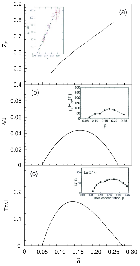
FIG. 1.: (a) The quasiparticle coherent weight $Z_{F}(T_{c})$ in the $[\pi,0]$ point, (b) the effective SC gap parameter $\bar{\Delta}$ at $T=0.002J$, and (c) the SC transition temperature $T_{c}$ as a function of the doping concentration for $t/J=2.5$ and $t^{\prime}/J=0.3$. Inset: the corresponding experimental results of cuprate superconductors taken from Refs. [11], [27], and [30], respectively.

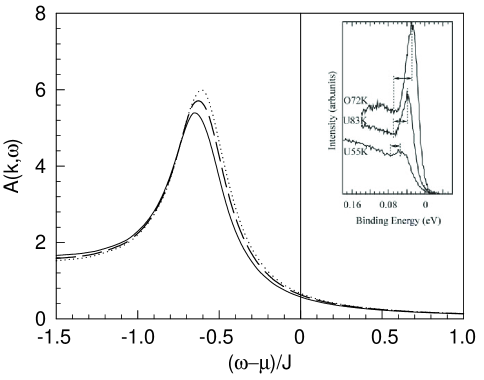
FIG. 2.: The electron spectral function $A({\bf k},\omega)$ in the $[\pi,0]$ point with $\delta=0.09$ (solid line), $\delta=0.12$ (dashed line), and $\delta=0.15$ (dotted line) at $T=0.002J$ for $t/J=2.5$ and $t^{\prime}/J=0.3$. Inset: the experimental result of cuprate superconductors taken from Ref. [9].

Now we are ready to discuss the electronic structure of cuprate superconductors. We have performed a calculation for the electron spectral function (11a), and the results of $A({\bf k},\omega)$ in the $[\pi,0]$ point with the doping concentration $\delta=0.09$ (solid line), $\delta=0.12$ (dashed line), and $\delta=0.15$ (dotted line) at temperature $T=0.002J$ for parameters $t/J=2.5$ and $t^{\prime}/J=0.3$ are plotted in Fig. 2 in comparison with the experimental result [9] (inset). Our results show that there is a sharp SC quasiparticle peak near the electron Fermi energy in the $[\pi,0]$ point, and the position of the SC quasiparticle peak in the doping concentration $\delta=0.15$ is located at $\omega_{{\rm peak}}\approx 0.6J\approx 0.042$eV$\sim 0.06$eV, which is qualitatively consistent with $\omega_{{\rm peak}}\approx 0.03$eV observed [9, 11, 4] in the slightly overdoped cuprate superconductor Bi₂Sr₂CaCu₂O_8+x. Moreover, the electron spectrum is doping dependent. With increasing the doping concentration, the weight of the SC quasiparticle peaks increases, while the position of the SC quasiparticle peak moves to the Fermi energy [9, 4]. Furthermore, we have discussed the temperature dependence of the electron spectrum, and the results of $A({\bf k},\omega)$ in the $[\pi,0]$ point with the doping concentration $\delta=0.15$ at temperature $T=0.002J$ (solid line), $T=0.10J$ (dashed line), and $T=0.15J$ (dotted line) for parameters $t/J=2.5$ and $t^{\prime}/J=0.3$ are plotted in Fig. 3 in comparison with the experimental result [8] (inset). These results show that the spectral weight decreases as temperature is increased, in qualitative agreement with the experimental data [8, 4]. This temperature dependence of the electron spectrum in cuprate superconductors has also been discussed in Ref. [31]. By direct analysis of the ARPES data, they [31] studied the temperature dependence of the electron self-energy, and then indicated that the spectral lineshape in the $[\pi,0]$ point is naturally explained by the coupling of the electrons to a magnetic resonance. Since the intensity of this resonance decreases with temperature, then the coupling of the electrons to this magnetic mode also decreases. As the magnetic resonance intensity decreases, the spin gap in the dynamic susceptibility fills in, which may be responsible for the ”filling in” of the imaginary part of the electron self-energy [31]. The combination of these two effects cause the spectral peak to rapidly broaden with temperature. Our results are also consistent with their results.

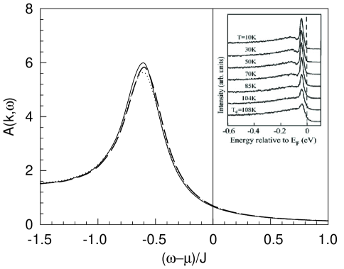
FIG. 3.: The electron spectral function $A({\bf k},\omega)$ in the $[\pi,0]$ point with $\delta=0.15$ at $T=0.002J$ (solid line), $T=0.10J$ (dashed line), and $T=0.15J$ (dotted line) for $t/J=2.5$ and $t^{\prime}/J=0.3$. Inset: the experimental result of cuprate superconductors taken from Ref. [8].

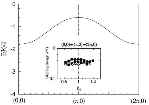
FIG. 4.: The positions of the lowest energy SC quasiparticle peaks in $A({\bf k},\omega)$ as a function of momentum along the direction $[0,0]\rightarrow[\pi,0]\rightarrow[2\pi,0]$ with $\delta=0.15$ at $T=0.002J$ for $t/J=2.5$ and $t^{\prime}/J=0.3$. Inset: the experimental result of cuprate superconductors taken from Ref. [9].

For a better understanding of the anomalous form of the electron spectrum $A({\bf k},\omega)$ as a function of energy $\omega$ for ${\bf k}$ in the vicinity of the $[\pi,0]$ point, we have made a series of calculations for $A({\bf k},\omega)$ around the $[\pi,0]$ point, and the results show that the sharp SC quasiparticle peak persists in a very large momentum space region around the $[\pi,0]$ point. To show this point clearly, we plot the positions of the lowest energy SC quasiparticle peaks in $A({\bf k},\omega)$ as a function of momentum along the direction $[0,0]\rightarrow[\pi,0]\rightarrow[2\pi,0]$ at the doping concentration $\delta=0.15$ with temperature $T=0.002J$ for parameters $t/J=2.5$ and $t^{\prime}/J=0.3$ in Fig. 4 in comparison with the experimental result [9] of the cuprate superconductor Bi₂Sr₂CaCu₂O_8+δ (inset). It is shown that the sharp SC quasiparticle peaks around the $[\pi,0]$ point at low energies disperse very weakly with momentum, which is corresponding to the unusual flat band appeared in the normal-state around the $[\pi,0]$ point [20, 21], and is qualitatively consistent with these obtained from ARPES experimental measurements on doped cuprates [4, 5, 6, 9].

A nature question is why the SC coherence of the SC quasiparticle peak in cuprate superconductors can be described qualitatively in the framework of the kinetic energy driven superconductivity. The reason is that the SC-state in the kinetic energy driven superconductivity is the conventional BCS like [19]. This can be understood from the electron diagonal and off-diagonal Green’s functions in Eqs. (10a) and (10b). Since the spins center around the $[\pi,\pi]$ point in the MF level [17, 18], then the main contributions for the spins comes from the $[\pi,\pi]$ point. In this case, the electron diagonal and off-diagonal Green’s functions in Eqs. (10a) and (10b) can be approximately reduced in terms of $\omega_{{\bf p}=[\pi,\pi]}\sim 0$ and the equation [17, 18] $1/2=\langle S_{i}^{+}S_{i}^{-}\rangle=(1/N)\sum_{{\bf p}}B_{{\bf p}}{\rm coth}(\beta\omega_{{\bf p}}/2)/(2\omega_{{\bf p}})$ as,

$$g({\bf k},\omega) \approx Z_{F}{U^{2}_{{\bf k}}\over\omega-E_{{\bf k}}}+Z_{F}{V^{2}_{{\bf k}}\over\omega+E_{{\bf k}}},$$ (62)

$$\Gamma^{\dagger}({\bf k},\omega) \approx Z_{F}{\bar{\Delta}_{hZ}({\bf k})\over 2E_{{\bf k}}}\left({1\over\omega-E_{{\bf k}}}+{1\over\omega+E_{{\bf k}}}\right),$$ (63)

where the electron quasiparticle coherence factors $U^{2}_{{\bf k}}\approx V^{2}_{h{\bf k+k_{A}}}$ and $V^{2}_{{\bf k}}\approx U^{2}_{h{\bf k+k_{A}}}$, and electron quasiparticle spectrum $E_{{\bf k}}\approx E_{h{\bf k+k_{A}}}$, with ${\bf k_{A}}=[\pi,\pi]$, i.e., the hole-like dressed holon quasiparticle coherence factors $V_{h{\bf k}}$ and $U_{h{\bf k}}$ and hole-like dressed holon quasiparticle spectrum $E_{h{\bf k}}$ have been transferred into the electron quasiparticle coherence factors $U_{{\bf k}}$ and $V_{{\bf k}}$ and electron quasiparticle spectrum $E_{{\bf k}}$, respectively, by the convolutions of the spin Green’s function and dressed holon Green’s functions due to the charge-spin recombination. This means that the dressed holon pairs condense with the d-wave symmetry in a wide range of the doping concentration, then the electron Cooper pairs originating from the dressed holon pairing state are due to the charge-spin recombination, and their condensation automatically gives the electron quasiparticle character. This electron quasiparticle is the excitation of a single electron ”dressed” with the attractive interaction between paired electrons. This is why the basic BCS formalism [16] is still valid in discussions of the doping dependence of the effective SC gap parameter and SC transition temperature, and SC coherence of the quasiparticle peak [12, 7], although the pairing mechanism is driven by the kinetic energy by exchanging spin excitations, and other exotic magnetic scattering [13, 14, 15, 19] is beyond the BCS theory.

In summary, we have studied the electronic structure of cuprate superconductors based on the kinetic energy driven superconductivity. Our results show that the spectral weight of the electron spectrum in the $[\pi,0]$ point decreases as temperature is increased. With increasing the doping concentration, this spectral weight increases, while the position of the sharp SC quasiparticle peak moves to the Fermi energy. In analogy to the normal-state case [20, 21], the SC quasiparticles around the $[\pi,0]$ point disperse very weakly with momentum. Our results also show that the striking behavior of the SC coherence of the quasiparticle peak is intriguingly related to the strong coupling between the SC quasiparticles and collective magnetic excitations.

REFERENCES

[1] See, e.g., Proceedings of Los Alamos
Symposium, edited by K.S. Bedell, D. Coffey, D.E. Meltzer, D.
Pines, and J.R. Schrieffer (Addison-Wesley, Redwood city,
California, 1990).
[2] See, e.g., M.A.Kastner, R.J. Birgeneau, G.
Shiran, and Y. Endoh, Rev. Mod. Phys. 70, 897 (1998), and
referenes therein.
[3] P.W. Anderson, in Frontiers and
Borderlines in Many Particle Physics, edited by R.A. Broglia and
J.R. Schrieffer (North-Holland, Amsterdam, 1987), p. 1; Science
235, 1196 (1987).
[4] See, e.g., A. Damascelli, Z. Hussain, and Z.-X.
Shen, Rev. Mod. Phys. 75, 475 (2003), and referenes therein.
[5] See, e.g., J. Campuzano, M. Norman, M. Randeira,
in Physics of Superconductors, vol. II, edited by K.
Bennemann and J. Ketterson (Springer, Berlin Heidelberg New York,
2004), p. 167, and referenes therein.
[6] See, e.g., J. Fink, S. Borisenko, A. Kordyuk, A.
Koitzsch, J. Geck, V. Zabolotnyy, M. Knupfer, B. Büchner, and H.
Berger, cond-mat/0512307, and referenes therein.
[7] J. Campuzano, H. Ding, M. Norman, M. Randeira,
A. Bellman, T. Mochiku, and K. Kadowaki, Phys. Rev. B 53,
14737 (2003).
[8] D.L. Feng, A. Damascelli, K.M. Shen, N.
Motoyama, D.H. Lu, H. Eisaki, K. Shimizu, J.-i. Shimoyama, K.
Kishio, N. Kaneko, M. Greven, G.D. Gu, X.J. Zhou, C. Kim, F.
Ronning, N.P. Armitage, and Z.-X Shen, Phys. Rev. Lett. 88,
107001 (2002).
[9] J. Campuzano, H. Ding, M. Norman, H. Fretwell,
M. Randeira, A. Kaminski, J. Mesot, T. Takeuchi, T. Sato, T.
Yokoya, T. Takahashi, T. Mochiku, K. Kadowaki, P. Guptasarma, D.
Hinks, Z. Konstantinovic, Z. Li, and H. Raffy, Phys. Rev. Lett.
83, 3709 (1999).
[10] Y. DeWilde, N. Miyakawa, P. Guptasarma, M.
Iavarone, L. Ozyuzer, J. Zasadzinski, P. Romano, D. Hinks, C.
Kendziora, G. Crabrtee, and K. Gray, Phys. Rev. Lett. 80,
153 (1998).
[11] H. Ding, J.R. Engelbrecht, Z. Wang, J.C. Campuzano,
S.C. Wang, H.B. Yang, R. Rogan, T. Takahashi, K. Kadowaki, and
D.G. Hinks, Phys. Rev. Lett. 87, 227001 (2001).
[12] H. Matsui, T. Sato, T. Takahashi, S.C. Wang, H.B.
Yang, H. Ding, T. Fujii, T. Watanabe, and A. Matsuda, Phys. Rev.
Lett. 90, 217002 (2003).
[13] K. Yamada, C.H. Lee, K. Kurahashi, J. Wada, S.
Wakimoto, S. Ueki, H. Kimura, Y. Endoh, S. Hosoya, and G. Shirane,
Phys. Rev. B 57, 6165 (1998).
[14] P. Dai, H.A. Mook, R.D. Hunt, and F. Dog̃an, Phys.
Rev. B63, 54525 (2001); P. Bourges, B. Keimer, S. Pailhés,
L.P. Regnault, Y. Sidis, and C. Ulrich, Physica C 424, 45
(2005).
[15] M. Arai, T. Nishijima, Y. Endoh, T. Egami, S.
Tajima, K. Tomimoto, Y. Shiohara, M. Takahashi, A. Garret, and
S.M. Bennington, Phys. Rev. Lett. 83, 608 (1999); S.M.
Hayden, H.A. Mook, P. Dai, T.G. Perring, and F. Dog̃an, Nature
429, 531 (2004); C. Stock, W.J. Buyers, R.A. Cowley, P.S.
Clegg, R. Coldea, C.D. Frost, R. Liang, D. Peets, D. Bonn, W.N.
Hardy, and R.J. Birgeneau, Phys. Rev. B71, 24522 (2005).
[16] J.R. Schrieffer, Theory of Superconductivity,
Benjamin, New York, 1964.
[17] Shiping Feng, Phys. Rev. B68, 184501
(2003).
[18] Shiping Feng, Jihong Qin, and Tianxing Ma, J.
Phys. Condens. Matter 16, 343 (2004); Shiping Feng, Tianxing
Ma, and Jihong Qin, Mod. Phys. Lett. B17, 361 (2003).
[19] Shiping Feng, Tianxing Ma, and Huaiming Guo,
Physica C 436, 14 (2006); Shiping Feng and Tianxing Ma,
Phys. Lett. A 350, 138 (2006); Shiping Feng and Tianxing Ma,
in New Frontiers in Superconductivity Research, edited by
B.P. Martins (Nova Science Publishers, New York, 2006), Chapter
12, in press, cond-mat/0603148.
[21] D.S. Dessau, Z.X. Shen, D.M. King, D.S. Marshall,
L.W. Lombardo, P.H. Dickinson, A.G. Loeser, J. DiCarlo, C.H. Park,
A. Kapitulnik, and W.E. Spicer, Phys. Rev. Lett. 71, 2781
(1993); Huaiming Guo and Shiping Feng, Phys. Lett. A 355,
473 (2006).
[22] B.O. Wells, Z.X. Shen, A. Matsuura, D.M. King,
M. A. Kastner, M. Greven, and R.J. Birgeneau, Phys. Rev. Lett.
74, 964 (1995); C. Kim, P.J. White, Z.X. Shen, T. Tohyama,
Y. Shibata, S. Maekawa, B.O. Wells, Y.J. Kim, R.J. Birgeneau, and
M.A. Kastner, Phys. Rev. Lett. 80, 4245 (1998).
[23] R.B Laughlin, Phys. Rev. Lett. 79,
1726 (1997); J. Low. Tem. Phys. 99, 443 (1995).
[24] See, e.g., C.C. Tsuei and J.P. Kirtley, Rev. Mod.
Phys. 72, 969 (2000).
[25] Z.X. Shen, D.S. Dessau, B.O. Wells, D.M. King,
W.E. Spicer, A.J. Arko, D. Marshall, L.W. Lombardo, A. Kapitulnik,
P. Dickinson, S. Doniach, J. DiCarlo, T. Loeser, and C.H. Park,
Phys. Rev. Lett. 70, 1553 (1993); H. Ding, M.R. Norman, J.C.
Campuzano, M. Randeria, A.F. Bellman, T. Yokoya, T. Takahashi, T.
Mochiku, and K. Kadowaki, Phys. Rev. B54, R9678 (1996).
[26] J. Mesot, M.R. Norman, H. Ding, M. Randeria, J.C.
Campuzano, A. Paramekanti, H.M. Fretwell, A. Kaminski, T.
Takeuchi, T. Yokoya, T. Sato, T. Takahashi, T. Mochiku, and K.
Kadowaki, Phys. Rev. Lett. 83, 840 (1999); S.V. Borisenko,
A.A. Kordyuk, T.K. Kim, S. Legner, K.A. Nenkov, M. Knupfer, M.S.
Golden, J. Fink, H. Berger, and R. Follath, Phys. Rev. B66,
140509 (2002).
[30] See, e.g., J.L. Tallon, J.W. Loram, J.R. Cooper,
C. Panagopoulos, and C. Bernhard, Phys. Rev. B 68, 180501
(2003).
[31] M.R. Norman, A. Kaminski, J. Mesot, and J.C.
Campuzano, Phys. Rev. B63, 140508 (2001); M.R. Norman, H.
Ding, J.C. Campuzano, T. Takeuchi, M. Randeria, T. Yokoya, T.
Takahashi, T. Mochiku, and K. Kadowaki, Phys. Rev. Lett. 79,
3506 (1997).