On magnetic susceptibility of a spin-S impurity in nearly ferromagnetic Fermi liquid

Abstract

We present the renormalization group analysis for the problem of a spin-S impurity in nearly ferromagnetic Fermi liquid. We evaluate the renormalization group function that governs the temperature behavior of the invariant charge to the second order of both weak and strong coupling expansions. It allows us to determine behavior of the zero field magnetic susceptibility of impurity at low and high temperatures. We predict that derivative of the susceptibility with temperature should always have the maximum.

1 Introduction

The study of droplets of a local order in a non-ordered phase remains on a frontier of the modern condensed matter physics. Especially interesting situation appears when the non-ordered phase is near criticality Criticality . A particular example of it is the problem of a magnetic impurity in Fermi liquid close to the ferromagnetic instability Stoner which bares on the same fundamental issue as the Kondo effect Kondo ; KondoBA but remains only partially solved so far. The problem was pioneered by Larkin and Melnikov LarkinMelnikov who studied a magnetic impurity in nearly ferromagnetic Fermi liquid, i.e., in Fermi liquid with $1+F_{0}^{\sigma}\ll 1$ where $F_{0}^{\sigma}$ denotes the standard Landau coefficient in the triplet channel AGD . It was shown that a magnetic impurity acquires a giant magnetic moment by inducing a droplet of spin-polarized electrons with a size $a(1+F_{0}^{\sigma})^{-1/2}$ which greatly exceeds length scale $a$ which is of the order of an interatomic distance. The theoretical description of the phenomenon is based on the concept of paramagnons DoniachEngelsberg which are the low-energy collective excitations in Fermi liquid close to the ferromagnetic instability.

Experimentally the impurities with giant magnetic moments in nearly ferromagnetic host metals have been intensively studying since early sixties EarlySixties . The systems involve Fe dissolved in metal alloys, e.g., Ni₃Ga with $F_{0}^{\sigma}=-0.97$, Ni in Pd host ($F_{0}^{\sigma}=-0.9$) and Co impurities in Pt ($F_{0}^{\sigma}=-0.5$)  KorenblitShender . Of late years the giant moment of Co impurities has been experimentally observed in alkali metals (Cs and Na) where it has been attributed to the possible instability in alkali metals towards formation of a charge density wave Bergmann . The effect of paramagnons has been also studied in liquid He³ which is another example of Fermi liquid not so far from the ferromagnetic instability ($F_{0}^{\sigma}=-0.66$) He .

In the paper we consider a dilute system of magnetic impurities with density $n_{\textrm{imp}}\ll a^{-3}(1+F_{0}^{\sigma})^{3/2}$ in nearly ferromagnetic Fermi liquid such that we do not need to take into account the interaction between impurity spins. We present the detailed renormalization group analysis for the problem both in the weak coupling limit which first was considered in the seminal paper LarkinMelnikov by Larkin and Melnikov and in the strong coupling limit. We investigate the temperature ($T$) behavior of the zero field magnetic susceptibility $\chi(T)$ of the impurity. We find that the function $T\chi(T)$ decreases as temperature is lowered and determine its asymptotics at low and high temperatures (cf. Eqs. (44) and (49)). We show that derivative of the function $T\chi(T)$ with logarithm of the temperature has a maximum.

We start out, in Sec. 2 from the formulation of the effective low-energy description for the imaginary time dynamics of a single spin-S impurity in nearly ferromagnetic Fermi liquid. In Sec. 3 we analyze the effect of the interaction with paramagnons in the first and second orders of the weak coupling expansion. In Sec. 4 we perform strong coupling analysis of the interaction with paramagnons. On the basis of the perturbative results we derive the renormalization group equation that governs the change of the effective coupling with temperature and present results for its temperature dependence (Sec. 5). In Sec. 6 we derive the asymptotics for the zero field magnetic susceptibility of impurity at low and high temperatures. We end the paper with conclusions (Sec. 7).

2 Model

A single spin-S impurity placed into Fermi liquid at point $\mathbf{r}=0$ is described by the total hamiltonian $H=H_{\textrm{el}}+H_{\textrm{ex}}$ where $H_{\textrm{el}}$ denotes the hamiltonian of electrons and

$$H_{\textrm{ex}}=JS^{\alpha}\psi^{\dagger}(0)\sigma^{\alpha}\psi(0)$$ (1)

is the exchange hamiltonian. Here $\psi^{\dagger}(\mathbf{r})$ and $\psi(\mathbf{r})$ are the creation and annihilation operators for electrons and $\sigma^{\alpha}$ with $\alpha=x,y,z$ denotes the Pauli matrices. In the paper we consider the case of small exchange coupling and nearly ferromagnetic Fermi liquid such that the conditions $1~{}+~{}F_{0}^{\sigma}\ll|J|\nu\ll 1$ with $\nu$ being the electron density of states per one spin are satisfied. Integrating out the electrons to the lowest order in the parameter $(J\nu)^{2}\ll 1$ we obtain the effective action for the impurity spin dynamics in the imaginary time LarkinMelnikov

$$\mathcal{S}_{\textrm{eff}}=\frac{J^{2}}{2}\int_{0}^{\beta}d\tau_{1}d\tau_{2}\mathcal{D}(0,\tau_{1}-\tau_{2})\mathbf{S}(\tau_{1})\mathbf{S}(\tau_{2}).$$ (2)

Here $\beta=1/T$ and the kernel $\mathcal{D}(\mathbf{r},\tau)$ of the effective action (2) is the spin-spin correlation function of electrons

$$\mathcal{D}(\mathbf{r},\tau)\delta^{\alpha\beta}=\langle\psi^{\dagger}_{b}(0,0)\sigma^{\alpha}_{bc}\psi_{c}(0,0)\psi^{\dagger}_{d}(\mathbf{r},\tau)\sigma^{\beta}_{df}\psi_{f}(\mathbf{r},\tau)\rangle.$$ (3)

Assuming that electrons can be described in terms of Fermi liquid close to the ferromagnetic instability then the spin-spin correlation function $\mathcal{D}(\mathbf{k},\omega_{n})$ strongly depends on wave vector $\mathbf{k}$ and frequency $\omega_{n}=2\pi Tn$ even if they are small $|\omega_{n}|\ll kv_{F}$ and $k\ll p_{F}$ DoniachEngelsberg ; LarkinMelnikov

$$\mathcal{D}(\mathbf{k},\omega_{n})=\frac{2\nu}{1+F_{0}^{\sigma}+a^{2}k^{2}+\pi|\omega_{n}|/(2kv_{F})}.$$ (4)

Here $\nu=p_{F}^{2}/(2\pi^{2}v_{F})$ with $v_{F}$ and $p_{F}$ being the Fermi velocity and the Fermi momentum respectively. The scale $a$ cannot be expressed in terms of the Fermi liquid parameters. In the ladder approximation $a$ was found to equal $p_{F}^{-1}/\sqrt{12}$ DoniachEngelsberg . However, this approximation cannot be justified in nearly ferromagnetic Fermi liquid. For example, estimate from the experimental data on He³ yields $a\approx 0.4p_{F}^{-1}$ He .

The function $\mathcal{D}(\mathbf{k},\omega_{n})$ describes the propagation of low energy boson excitations usually called paramagnons. For the reasons to be explained shortly we introduce

$$D(\omega_{n}) = \int\frac{d^{3}k}{(2\pi)^{3}}\left[\mathcal{D}(\mathbf{k},\omega_{n})-\mathcal{D}(\mathbf{k},0)\right]$$ (5)

$$= -\frac{\pi\nu^{2}|\omega_{n}|}{2a^{2}p_{F}^{2}(1+F_{0}^{\sigma})}\mathrm{D}\left(\frac{|\omega_{n}|}{E_{0}}\right)$$

where $\mathrm{D}(0)=1$ and $\mathrm{D}(z)\to 4\pi/(3^{3/2}z^{2/3})$ in the limit $z\to\infty$ Footnote2 . As it was first shown in Ref. LarkinMelnikov the contribution from high frequencies $|\omega_{n}|\gtrsim E_{0}=4E_{F}(1+F_{0}^{\sigma})^{3/2}/(\pi ap_{F})$ with $E_{F}$ being the Fermi energy does not lead to any divergences. In what follows we substitute $\mathcal{D}(0,\tau)$ in the effective action (2) by $D(\tau)=T\sum_{\omega_{n}}D(\omega_{n})e^{-i\omega_{n}\tau}$ where $D(\omega_{n})$ is given by Eq. (5) with $\mathrm{D}(z)=\Theta(1-z)$. Here $\Theta(z)$ denotes the Heaviside step function.

In general, the physics associated with hamiltonian (1) strongly depends on sign of the exchange coupling $J$. However, as one can see from effective action (2), the effect of paramagnons is independent of $\textrm{sgn}\,J$. We discuss this point in Sec. 7 below.

3 Renormalization group analysis in the weak coupling limit

Equations (2) and (5) indicate that there is a single dimensionless parameter

$$g_{0}=\frac{J^{2}\nu^{2}}{(ap_{F})^{2}(1+F_{0}^{\sigma})}$$ (6)

that governs the low-energy dynamics of the impurity spin. In the weak coupling limit in which we assume $g_{0}$ being small it is convenient to transform the effective action (2) as follows i) to decouple the spin-spin interaction by a paramagnon field $\lambda_{\alpha}$ with a help of the Hubbard-Stratonovich transformation HS ; ii) to introduce the Abrikosov pseudofermions with creation $c^{\dagger}_{m}$ and annihilation $c_{m}$ operators in which a subscript $m$ runs from $-S$ to $S$ Abrikosov ; IzyumovSkryabin . Then the effective action becomes

$$\mathcal{S}_{\textrm{eff}} = \int_{0}^{\beta}d\tau c^{\dagger}_{m}(\tau)\left[(\partial_{\tau}+\eta)\delta_{mm^{\prime}}-JS^{\alpha}_{mm^{\prime}}\lambda_{\alpha}(\tau)\right]c_{m^{\prime}}(\tau)$$ (7)

$$- \frac{1}{2}\int_{0}^{\beta}d\tau_{1}d\tau_{2}\lambda_{\alpha}(\tau_{1})D^{-1}(\tau_{1}-\tau_{2})\lambda_{\alpha}(\tau_{2})$$

In order to eliminate the contributions to the physical quantities from nonphysical states we have introduced the chemical potential $\eta$ which we should tend to minus infinity, $\eta\to-\infty$. At the end of all calculations we leave only the leading order term in series expansion of a physical quantity in powers of $\exp(\beta\eta)$ Abrikosov ; IzyumovSkryabin . This procedure results in the absence of renormalization for the paramagnon propagator $D(\omega_{n})$.

The diagrammatic technique for the action (7) involves the paramagnon propagator $D(\omega_{n})$, the pseudofermion propagator $G_{mm^{\prime}}(\epsilon_{n})$ where $\epsilon_{n}=\pi T(2n+1)$ and the paramagnon-pseudofermion interaction vertex $\Gamma_{S}(\omega_{n},\epsilon_{n})S^{\alpha}_{mm^{\prime}}$. In the zero order approximation they are given as

$$G_{mm^{\prime}}(\epsilon_{n})=G(\epsilon_{n})\delta_{mm^{\prime}}=\frac{\delta_{mm^{\prime}}}{i\epsilon_{n}+\eta},\qquad\Gamma_{S}(\omega_{n},\epsilon_{n})=1.$$ (8)

By using the standard diagrammatic technique we create the perturbative expansion for action (7) in powers of $g_{0}$. For a sake of simplicity we shall analyze the action at zero temperature. Therefore at the end of all calculations the analytic continuation from upper half complex plane to the real axis $i\epsilon_{n}\to\epsilon+i0$ and $i\omega_{n}\to\omega+i0$ will be performed. The basic objects to consider are the pseudofermion self energy $\Sigma(E)=E-G^{-1}(E)$ and vertex $\Gamma_{s}(\omega=0,E)$ where we introduce $E=\epsilon+\eta$ for a brevity.

The theory described by action (7) remains invariant under the set of renormalization group transformations $\Gamma\to z_{1}\Gamma$, $\Gamma_{S}\to z_{2}\Gamma_{S}$ and $J\nu\to z_{1}z_{2}^{-1}J\nu$ where $\Gamma(E)=1-\Sigma(E)/E$ BogolubovShirkov . It allows us to construct the so-called invariant charge

$$g(E)=g_{0}\frac{\Gamma_{S}^{2}(0,E)}{\Gamma^{2}(E)}$$ (9)

that remains invariant under the above transformations. Now we shall compute the functions $\Gamma_{S}(0,E)$ and $\Gamma(E)$ perturbatively in $g_{0}$ upto the second order Maleev . We notice that we are interested only in terms which involve powers of large logarithms $\ln E_{0}/|E|$. Since they appear only in the real parts of $\Gamma_{S}(0,E)$ and $\Sigma(E)$ we shall omit imaginary parts of them in the final results presented below.

[width=30mm]figure1      

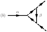
Figure 1: The first order contributions to (a) the self energy $\Sigma(\epsilon_{n})$, (b) the vertex $\Gamma_{s}(\omega_{n},\epsilon_{n})S^{\alpha}$. Solid line denotes the paramagnon propagator $D(\omega_{n})$ whereas dashed line stands for pseudofermion propagator $G(\epsilon_{n})$.

3.1 First order contributions

The corrections to the self energy $\Sigma(\epsilon_{n})$ and vertex function $\Gamma_{S}(\omega_{n},\epsilon_{n})$ of first order in $g_{0}$ are (see Fig. 1)

$$\Sigma^{(1)}(\epsilon_{n}) = J^{2}\mathbf{S}^{2}_{0}T\sum_{\omega_{s}}D(\omega_{s})G(\omega_{s}+\epsilon_{n}),$$ (10)

$$\Gamma_{S}^{(1)}(\omega_{n},\epsilon_{n}) = J^{2}\mathbf{S}^{2}_{1}T\sum_{\omega_{s}}D(\omega_{s})G(\omega_{s}+\epsilon_{n})$$ (11)

$$\hskip 36.98866pt\times G(\omega_{s}+\epsilon_{n}+\omega_{n}),$$

where $\mathbf{S}^{2}_{a}=S(S+1)-a$. Evaluation of expressions (10) and (11) at vanishing temperature yields

$$\Sigma^{(1)}(E)= - \frac{g_{0}}{2}\mathbf{S}^{2}_{0}E\ln\frac{E_{0}}{|E|},$$ (12)

$$\Gamma_{S}^{(1)}(0,E)= \frac{g_{0}}{2}\mathbf{S}^{2}_{1}\ln\frac{E_{0}}{|E|}.$$ (13)

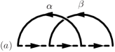
Figure 2: The second order contributions to the self energy $\Sigma(\epsilon_{n})$

3.2 Second order contributions

The second order corrections to the self energy $\Sigma$ are shown in Figs. 2(a) and 2(b) and given respectively as

$$\Sigma^{(2)}(\epsilon_{n}) = J^{4}\mathbf{S}^{2}_{0}\mathbf{S}^{2}_{1}T^{2}\sum_{\omega_{s},\omega_{m}}D(\omega_{s})D(\omega_{m})G(\omega_{s}+\epsilon_{n})$$ (14)

$$\hskip 36.98866pt\times G(\omega_{s}+\omega_{m}+\epsilon_{n})G(\omega_{m}+\epsilon_{n})$$

$$+ J^{4}\mathbf{S}^{2}_{0}\mathbf{S}^{2}_{0}T^{2}\sum_{\omega_{s},\omega_{m}}D(\omega_{s})D(\omega_{m})G^{2}(\omega_{s}+\epsilon_{n})$$

$$\hskip 36.98866pt\times G(\omega_{s}+\omega_{m}+\epsilon_{n}).$$

At $T=0$ we find

$$\Sigma^{(2)}(E)= - \frac{g^{2}_{0}}{4}\mathbf{S}^{2}_{0}\mathbf{S}^{2}_{1}E\left(\ln^{2}\frac{E_{0}}{|E|}+\ln\frac{E_{0}}{|E|}\right)$$ (15)

$$+ \frac{g_{0}^{2}}{4}\mathbf{S}^{2}_{0}\mathbf{S}^{2}_{0}E\left(\frac{1}{2}\ln^{2}\frac{E_{0}}{|E|}+\ln\frac{E_{0}}{|E|}\right).$$

The second order corrections to the vertex $\Gamma_{S}(\omega_{n},\epsilon_{n})$ are presented in Figs. 3(a)-(d). They are as follows

$$\Gamma_{s}^{(2)} = J^{4}\mathbf{S}^{2}_{1}\mathbf{S}^{2}_{2}T^{2}\sum_{\omega_{s},\omega_{m}}D(\omega_{s})G(\omega_{s}+\epsilon_{n})G(\omega_{m}+\epsilon_{n})$$ (16)

$$\times D(\omega_{m})G(\omega_{s}+\omega_{m}+\epsilon_{n})G(\omega_{s}+\omega_{m}+\epsilon_{n}+\omega_{n})$$

$$+ J^{2}\mathbf{S}^{2}_{1}T\sum_{\omega_{s}}D(\omega_{s})G(\omega_{s}+\epsilon_{n})\Gamma^{(1)}_{S}(\omega_{n},\omega_{s}+\epsilon_{n})$$

$$\hskip 28.45274pt\times G(\omega_{s}+\epsilon_{n}+\omega_{n})$$

$$+ J^{2}\mathbf{S}^{2}_{1}T\sum_{\omega_{s}}[D(\omega_{s})+D(\omega_{s}-\omega_{n})]G(\omega_{s}+\epsilon_{n})$$

$$\hskip 28.45274pt\times G^{2}(\omega_{s}+\epsilon_{n}+\omega_{n})\Sigma^{(1)}(\omega_{s}+\epsilon_{n}+\omega_{n})$$

$$+ J^{4}\mathbf{S}^{2}_{1}\mathbf{S}^{2}_{1}T^{2}\sum_{\omega_{s},\omega_{m}}D(\omega_{s})[D(\omega_{m})+D(\omega_{m}-\omega_{n})]$$

$$\hskip 28.45274pt\times G(\omega_{s}+\epsilon_{n})G(\omega_{s}+\omega_{m}+\epsilon_{n}+\omega_{n})$$

$$\hskip 28.45274pt\times G(\omega_{s}+\epsilon_{n}+\omega_{n})G(\omega_{m}+\epsilon_{n}+\omega_{n}).$$

Evaluating Eqs. (16) at $T=0$ we find

$$\Gamma_{s}^{(2)}(0,E) = \frac{g_{0}^{2}}{4}\mathbf{S}^{2}_{1}\mathbf{S}^{2}_{2}\ln\frac{E_{0}}{|E|}$$ (17)

$$+ \frac{g_{0}^{2}}{4}\mathbf{S}^{2}_{1}\mathbf{S}^{2}_{1}\left(\frac{1}{2}\ln^{2}\frac{E_{0}}{|E|}-2\ln\frac{E_{0}}{|E|}\right)$$

$$- \frac{g_{0}^{2}}{2}\mathbf{S}^{2}_{0}\mathbf{S}^{2}_{1}\left(\frac{1}{2}\ln^{2}\frac{E_{0}}{|E|}-\ln\frac{E_{0}}{|E|}\right)$$

$$+ \frac{g_{0}^{2}}{2}\mathbf{S}^{2}_{1}\mathbf{S}^{2}_{1}\left(\frac{1}{2}\ln^{2}\frac{E_{0}}{|E|}-\ln\frac{E_{0}}{|E|}\right).$$

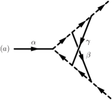
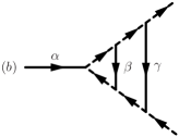
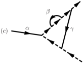
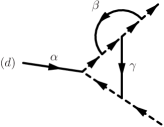
Figure 3: The second order contributions to the vertex $\Gamma_{S}(\omega_{n},\epsilon_{n})S_{\alpha}$.

3.3 Renormalization group equation for $g$

Combining together Eqs. (12), (13), (15) and (17) we obtain the following result

$$\frac{1}{g(E)}=\frac{1}{g_{0}}+\ln\frac{E_{0}}{|E|}+\alpha_{S}g_{0}\ln\frac{E_{0}}{|E|},$$ (18)

where

$$\alpha_{S}=\frac{1}{2}[(S(S+1)-1)^{2}+1].$$ (19)

We emphasize that $\ln^{2}E_{0}/|E|$ terms are cancelled out in the final expression for $1/g(E)$. Following the standard procedure IzyumovSkryabin , i.e., taking derivative of $1/g(E)$ with respect to $\xi=\ln|E|/E_{0}$ and then substituting $g(E)$ for $g_{0}$ in the right hand side of Eq. (18), we obtain the following renormalization group equation

$$\frac{dg}{d\xi}=g^{2}+\alpha_{S}g^{3}+\mathcal{O}(g^{4}).$$ (20)

Equation (20) describes the renormalization of the invariant charge $g$ in the weak coupling limit. The comparison of two first terms in the right hand side of Eq. (20) results in the inequality $g\ll\alpha_{S}^{-1}$ that determines the weak coupling limit. In virtue of the result $\alpha_{2}=13$ we find the significant reduction of the weak coupling region from a naive estimate $g\ll 1$ already for the impurity spin $S=2$.

We mention that evaluation of Eqs. (10), (11), (14) and (16) at finite temperatures but $E=0$ results in the same equation as Eq. (20) for the renormalization of $g$ with temperature but now with $\xi=\ln T/E_{0}$. This fact is in agreement with natural expectations of setting the energy scale by temperature $T$ in this case.

4 Renormalization group analysis in the strong coupling limit

In the strong coupling limit in which $g$ is assumed to be large it is convenient to use the Holstein-Primakoff representation for the impurity spin $\mathbf{S}$ HP

$$S^{+}=a^{\dagger}\sqrt{2S-a^{\dagger}a},\qquad S^{-}=\sqrt{2S-a^{\dagger}a}\,a,$$

$$S^{z}=-S+a^{\dagger}a.$$ (21)

Here $a^{\dagger}$ and $a$ denotes bosonic creation and annihilation operators. The effective action (2) becomes

$$\mathcal{S}_{\textrm{eff}}=\frac{J^{2}}{2}\int_{0}^{\beta}d\tau_{1}d\tau_{2}D(\tau_{1}-\tau_{2})\mathbf{S}(\tau_{1})\mathbf{S}(\tau_{2})$$ (22)

$$+\int_{0}^{\beta}d\tau a^{\dagger}(\tau)\partial_{\tau}a(\tau).$$

The Holstein-Primakoff representation (21) has the enlarged Hilbert space as compared with one for the spin $\mathbf{S}$. This fact becomes immaterial for $g_{0}S\gg 1$ such that we can perform expansion of the square roots in Eq. (21) in powers of $a^{\dagger}a$ and perform standard evaluation of a functional integral with the effective action (22).

Expanding the product $\mathbf{S}(\tau_{1})\mathbf{S}(\tau_{2})$ to the second order in boson fields $a^{\dagger}$ and $a$ we find the bare propagator $G(\omega_{n})$ as follows

$$G^{-1}(\omega_{n})=i\omega_{n}-\pi g_{0}S|\omega_{n}|/2.$$ (23)

The higher order in $a^{\dagger}$ and $a$ terms result in the renormalization of the $g$. At zero temperature with a help of the standard background field procedure we derive the following one-loop result

$$g(E)=g_{0}+\frac{2g}{S}\int^{E_{0}}_{-E_{0}}\frac{d\omega}{2\pi}G(\omega)\Theta(|\omega|-|E|).$$ (24)

Here $E$ plays a role of the energy scale that separates the ‘fast’ and ‘slow’ modes. After evaluation we obtain

$$g(E)=g_{0}\left[1+\frac{4}{\pi^{2}S^{2}g_{0}}\left(1-\frac{1}{1+\pi^{2}g^{2}_{0}S^{2}/4}\right)\ln\frac{|E|}{E_{0}}\right].$$ (25)

If we consider the impurity spin $\mathbf{S}$ being a classical vector of the fixed length $S$ then at zero temperature the effective action (22) is equivalent to the so-called one-dimensional $O(3)$ model with inverse square interaction. In this case the brackets in front of $\ln|E|/E_{0}$ in the right hand side of Eq. (25) should be substituted by unity due to the absence of $i\omega_{n}$ term in the propagator (23). Thus, for the $O(3)$ model each loop results in a factor $g^{-1}_{0}S^{-2}$. Additional sub-leading series in powers of $(g_{0}S)^{-1}$ appears for the action (22) as one can see from Eq. (25). Under assumption $g_{0}\gg 2/(\pi S)$ we neglect the sub-leading terms in Eq. (25). With the same accuracy in calculation of the two-loop contribution to the $g(E)$ we omit the term $i\omega_{n}$ in the propagator (23). Then, the result coincides with the two-loop result for the $O(3)$ model with inverse square interaction found in Ref. Zwerger . We obtain therefore

$$g(E)=g_{0}+\frac{4}{\pi^{2}S^{2}}\ln\frac{|E|}{E_{0}}+\frac{8}{\pi^{4}S^{4}g_{0}}\ln\frac{|E|}{E_{0}}.$$ (26)

Hence, we derive the following renormalization group equation

$$\frac{dg}{d\xi}=\frac{4}{\pi^{2}S^{2}}+\frac{8}{\pi^{4}S^{4}g}+\mathcal{O}(g^{-2}).$$ (27)

We mention that Eq. (27) coincides with the two-loop renormalization group equation known for the $O(3)$ model with inverse square interaction Zwerger . The sub-leading terms neglected above determines the condition $g\gg 2/(\pi S)$ of applicability for the strong coupling expansion.

5 Renormalization of $g$ with temperature

At relatively high temperatures $T\gtrsim E_{0}$ the invariant charge $g$ equals $g_{0}$. As temperature is lowered the $g$ starts to be renormalized. In the weak coupling regime $g\ll\alpha_{S}^{-1}$ the renormalization of $g$ with $T$ is determined by Eq. (20). If for a moment we restrict ourselves to the first term in the right hand side of Eq. (20) we find

$$g(T)=\frac{g_{0}}{1+g_{0}\ln E_{0}/T}.$$ (28)

This expression has been obtained originally by Larkin and Melnikov with a help of summation over the parquet diagrams LarkinMelnikov . Taking into account the second term in the right hand side of Eq. (20) we obtain ($T\ll T_{0}$, $g_{0}\ll\alpha_{S}^{-1}$)

$$g(T)=\left[\ln\left(\frac{T_{0}}{T}\ln^{\alpha_{S}}\frac{T_{0}}{T}\right)\right]^{-1},\quad T_{0}=g_{0}^{\alpha_{S}}e^{1/g_{0}}E_{0}.$$ (29)

Equation (29) demonstrates that for $T\ll T_{0}$ the $g(T)$ decreases as temperature is lowered faster than predicted by the lowest order result (28) and faster for larger impurity spin $S$.

In the strong coupling limit $g\gg 2/(\pi S)$ by solving Eq. (27) we find the following temperature dependence ($T\gg\tilde{T}_{0}$, $g_{0}\gg 2/(\pi S)$)

$$g(T)=\frac{4}{\pi^{2}S^{2}}\ln\left(\frac{T}{\tilde{T}_{0}}\ln^{1/2}\frac{T}{\tilde{T}_{0}}\right),$$ (30)

$$\quad\tilde{T}_{0}=\frac{\pi S\sqrt{g_{0}}}{2}e^{-\pi^{2}S^{2}g_{0}/4}E_{0}.$$

The result (30) indicates that for $T\gg\tilde{T}_{0}$ the $g(T)$ lowers with decrease of the temperature slower then logarithmically and faster for large spin $S$.

Let us now assume the existence of the renormalization group function $\phi(g)=dg/d\xi$ for all values of $g\geqslant 0$ with asymptotics given by Eqs. (20) and (27). We mention that for the impurity spin $S\leqslant 1$ Foot the weak (20) and strong (27) coupling asymptotics have a range in which they both are applicable. In the case of larger $S$ there exists a broad region $\alpha_{S}^{-1}\ll g\ll 2/(\pi S)$ where the quantitative behavior of function $\phi(g)$ is unknown. In general, it is natural to expect that the function $\phi(g)$ is positive for all $g>0$ and has the maximum at some value $g=g_{\textrm{max}}$.

Existence of the maximum in the renormalization group function $\phi(g)$ signals about the presence of a new energy scale in the problem

$$T_{\textrm{max}}=E_{0}\exp\int_{g_{0}}^{g_{\textrm{max}}}\frac{dg}{\phi(g)}.$$ (31)

For the system with large value of $g_{0}$ the energy scale $T_{\textrm{max}}$ separates temperature ranges of the strong and weak coupling regimes.

6 Susceptibility

Direct measurements of the $g(T)$ in a laboratory is impossible. Fortunately, the information about behavior of the $g(T)$ can be extracted from the zero field magnetic susceptibility of the impurity spin. By polarizing electron spins the impurity acquires a giant magnetic moment $\mu S$ with $|\mu|=\mu_{B}|g_{\textrm{imp}}-g_{e}J\nu/(1+F_{0}^{\sigma})|\gg|g_{\textrm{imp}}|\mu_{B}$. Here $\mu_{B}$ denotes the Bohr magneton, $g_{\textrm{imp}}$ and $g_{e}$ the $g$-factors of impurity and electrons respectively LarkinMelnikov ; KorenblitShender . Thus in the presence of a small magnetic field $h$ effective action (7) acquires the standard term

$$\mathcal{S}_{h}=-\mu h\int_{0}^{\beta}d\tau c^{\dagger}_{m}(\tau)S^{z}_{mm^{\prime}}c_{m^{\prime}}(\tau).$$ (32)

The zero field magnetic susceptibility of the impurity can be found as IzyumovSkryabin

$$\chi(T)=T\lim\limits_{h\to 0}\frac{\partial^{2}}{\partial h^{2}}\ln T\sum_{m,\epsilon_{n}}G_{mm}(i\epsilon_{n}).$$ (33)

It is convenient to write the general expression for the susceptibility as follows

$$\chi(T)=\frac{\mu^{2}S(S+1)}{3T}\Upsilon(g_{0},T/E_{0}).$$ (34)

Here $\Upsilon(g_{0},T/E_{0})$ is some dimensionless function and we singled out the typical factor of the Curie-Weiss susceptibility for a free spin in Eq. (34) for convenience. Let us now perform a change of the temperature scale $T\to\lambda T$ such that ZinnJustin

$$\Upsilon(g_{0},T/E_{0})=Z(\lambda)\Upsilon(g(\lambda^{-1}),\lambda T/E_{0}).$$ (35)

The conditions $Z(1)=1$ and $g(1)=g_{0}$ should be obviously imposed. The right hand side of Eq. (35) should be independent of an arbitrary scale parameter $\lambda$. Thus we obtain the following equation for $Z(\lambda)$

$$\frac{d\ln Z(\lambda)}{d\ln\lambda}=-\frac{d\ln\Upsilon(g(\lambda^{-1}),\frac{\lambda T}{E_{0}})}{d\ln\lambda}\equiv\zeta(g(\lambda^{-1})).$$ (36)

By solving Eq. (36) for $\lambda=E_{0}/T$ and taking into account that $g(T/E_{0})\equiv g(T)$ we find

$$\chi(T)=\frac{\mu^{2}S(S+1)}{3TF(g_{0})}F(g(T)),$$ (37)

where we have used the fact that $\Upsilon(g(T),1)=1$ and

$$F(g)=\exp\left(-\int_{g_{\textrm{max}}}^{g}du\frac{\zeta(u)}{\phi(u)}\right).$$ (38)

In the weak coupling regime we compute $\Upsilon(g(\frac{1}{\lambda}),\frac{\lambda T}{E_{0}})$ perturbatively in $g(\lambda^{-1})$ for $\lambda$ of the order of $E_{0}/T$. To the lowest order in $g(\lambda^{-1})$ the pseudofermion Green function in the presence of a small magnetic field $h$ becomes

$$G^{-1}_{mm^{\prime}}(\epsilon_{n})=\delta_{mm^{\prime}}\left[(i\epsilon_{n}+\eta)\Gamma(\epsilon_{n})-hm\Gamma_{S}(0,\epsilon_{n})\right].$$ (39)

Here $\Gamma(\epsilon_{n})$ and $\Gamma_{S}(0,\epsilon_{n})$ are given by Eqs. (12) and (13). With a help of Eq. (33) we find

$$\Upsilon(g(\lambda^{-1}),\lambda T/E_{0})=1+g(\lambda^{-1})\ln\frac{\lambda T}{E_{0}}.$$ (40)

Then Eq. (40) yields

$$\zeta(g)=-g-\mathcal{O}(g^{2})$$ (41)

and we obtain the function $F(g)$ at $g\ll\alpha_{S}^{-1}$ as

$$F(g)=\textrm{const}\,g(1+\mathcal{O}(g)).$$ (42)

Equations (40) and (42) allow us to derive the following result for the susceptibility $\chi(T)$ in the weak coupling regime, $g\ll\alpha_{S}^{-1}$,

$$\chi(T)=\frac{\mu^{2}S(S+1)g(T)}{3Tg_{0}}.$$ (43)

We mention that the result (43) with $g(T)$ given by Eq. (28) was first found by Larkin and Melnikov LarkinMelnikov with a help of a direct summation of the parquet diagrams. The derivation presented above is more general since the true invariant charge $g(T)$ enters into Eq. (43). With a help of Eq. (43) we find the temperature behavior of the susceptibility $\chi(T)$ at $T\ll T_{0}$ ($g_{0}\ll\alpha_{S}^{-1}$) as follows

$$\chi(T)=\frac{\mu^{2}S(S+1)}{3Tg_{0}}\left[\ln\left(\frac{T_{0}}{T}\ln^{\alpha_{S}}\frac{T_{0}}{T}\right)\right]^{-1}.$$ (44)

In the strong coupling limit we can perform similar analysis as above by expansion in powers of $1/g(\lambda^{-1})$ when $\lambda$ is of the order of $E_{0}/T$. By using the perturbative result

$$\Upsilon(g(\lambda^{-1}),\lambda T/E_{0})=1+\frac{4}{\pi^{2}S(S+1)g(\lambda^{-1})}\ln\frac{\lambda T}{E_{0}}$$ (45)

we obtain

$$\zeta(g)=-\frac{4}{\pi^{2}S(S+1)g}+\mathcal{O}(g^{-2}).$$ (46)

Hence, we find

$$F(g)=\textrm{const}\,g^{S/(S+1)}(1+\mathcal{O}(g^{-1})).$$ (47)

With a help of Eqs (45) and (47) we derive the following result for the susceptibility $\chi(T)$ in the strong coupling regime, $g\gg 2/(\pi S)$,

$$\chi(T)=\frac{\mu^{2}S(S+1)}{3T}\left[\frac{g(T)}{g_{0}}\right]^{S/(S+1)}.$$ (48)

By using Eq. (30), we obtain the temperature behavior of the susceptibility at $T\gg\tilde{T}_{0}$ ($g_{0}\gg 2/(\pi S)$) as follows

$$\chi(T)=\frac{\mu^{2}S(S+1)}{3Tg_{0}^{S/(S+1)}}\left[\frac{4}{\pi^{2}S^{2}}\ln\left(\frac{T}{\tilde{T}_{0}}\ln^{1/2}\frac{T}{\tilde{T}_{0}}\right)\right]^{S/(S+1)}.$$ (49)

It is worthwhile to mention that for $S\gg 1$ when the impurity spin becomes classical the function $T\chi(T)$ is proportional to $g(T)$ in both weak and strong coupling regimes.

According to Eqs. (43) and (48) the quantity $T\chi(T)$ decreases with lowering temperature. The derivative $Td(T\chi(T))/dT$ should have the maximum at some intermediate temperature $T_{\star}$ that determines by the condition $\zeta^{2}(g)=\phi(g)\zeta^{\prime}(g)$. We mention that in general the $T_{\star}$ does not coincide with the energy scale $T_{\textrm{max}}$. We present sketches for the temperature behavior of the functions $T\chi(T)$ and $Td(T\chi(T))/dT$ in Fig. 4.

Figure 4: Sketch for dependencies of the functions $T\chi(T)$ (solid curve) and $Td(T\chi(T))/dT$ (dashed curve) on $\ln T/T_{\star}$. Both curves are obtained by interpolation between the weak (43) and strong (48) coupling asymptotics. See text.

7 Conclusions

In conclusions we performed the renormalization group analysis for the problem of the magnetic impurity in nearly ferromagnetic Fermi liquid. We evaluated the second order term in the weak coupling expansion of the renormalization group equation for the invariant charge $g$. We derived the two-loop renormalization group equation for the $g$ in the strong coupling regime. We found the low and high temperature asymptotics of the magnetic susceptibility of the impurity spin $\chi(T)$ and showed that the derivative $Td(T\chi(T))/dT$ has the maximum.

In the discussion above we have neglected the usual Kondo contributions Kondo ; IzyumovSkryabin which involve odd powers of $J\nu$. However such terms do not contain the anomalously large coefficients $(1+F_{0}^{\sigma})^{-1}$ as it occurs in terms of even powers considered above. As it was originally shown by Larkin and Melnikov LarkinMelnikov the condition $g\gg|J|\nu$, or equivalently, $|J|\nu\gg 1+F_{0}^{\sigma}$ is sufficient to omit odd in $J\nu$ terms. The results obtained above are valid therefore only at not too low temperatures $T\gg T_{l}=E_{0}\exp[-c(1+F_{0}^{\sigma})^{-1}]$ where $c=1/(16a^{2}p_{F}^{2})$. For $c$ of the order of unity and $1+F_{0}^{\sigma}\ll 1$ the temperature $T_{l}$ can be of the several orders in magnitude less than $E_{0}$. At the temperature $T_{l}$ the giant magnetic moment of the impurity $\mu$ is totally compensated such that the impurity susceptibility becomes $\chi(T_{l})\sim\mu_{B}^{2}S(S+1)/T_{l}$. At lower temperatures $T\lesssim T_{l}$ the usual physics of the multichannel Kondo problem MultiKondo with the number of channels of the order of $c(1+F_{0}^{\sigma})^{-1}$ manifests. It is worthwhile to mention that the presence of the paramagnons complicates the subject as compared with the standard multichannel Kondo problem at $T\lesssim T_{l}$ Maebashi .

Also we mention that the temperature dependence of part of the resistance related with scattering on the magnetic impurities should have the same features as quantity $T\chi(T)$ for not too low temperatures $T\gg T_{l}$ LarkinMelnikov .

Finally, we emphasize that new detailed experimental investigations of the zero field magnetic susceptibility of impurity as well as the resistance in nearly ferromagnetic Fermi liquid are necessary to test the predictions made in the paper.

References

(1) see, e.g.,
B. N. Narozhny, I. L. Aleiner and A. I. Larkin, Phys. Rev.
B 62, 14898 (2000); A. J. Millis, D. K. Morr, and
J. Schmalian, Phys. Rev. Lett. 87, 167202 (2001);
M. A. Skvortsov, A. I. Larkin and M. V. Feigelman, Phys.
Rev. Lett. 92, 247002 (2004)
(2) E. C. Stoner Rep. Prog. Phys. 11, 43
(1947); I. Ya. Pomeranchuk, Zh. Éksp. Teor. Fiz.
35, 524 (1958) [Sov. Phys. JETP 8, 524 (1959)]
(3) J. Kondo, Prog. Theor. Phys. 32, 37
(1964)
(4) A. M. Tsvelik and P. B. Wiegmann, Adv. of
Phys. 32, 453 (1983); N. Andrei, K. Furuya, and
J. H. Lowenstein, Rev. Mod. Phys. 55, 331 (1983)
(5) A. I. Larkin and V. I. Melnikov,
Sov. Phys. JETP 34, 656 (1972) [Zh. Éksp. Teor. Fiz.
61, 1232 (1971)]
(6) A. A. Abrikosov, L. P. Gor’kov, I. E. Dzyaloshinksky,
Methods of quantum field theory in statistical physics,
(Prentice Hall, Englewood Cliffs, N.J., 1963)
(7) S. Doniachand S. Engelsberg, Phys.
Rev. Lett. 17, 750 (1966)
(8) R. M. Bozorth, P. A. Wolff, D. D. Davis, and
J. H. Wernick, Phys. Rev. 122, 1157 (1961);
A. M. Clogston, B. T. Matthias, M. Peter, H. J. Williams,
E. Corenswit, and R. C. Sherwood, Phys. Rev. 125, 541
(1962); D. Shaltiel, J. H. Wrenick, and H. J. Williams, Phys.
Rev. 135, A1346, (1964); L. Shen, D. S. Schreiber, and
A. J. Arko, Phys. Rev. 179, 512 (1969)
(9) For a review, see I. Ya. Korenblit and E. F. Shender,
Usp. Fiz. Nauk 126, 233 (1978)
(10) H. Beckmann and G. Bergmann, Phys. Rev.
Lett. 83, 2417 (2000); G. Bergmann and M. Hossain,
Phys. Rev. Lett. 86 2138 (2001)
(11) A. I. Larkin and V. I. Melnikov, JETP Lett. 20, 172
1974 [Pis’ma Zh. Éksp. Teor. Fiz. 20, 386 (1974)];
A. M. Dyugaev, JETP Lett. 23, 138 (1976) [Pis’ma Zh.
Éksp. Teor. Fiz. 23, 156 (1976)]
(12) In general, there are higher order terms in
the series expansion of the
in powers of
. If we take the term proportional
into account then we find that
for and at
(13) R. L. Stratonovich, Dokl. Akad. Nauk SSSR 2, 1097
(1957) [Sov. Phys. Doklady 2, 416 (1957)]; J. Hubbard,
Phys. Rev. Lett. 3, 77 (1959)
(14) A. A. Abrikosov, Physics 2, 21
(1965)
(15) see, e.g., Yu. A. Izyumov and Yu. N. Skryabin,
Statistical mechanics of magnetoordered systems, (Moskva,
Nauka, 1987) (in russian)
(16) see, e.g.,
N. N. Bogolubov an D. V. Shirkov, Introduction to the
theory of quantized fields, Interscience, London (1959)
(17) For a different propagator similar
second order diagrams were analysed recently in
A. V. Syromyatnikov and S. V. Maleev, Phys. Rev. B
72, 174419 (2005)
(18) T. Holstein and H. Primakoff, Phys. Rev.
58, 1098 (1940).
(19) W. Hofstetter and W. Zwerger, Phys. Rev. Lett.
78, 3737 (1997); Eur. Phys. J. B 5, 751 (1998);
the parameter used by authors equals in our
notations
(20) For Ni atom spin , for Co atom and for Fe atom
(21) see, e.g., J. Zinn-Justin,
Quantum Field Theory and Critical Phenomena, (Clarendon Press,
Oxford, 1993)
(22) P. Nozières and A. Blandin, J. Phys.
(France) 41, 193 (1980); A. M. Tsvelik and
P. B. Wiegmann, Z. Phys. B 54, 201 (1984); N. Andrei
and C. Destri, Phys. Rev. Lett. 52, 364 (1984)
(23) H. Maebashi, K. Miyake, and C. M. Varma,
Phys. Rev. Lett. 88, 226403 (2002)