Gauge field for edge state in graphene

Abstract

By considering the continuous model for graphene, we analytically study a special gauge field for the edge state. The gauge field explains the properties of the edge state such as the existence only on the zigzag edge, the partial appearance in the $k$-space, and the energy position around the Fermi energy. It is demonstrated utilizing the gauge field that the edge state is robust for surface reconstruction, and the next nearest-neighbor interaction which breaks the particle-hole symmetry stabilizes the edge state.

1 Introduction

A single layer of graphite or graphene is an element of various carbon-based materials such as carbon nanotubes. [1] These materials are eminently suitable for future nanotechnology and thus fundamental understanding of the electronic properties is indispensable. The electronic property of graphene is mainly determined by the $\pi$-electrons around the Fermi energy at the hexagonal corners (the K and K^′ points) of the two-dimensional Brillouin zone. It is known that the eigenstates are classified into extended states and localized states. The edge state existing near the zigzag edge is an example of the localized state. [2] The tight-binding (TB) lattice model has shown that the edge state exists near the zigzag edge while no localized state exists near the armchair edge. [2, 3] Recently, by scanning tunneling microscopy and spectroscopy (STM/STS) experiments, Niimi et al. [4] and Kobayashi et al. [5], respectively, observed the edge state near the zigzag edge and the energy position.

The edge shape determines the boundary condition for the wave function. It has been shown in the studies of single-walled carbon nanotubes (SWNTs) that a boundary condition can be changed by an external magnetic field and uniform lattice deformations. Using the continuous model of graphene, [6] Ajiki and Ando [7] showed that a uniform magnetic field parallel to a SWNT axis affects the energy band structure of extended states. The magnetic field is expressed by a gauge field which changes the boundary condition around a tube axis through the Aharonov-Bohm (AB) effect. Zaric et al. [8] observed optical signatures of the AB effect. Kane and Mele [9] introduced another homogeneous gauge field in the continuous model. The gauge field represents uniform lattice deformations such as uniform bend, twist and curvature. The gauge field changes the boundary condition around a tube axis through a generalized AB effect and makes a mini gap in chiral metallic SWNTs. The curvature-induced mini gap was observed by STS experiment by Ouyang et al. [10] The perturbations above modify the boundary condition for extended states and are similar in that they are represented by gauge fields in the continuous model. Is it possible to change the boundary condition for the edge state? To answer this question, a generalization of the gauge fields to local fields is necessary since the edge states appear locally around the edge. In the previous paper, [11] we generalize the gauge field introduced by Kane and Mele, to include a local lattice deformation of graphene. The deformation-induced gauge field accounts for the local modulation of the energy band gap, [11] which was observed in some pea-pod-like structures by Lee et al. [12] In this paper, using the continuous model, we show that the edge state can be formed by a deformation-induced “magnetic” field and we clarify why the edge state is formed in the zigzag edge, but not in the armchair edge. We explain various properties of the edge states, and examine how the edge state are affected by perturbations.

Here we briefly introduce the continuous model. In an undeformed graphene, the Hamiltonian for $\pi$-electrons around the Fermi point are given by two-component Weyl equation. [6] Two components of the wave function represent the two sublattices in the unit cell. The Weyl equation gives two-dimensional linear $k$ energy dispersion relation around the K and K^′ points in the Brillouin zone. The Weyl equation allows us to treat a variety of perturbations in a unified way for studying transport properties, scattering process around impurities, lattice defects and topological defects. [13]

This paper is organized as follows. In § 2, we define a gauge field for a locally deformed graphene system. Then we solve the continuous model (Weyl equation with the gauge field) to obtain the edge state. In § 3, we present several applications of the continuous model. The effects of a lattice deformation around the edge, the next nearest-neighbor interaction, and an external magnetic field on the edge state are examined. In § 4, we discuss and summarize the results. We derive the continuous model in Appendix A. In Appendix B, we analyze a locally deformed graphene system using the TB model.

2 Continuous Model

We consider an undeformed graphene as shown in Fig. 1(a). The unit cell consists of A sublattice ($\bullet$) and B sublattice ($\circ$), and each sublattice is spanned by primitive vectors $\mathbf{a}_{1}$ and $\mathbf{a}_{2}$. $|2\mathbf{a}_{2}-\mathbf{a}_{1}|\equiv 2\ell$ is the unit length along the $y$-axis. A $\pi$-electron hops from one site to the nearest-neighbor sites with the hopping integral $-\gamma_{0}$ ($\approx-3$ eV) in each hopping process. Let $v_{F}(\equiv\gamma_{0}\ell/\hbar)$ be the Fermi velocity and $\hat{\mathbf{p}}\equiv(\hat{p}_{x},\hat{p}_{y})$ the momentum operator. The Hamiltonian for $\pi$-electrons around the K point is then written as [6]

$${\cal H}_{\rm K}^{0}=v_{F}\mbox{\boldmath$\sigma$}^{\prime}\cdot\hat{\bf{p}}=v_{F}\begin{pmatrix}0&-\hat{p}_{x}-i\hat{p}_{y}\cr-\hat{p}_{x}+i\hat{p}_{y}&0\end{pmatrix},$$ (1)

where $\mbox{\boldmath$\sigma$}^{\prime}\equiv(-\sigma_{x},\sigma_{y})$ and $\sigma_{i}$ ($i=x,y,z$) are the Pauli matrices. The Hamiltonian operates on a two-component wave function $\psi^{\rm K}({\mathbf{r}})={}^{t}(\psi^{\rm K}_{\rm A}({\bf r}),\psi^{\rm K}_{\rm B}({\bf r}))$. This two-component character is referred to as the pseudo-spin; hence, $\psi_{\rm A}^{\rm K}({\bf r})$ and $\psi^{\rm K}_{\rm B}({\bf r})$ are the pseudo-spin up and down states, respectively. The energy eigenequation ${\cal H}_{\rm K}^{0}\psi_{E}^{\rm K}({\mathbf{r}})=E\psi_{E}^{\rm K}({\mathbf{r}})$ is the Weyl equation.

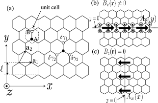
Figure 1: (a) Lattice structure of graphene. The unit cell consists of A (closed circle) and B (open circle) sublattices, which leads to the pseudo-spin structure of the wave function. Local modulations of the hopping integral is defined by $\delta\gamma_{a}(\mathbf{r})$ ($a=1,2,3$). Two examples of local deformation (borders) and resultant deformation-induced gauge fields are shown in (b) and (c). In (b), the gauge field (arrows) gives a finite deformation-induced magnetic field (flux) illustrated by $\odot$ and $\otimes$ while no deformation-induced magnetic field is present in (c).

When the lattice is deformed locally, the nearest-neighbor hopping integral depends on the position as $-\gamma_{0}+\delta\gamma_{a}(\mathbf{r})$ ($a=1,2,3$) where $a$ denotes three nearest-neighbor B sites from an A atom (see Fig. 1(a)). The Hamiltonian can be expressed by

$${\cal H}_{\rm K}=v_{F}\mbox{\boldmath$\sigma$}^{\prime}\cdot(\hat{\bf{p}}-\bf{A}({\bf r})),$$ (2)

where the vector field $\mathbf{A}(\mathbf{r})=(A_{x}(\mathbf{r}),A_{y}(\mathbf{r}))$ is the deformation-induced gauge field. For a weak lattice deformation satisfying $|\delta\gamma_{a}(\mathbf{r})|\ll\gamma_{0}$, the gauge field is expressed by a linear combination of $\delta\gamma_{a}(\mathbf{r})$ as [11] (see Appendix A)

$$\begin{split}&v_{F}A_{x}({\bf r})=\delta\gamma_{1}({\bf r})-\frac{1}{2}\left(\delta\gamma_{2}({\bf r})+\delta\gamma_{3}({\bf r})\right),\\ &v_{F}A_{y}({\bf r})=\frac{\sqrt{3}}{2}\left(\delta\gamma_{2}({\bf r})-\delta\gamma_{3}({\bf r})\right).\end{split}$$ (3)

Here, we give two examples of local lattice deformation on a line (Figs. 1(b) and 1(c)). From now we call this type of lattice deformation border. The example of Fig. 1(b) is a modification of C-C bond lengths in a row at $y=0$, namely, $\delta\gamma_{1}(\mathbf{r})\neq 0$ at $y=0$ and $\delta\gamma_{2}(\mathbf{r})=\delta\gamma_{3}(\mathbf{r})=0$. From eq.(3), we obtain $v_{F}\mathbf{A}(y)=(\delta\gamma_{1}(y),0)$. The example of Fig. 1(c) is that $\delta\gamma_{1}(\mathbf{r})=0$ and $\delta\gamma_{2}(\mathbf{r})=\delta\gamma_{3}(\mathbf{r})\neq 0$ at $x=0$. We obtain $v_{F}\mathbf{A}(x)=(-\delta\gamma_{2}(x),0)$ for this case. Figures 1(b) and 1(c) correspond to the zigzag edge and the armchair edge if we take $\delta\gamma_{1}=\gamma_{0}$ and $\delta\gamma_{2}=\delta\gamma_{3}=\gamma_{0}$, respectively. The difference between the two gauge fields becomes clear by defining the deformation-induced “magnetic” field,

$$B_{z}(\mathbf{r})\equiv\frac{\partial A_{y}(\mathbf{r})}{\partial x}-\frac{\partial A_{x}(\mathbf{r})}{\partial y},$$ (4)

which is perpendicular to the graphene plane ${\bf B}(\mathbf{r})=(0,0,B_{z}(\mathbf{r}))$. It should be noted that it is not a real magnetic field. It is called a magnetic field only because it enters the Hamiltonian in the similar way as the real magnetic field. We have a finite deformation-induced magnetic field for Fig. 1(b), and zero magnetic field for Fig. 1(c). The gauge field which gives zero magnetic field can be removed from eq.(2) by a gauge transformation. [11] As shown in Fig. 1(b), the magnetic field appears locally around $y=0$; $B_{z}(y)$ is negative at $y<0$ as illustrated by $\otimes$ and is positive at $y>0$ as $\odot$. The deformation-induced magnetic field will account for the presence of edge states not at the armchair edge but at the zigzag edge. The importance of the magnetic field can be seen by the fact that the energy eigenstate of eq.(2) also satisfies ${\cal H}_{\rm K}^{2}\psi^{\rm K}_{E}(\mathbf{r})=E^{2}\psi^{\rm K}_{E}(\mathbf{r})$:

$$v_{F}^{2}\left\{(\hat{\mathbf{p}}-\mathbf{A}(\mathbf{r}))^{2}+\hbar B_{z}(\mathbf{r})\sigma_{z}\right\}\psi^{\rm K}_{E}(\mathbf{r})=E^{2}\psi^{\rm K}_{E}(\mathbf{r}).$$ (5)

${\cal H}_{\rm K}^{2}$ has only diagonal-components in the 2$\times$2 matrix. One can see that $B_{z}(\mathbf{r})$ in eq.(5) works as a potential and affects the electronic properties. This is because the diagonal element is similar to the non-relativistic Hamiltonian ${\cal H}_{\rm nr}=(1/2m)(\hat{\bf{p}}-\mathbf{A}(\mathbf{r}))^{2}\pm V(\mathbf{r})$ where the sign in front of $V(\mathbf{r})$ corresponds to the pseudo-spin and $m$ is a mass.

We derive the edge states from the Weyl equation with the gauge field of Fig. 1(b), corresponding to the zigzag edge. Before going into detail, we outline the results here. We will show that there are localized states in the energy spectrum and the energy dispersion appears as the two solid lines at $p_{x}>0$ shown in Fig. 2(b). The velocity becomes small with increasing the gauge field and it becomes zero when the gauge field is sufficiently strong. The result of the continuous model reproduces the flat band of the edge states shown in Fig. 2(e) which is calculated from the TB model [2] with the zigzag edge.

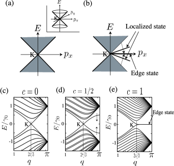
Figure 2: (a) Band structure $(p_{x},E)$ around the K point of the Weyl equation without the deformation-induced gauge field and (b) that with the gauge field at the border. The shaded regions in (a) and (b) represent the spectrum of extended states. The (two-dimensional) dispersion relation around the K point for graphene without the border gives two cones (representing the linear $k$ dispersion) whose apex is the K point as is shown in the inset of (a). The band structure of (a) is a one-dimensional projection (onto $p_{y}$ plane) of the linear $k$ dispersion. In (b), the energy dispersion for the localized state is represented by solid lines. When the bonds at $y=0$ become disconnected and zigzag edges appear, the energy eigenvalues of the localized state converge to zero ($E\to 0$) for any $p_{x}(>0)$ and forms a flat energy band of edge state. Using the TB model, we plot the band structure for an undeformed graphene in (c), for a zigzag ribbon in (e), and for a graphene with the border (with weakened hopping for the C-C bonds at $y=0$) in (d). $q$ in (c), (d) and (e) is the momentum parallel to the border and $q=2\pi/3$ is the K point.

We assume that $\mathbf{A}(\mathbf{r})$ of Fig. 1(b) is quite localized within $|y|<\xi_{g}$ where $\xi_{g}$ is a length of the order of lattice spacing, namely, $\mathbf{A}(\mathbf{r})=(A_{x}(y),0)$ and $A_{x}(y)=0$ for $|y|\geq\xi_{g}$ in eq.(2). We parameterize the localized energy eigenstate as

$$\psi^{\rm K}_{E}(\mathbf{r})=N^{\prime}\exp(i\frac{p_{x}x}{\hbar})e^{-G(y)}\begin{pmatrix}e^{+g(y)}\cr e^{-g(y)}\end{pmatrix},$$ (6)

where $N^{\prime}$ is a normalization constant. The pseudo-spin modulation is represented by $g(y)$, and the wave vector $p_{x}$ is a good quantum number because of the translational symmetry along the border. Putting eq.(6) to the energy eigenequation, ${\cal H}_{\rm K}\psi^{\rm K}_{E}(\mathbf{r})=E\psi^{\rm K}_{E}(\mathbf{r})$, we obtain

$$\begin{split}&p_{x}-A_{x}(y)-\hbar\frac{d}{dy}\left(G(y)+g(y)\right)=-\frac{E}{v_{F}}e^{+2g(y)},\\ &p_{x}-A_{x}(y)+\hbar\frac{d}{dy}\left(G(y)-g(y))\right)=-\frac{E}{v_{F}}e^{-2g(y)}.\end{split}$$ (7)

By summing and subtracting the both sides of eq.(7), we rewrite the energy eigenequation as

$$\begin{split}&p_{x}-A_{x}(y)-\hbar\frac{dg(y)}{dy}=-\frac{E}{v_{F}}\cosh(2g(y)),\\ &\hbar\frac{dG(y)}{dy}=\frac{E}{v_{F}}\sinh(2g(y)).\end{split}$$ (8)

Since we are considering a localized solution around the border, we assume $G(y)\sim|y|/\xi$ where $\xi$ $(>0)$ is the localization length. When $G(y)\sim|y|/\xi$, the solution of the second equation of eq.(8) is given by

$$g(y)=\left\{\begin{array}[]{@{\,}ll}-\frac{1}{2}\sinh^{-1}\left(\frac{\hbar v_{F}}{\xi E}\right)&(y\leq-\xi_{g}),\\ +\frac{1}{2}\sinh^{-1}\left(\frac{\hbar v_{F}}{\xi E}\right)&(y\geq\xi_{g}).\end{array}\right.$$ (11)

The functions $G(y)$ and $g(y)$ are schematically shown in Fig. 3(a) and 3(b), respectively. The sign of $g(y)$ changes across the border; this sign change means that the pseudo-spin flips at the border. The flip is induced by the gauge field $A_{x}(y)$. To see this, we integrate the first equation of eq.(8) from $y=-\xi_{g}$ to $\xi_{g}$, and acquire

$$-\int_{-\xi_{g}}^{\xi_{g}}\frac{dg(y)}{dy}dy=\frac{1}{\hbar}\int_{-\xi_{g}}^{\xi_{g}}A_{x}(y)dy.$$ (12)

We have neglected other terms, since they are proportional to $\xi_{g}$ and become zero in the limit of $\xi_{g}=0$. By putting eq.(11) to eq.(12), we find

$$-\sinh^{-1}\left(\frac{\hbar v_{F}}{\xi E}\right)=\frac{1}{\hbar}\int_{-\xi_{g}}^{\xi_{g}}A_{x}(y)dy.$$ (13)

When the right-hand side of eq.(13) is large, one obtain from eq.(11) that $g(y)\gg 0$ for $y\leq-\xi_{g}$ and $g(y)\ll 0$ for $y\geq\xi_{g}$. In this case, the localized state is approximately a pseudo-spin-up state $\psi^{\rm K}_{E}(\mathbf{r})\propto{}^{t}(1,0)$ for $y\leq-\xi_{g}$ and a pseudo-spin-down state $\psi^{\rm K}_{E}(\mathbf{r})\propto{}^{t}(0,1)$ for $y\geq\xi_{g}$. Hence, a strong gauge field at the border makes pseudo-spin-polarized localized states. Since the polarization of the pseudo-spin means that the wave function has amplitude only A (or B) sublattice, this result agrees with the result by the TB model for the edge state. [2]

Figure 3: (a) The amplitude of the wave function, $\exp(-G(y))$, of a localized state whose localization length is $\xi$. (b) The pseudo-spin modulation part, $g(y)$. From eq.(11), $g(y)$ is a constant for $|y|\geq\xi_{g}$, and abruptly changes across the border ($y=0$).

Having described the wave function of the localized state, let us now calculate $E$ and $\xi$. To this end, we use the first equation of eq.(8) for $|y|\geq\xi_{g}$ and obtain

$$\frac{E}{v_{F}}=\frac{-p_{x}}{\cosh\left(\displaystyle\frac{1}{\hbar}\int_{-\xi_{g}}^{\xi_{g}}A_{x}(y)dy\right)}.$$ (14)

Moreover, using eq.(13), we find

$$\frac{\hbar}{\xi}=p_{x}\tanh\left(\displaystyle\frac{1}{\hbar}\int_{-\xi_{g}}^{\xi_{g}}A_{x}(y)dy\right).$$ (15)

In addition to this localized state, there is another localized state for the same $p_{x}$ with the same $\xi$ but with an opposite sign of $E$. This results from a particle-hole symmetry of the Hamiltonian; $\sigma_{z}{\cal H}_{\rm K}\sigma_{z}=-{\cal H}_{\rm K}$. By the particle-hole symmetry operation, the wave function is transformed as $\psi^{\rm K}_{-E}(\mathbf{r})=\sigma_{z}\psi^{\rm K}_{E}(\mathbf{r})$.

The normalization condition of the wave function requires that $\xi$ should be positive, which restricts the value of $p_{x}$ in eq.(15). Indeed, when $A_{x}(y)$ is positive, eq.(15) means that the localized states appear only at $p_{x}>0$ around the K point. This is the reason why the localized states appear in the energy spectrum only in one side around the K point in Fig. 2(b). On the other hand, the Hamiltonian around the K^′ point is expressed by

$${\cal H}_{\rm K^{\prime}}=v_{F}\mbox{\boldmath$\sigma$}\cdot(\hat{\mathbf{p}}+\mathbf{A}(\mathbf{r})),$$ (16)

where $\mbox{\boldmath$\sigma$}\equiv(\sigma_{x},\sigma_{y})$. The different signs in front of $\mathbf{A}(\mathbf{r})$ in eqs.(2) and (16) guarantee the time-reversal symmetry. Because of the different signs, a similar argument as we used for the K point concludes that the localized state appears $p_{x}<0$ around the K^′ point. Furthermore, when $(1/\hbar)\int_{-\xi_{g}}^{\xi_{g}}A_{x}(y)dy\gg 0$, $E$ in eq.(14) becomes zero. The zero energy eigenvalue between the K and K^′ points in the band structure corresponds to the flat energy band of the edge state. [2]

When $A_{x}(y)$ is negative ($A_{x}(y)\ll 0$), a flat energy band appears in the opposite side: $p_{x}<0$ around the K point and $p_{x}>0$ around the K^′ point. This condition, $A_{x}(y)\ll 0$, corresponds to the Klein’s edges [14] which are obtained by removing A or B sites out of the zigzag edges having A or B sites. Calculations on the TB model with the Klein’s edges [14] also agree with these results obtained here.

There are also extended states in addition to the edge states. The energy dispersion relation of extended states can be obtained as $(E/v_{F})^{2}=p_{x}^{2}+p_{y}^{2}$, by setting $G(y)\sim-ip_{y}y/\hbar$ ($|y|\geq\xi_{g}$) in eqs.(6) and (8) where $p_{y}$ is a real number. The calculated energy bands are given by $|E|>v_{F}|p_{x}|$, shown as a shaded region in Fig. 2(b). It also agrees with the TB calculation shown in Fig. 2(e). One can then regard the localized state as a state with a complex wavenumber as follows. Since $1-\tanh^{2}x=1/\cosh^{2}x$, we see that the energy dispersion relation of the localized state between $E$ and $\xi$ becomes

$$\left(\frac{E}{v_{F}}\right)^{2}=p_{x}^{2}-\left(\frac{\hbar}{\xi}\right)^{2},\ \ (|y|\geq\xi_{g}),$$ (17)

which is the same as the linear dispersion relation $(E/v_{F})^{2}=p_{x}^{2}+p_{y}^{2}$ if one replaces $p_{y}$ with $i(\hbar/\xi)$.

We have shown that three basic properties of the edge states, i.e., the pseudo-spin polarization, the dependence on the momentum, and the flat energy band, obtained previously by the TB model, [2] can be explained in terms of the gauge field. In order to quantitatively compare the present theory with the TB model, we have performed a TB calculation for the geometry of Fig. 1(b) with changing $\delta\gamma_{1}$. Here, we introduce an adiabatic parameter $c$ by $\delta\gamma_{1}=c\gamma_{0}$, that is, $c=0$ and $c=1$ correspond to no deformation and the zigzag edge, respectively. In Figs. 2(c), 2(d) and 2(e), we plot the band structure for $c=0$, $c=1/2$, and $c=1$. Comparing these figures with the results of the continuous model, one can find a good correspondence between the TB model and continuous model. Moreover, we analytically find (see Appendix B)

$$\begin{split}&\frac{|E|}{v_{F}}=\frac{|p_{x}|}{\cosh(-\ln(1-c))}+{\cal O}(lp_{x}^{2}/\hbar),\\ &\frac{\hbar}{\xi}=p_{x}\tanh(-\ln(1-c))+{\cal O}(lp_{x}^{2}/\hbar),\end{split}$$ (18)

for localized states around the K point. Thus, by comparing eq.(18) with eqs.(14) and (15), we conclude that the TB model and the continuous model agree with each other near the K point ($p_{x}l/\hbar\ll 1$), by the following relationship

$$\frac{1}{\hbar}\int_{-\xi_{g}}^{\xi_{g}}A_{x}(y)dy=-\ln(1-c).$$ (19)

The right-hand side diverges when $c\to 1$, which reproduces the flat energy band ($E\to 0$) in eq.(14) and gives $\xi/\hbar=p_{x}^{-1}$ in eq.(15).

When a deformed graphene is located in an external magnetic field, the Hamiltonians for the K and K^′ points are given by replacing $\hat{\mathbf{p}}$ in eqs.(2) and (16) with $\hat{\mathbf{p}}-e\mathbf{A}^{\rm em}(\mathbf{r})$ as

$$\begin{split}&{\cal H}_{\rm K}=v_{F}\mbox{\boldmath$\sigma$}^{\prime}\cdot(\hat{\mathbf{p}}-e\mathbf{A}^{\rm em}(\mathbf{r})-\mathbf{A}(\mathbf{r})),\\ &{\cal H}_{\rm K^{\prime}}=v_{F}\mbox{\boldmath$\sigma$}\cdot(\hat{\mathbf{p}}-e\mathbf{A}^{\rm em}(\mathbf{r})+\mathbf{A}(\mathbf{r})),\end{split}$$ (20)

where $e$ denotes the electron charge and $\mathbf{A}^{\rm em}(\mathbf{r})$ is the gauge field for the external magnetic field. The $z$-component of the external magnetic field is given by

$$B_{z}^{\rm em}(\mathbf{r})\equiv\frac{\partial A_{y}^{\rm em}(\mathbf{r})}{\partial x}-\frac{\partial A_{x}^{\rm em}(\mathbf{r})}{\partial y}.$$ (21)

The same signs in front of $e\mathbf{A}^{\rm em}(\mathbf{r})$ in eq.(20) reflect the violation of time-reversal symmetry. Due to the similarity between the external magnetic field and the deformation-induced magnetic field in eq. (20), one may expect that the edge states can be induced also by $\mathbf{A}^{\rm em}(\mathbf{r})$. However, as we will see in § 3, the deformation-induced magnetic field for the edge state corresponds approximately to one flux quantum in a hexagonal unit cell, and is thus extremely strong ($\sim 10^{5}$ T), compared with the external magnetic field.

3 Application of Continuous Model

In this section, we apply the continuous model to the following three examples.

First, we consider an effect of surface reconstruction (SR) around the zigzag edge on the edge state. Since the SR is an additional lattice deformation around the edge, it can be expressed by an additional gauge field in the continuous model. Let $\delta\mathbf{A}^{\rm SR}(\mathbf{r})=(\delta A^{\rm SR}_{x},\delta A^{\rm SR}_{y})$ be the gauge field for SR. The perturbation is then represented by

$$\delta{\cal H}^{\rm SR}(\mathbf{r})=v_{F}\begin{pmatrix}0&\delta A^{\rm SR}_{x}+i\delta A^{\rm SR}_{y}\cr\delta A^{\rm SR}_{x}-i\delta A^{\rm SR}_{y}&0\end{pmatrix}.$$ (22)

To calculate the energy shift by $\delta{\cal H}^{\rm SR}(\mathbf{r})$, we recall that the edge state ($\psi^{\rm K}_{E=0}$) is a pseudo-spin polarized state. Since $\delta{\cal H}^{\rm SR}(\mathbf{r})$ only mixes the wave function on A and B sublattices to each other, it is shown within the first-order perturbation theory that $\delta{\cal H}^{\rm SR}(\mathbf{r})$ does not shift the energy of the edge state, namely, $\Delta E^{\rm SR}\equiv\langle\psi^{\rm K}_{0}|\delta{\cal H}^{\rm SR}|\psi^{\rm K}_{0}\rangle\approx 0$. This result is consistent with the result of Fujita et al. [15], who found that additional lattice distortion has little effect on the energies of the edge states.

Second, we consider next nearest-neighbor (nnn) hopping. The nnn interaction decreases the energies of (i.e., stabilizes) the edge states, as shown by the TB calculation. [16] It accounts for the STM/STS measurements [4, 5], in which the edge state appears about 20 meV below the Fermi energy. We note that the importance of the nnn on a localized state around a defect is pointed out by Peres et al. [17]

The reason for the stabilization is that the nnn interaction mixes the wave function on the same sublattices, namely, it gives diagonal terms in eq.(2). Here, we propose a simple way to include the nnn hopping process into the continuous model, and then calculate the energy shift of the edge states. Let $-\gamma_{n}$ ($\approx-0.1\gamma_{0}$) denote the nnn hopping integral. [18] For an undeformed graphene, the nnn interaction can be included by adding $-\gamma_{n}(l/\hbar)^{2}\hat{\bf{p}}^{2}$ to eq.(1) as [16]

$$v_{F}\mbox{\boldmath$\sigma$}^{\prime}\cdot\hat{\bf{p}}-\gamma_{n}\left(\frac{\ell}{\hbar}\right)^{2}\hat{\bf{p}}^{2}.$$ (23)

The border is incorporated by replacing $\hat{\bf{p}}$ with $\hat{\bf{p}}-\mathbf{A}(\mathbf{r})$ in eq.(23). As a result, we can write the total Hamiltonian as

$$\mathbf{H}_{\rm K}={\cal H}_{\rm K}-\gamma_{n}\left(\frac{\ell}{\hbar}\right)^{2}(\hat{\bf{p}}-\mathbf{A}(\mathbf{r}))^{2}.$$ (24)

It is noted that this replacement is not always correct in general because the modulation of the nnn hopping integral is generally independent of the nearest neighbor one. In the present case, however, we adopt this replacement as a simplest approximation. Using $({\cal H}_{\rm K}/v_{F})^{2}=(\hat{\bf{p}}-\mathbf{A}(\mathbf{r}))^{2}+\hbar B_{z}(\mathbf{r})\sigma_{z}$ (see eq.(5)) in eq.(24), we obtain

$$\mathbf{H}_{\rm K}={\cal H}_{\rm K}-\gamma_{n}\left(\frac{{\cal H}_{\rm K}}{\gamma_{0}}\right)^{2}+\gamma_{n}\frac{\ell^{2}}{\hbar}B_{z}(\mathbf{r})\sigma_{z}.$$ (25)

Having calculated the energy spectrum of ${\cal H}_{\rm K}$, we can evaluate the energy shift due to the nnn interaction using eq.(25). Because the edge state satisfies ${\cal H}_{\rm K}\psi^{\rm K}_{0}(\mathbf{r})=0$ ($E=0$), the first-order energy shift is given by

$$\Delta E^{\rm nnn}_{\rm K}\equiv\gamma_{n}\frac{\ell^{2}}{\hbar}\int\!\!\int B_{z}(\mathbf{r})\langle\sigma_{z}(\mathbf{r})\rangle d^{2}\mathbf{r},$$ (26)

where $\langle\sigma_{z}(\mathbf{r})\rangle\equiv(\psi^{\rm K}_{0}(\mathbf{r}))^{\dagger}\sigma_{z}\psi^{\rm K}_{0}(\mathbf{r})$ is the pseudo-spin density. It follows from eqs.(6), (11), (13) and (19) that

$$\int\langle\sigma_{z}(\mathbf{r})\rangle dx=\left\{\begin{array}[]{@{\,}ll}+\frac{1}{\xi}e^{+\frac{2y}{\xi}}&(y<0),\\ -\frac{1}{\xi}e^{-\frac{2y}{\xi}}&(y>0),\end{array}\right.$$ (29)

which is nonzero only around the border, reflecting the pseudo-spin polarization. Since $B_{z}(y)$ is confined near the border as shown in Fig. 1(b), we assume $B_{z}(y)=(\hbar/\ell)\delta(y-0_{+})-(\hbar/\ell)\delta(y-0_{-})$. Putting eq.(29) into eq.(26), we obtain

$$\Delta E_{\rm K}^{\rm nnn}=-2\gamma_{n}\frac{\ell}{\xi},$$ (30)

which reproduces the previous result of the TB model for the edge state. [16]

An important feature of the nnn interaction is that the energy shift is always negative and therefore it always stabilizes the edge state. The stability comes from the interaction between polarization of the pseudo-spin and the deformation-induced magnetic field. Another important point is that the nnn interaction breaks the particle-hole symmetry. As discussed previously, the edge state appears in pair ($\psi^{\rm K}_{E}$ and $\sigma_{z}\psi^{\rm K}_{E}$) at $E=0$ and their pseudo-spin densities are the same. Thus, $\Delta E_{\rm K}^{\rm nnn}$ is the same for the two states, and they remain degenerate at the energy $\Delta E^{\rm nnn}$ ($<0$) though the particle-hole symmetry is lost. It is clear in eq.(25) that the particle-hole symmetry for the edge state is broken locally at the edge by the last term of the right-hand side.

Third, we consider an external magnetic field. Since the sign in front of $\mathbf{A}^{\rm em}(\mathbf{r})$ is the same for the K and K^′ points as shown in eq.(20), the energy shift by a magnetic field becomes

$$\Delta E^{\rm em}\equiv\gamma_{n}\frac{\ell^{2}}{\hbar}\int\!\!\int eB_{z}^{\rm em}(\mathbf{r})\langle\sigma_{z}(\mathbf{r})\rangle d^{2}\mathbf{r}.$$ (31)

Thus, $B_{z}^{\rm em}(\mathbf{r})$ can shift the energy spectrum of the edge state. When $B_{z}^{\rm em}(\mathbf{r})$ is uniform, we estimate the energy shift as $\Delta E^{\rm em}\approx\gamma_{n}(\ell/\ell_{B})^{2}$, where $\ell_{B}$ is the magnetic length defined by $\ell_{B}=\sqrt{\hbar/eB^{\rm em}_{z}}$. Here, we assume that eq.(29) is still valid even in the presence of a weak uniform magnetic field. The numerical value of $\ell_{B}$ ($\ell$) is about $25/\sqrt{B^{\rm em}_{z}}$ nm (0.2 nm) where the magnetic field is measured in the unit of Tesla. For example, $B_{z}^{\rm em}\approx$ 10 Tesla gives a tiny shift $\Delta E^{\rm em}\approx$ 0.2 meV. This value is one-order smaller than the Zeeman splitting. Thus, compared with the deformation-induced magnetic field, external magnetic field has little effect on the edge state.

4 Discussion and Summary

By considering the edge state using the continuous model, we found that the deformation-induced gauge field ($\mathbf{A}(\mathbf{r})$) and magnetic field ($B_{z}(\mathbf{r})$) explain basic properties of the edge state. It is summarized as follows:
(1) The gauge field can generate the edge state in energy spectrum, depending on the gauge field direction. Let $\mathbf{e}_{\parallel}$ the unit vector along the border and $A_{\parallel}(\mathbf{r})\equiv\mathbf{A}(\mathbf{r})\cdot\mathbf{e}_{\parallel}$, localized states (the edge state) appears if the gauge field has a component parallel to the border: $A_{\parallel}(\mathbf{r})\neq 0$. The edge states are pseudo-spin polarized.
(2) The direction of the gauge field, namely, $A_{\parallel}(\mathbf{r})>0$ or $A_{\parallel}(\mathbf{r})<0$, is vital for the edge states, as it determines the energy dispersion and wave vectors which allow the edge states.
(3) The flat energy band of edge states at zero energy results from a divergence of the gauge field; $A_{\parallel}(\mathbf{r})\to\pm\infty$.
(4) The nnn interaction lowers the energy of the edge state below the Fermi energy. This is because the nnn induces a linear coupling between the pseudo-spin and $B_{z}(\mathbf{r})$.
(5) $B_{z}(\mathbf{r})$ for the edge state corresponds to an enormous magnetic field $\sim 10^{5}$T at the border. Thus a uniform external magnetic field has little effect on the edge state, compared with the deformation.

Here, we discuss impurity effects on the edge states, as impurity scattering may give rise to the Anderson localization for low-dimensional systems. However, it has been proposed that the Anderson localization does not occur in graphene, since graphene has a remarkable property, leading to the absence of back-scattering. [19] Because a rotation of the wave vector around the Fermi point gives an additional phase shift of $\pi$ (Berry’s phase), a time-reversal pair of scattered waves cancel with each other. [19] However, in the presence of deformations such as a vacancy, the wave function gets an extra phase shift through the AB effect of the deformation-induced gauge field. The extra phase makes an asymmetry between time-reversal pair of scattering waves and thus the back-scattering which contributes to the localization will be recovered.

Finally, we point out a possible experiment to confirm the results of the present theory. A direct way of making localized states is by applying a stress locally to an undeformed graphene, thereby inducing a deformation-induced magnetic field. The present theory predicts that a formation of localized states depends sensitively on the direction of the stress, and such localized states can be probed by a peak in the local density of states in STS measurement.

In summary, we have formulated the edge state as a localized solution of the continuous model for a deformed graphene. We found that the deformation-induced gauge field at the border is relevant to the presence of the edge state. The gauge field can reproduce basic properties of the edge state; the pseudo-spin polarization, the dispersion, and the flat energy band. The gauge field is induced by local lattice deformation in general and also can be simulated by an external magnetic field. Compared with an external magnetic field, local lattice deformations can generate a strong field of order of $10^{5}$ T. The gauge field description was extended to include the SR and the nnn interaction. In terms of the gauge field, we showed that the SR does not shift the energy of the edge state and the nnn stabilizes the edge state energy.

Appendix A Gauge Field for Weak Lattice Deformation

First, we derive the gauge field quoted in eq.(3). It can be obtained by considering the matrix element of the deformed Hamiltonian between the Bloch wave functions. The deformed Hamiltonian is defined by

$${\cal H}_{\rm deform}\equiv\sum_{i\in{\rm A}}\sum_{a=1,2,3}\delta\gamma_{a}(\mathbf{r}_{i})(c_{i+a}^{\rm B})^{\dagger}c_{i}^{\rm A}+{\rm h.c.},$$ (32)

where $c_{i}$ and $c_{i}^{\dagger}$ are the canonical annihilation-creation operators of the electrons at site $i$. The off-diagonal matrix element of ${\cal H}_{\rm deform}$ is given by

$$\langle\Psi_{\rm A}^{\mathbf{k}+\delta\mathbf{k}}|{\cal H}_{\rm deform}|\Psi_{\rm B}^{\mathbf{k}}\rangle$$

$$=\frac{1}{N_{u}}\sum_{i\in{\rm A}}\sum_{a=1,2,3}\delta\gamma_{a}(\mathbf{r}_{i})f_{a}(\mathbf{k})e^{-i\delta\mathbf{k}\cdot\mathbf{r}_{i}},$$ (33)

where $f_{a}(\mathbf{k})\equiv e^{i\mathbf{k}\cdot\mathbf{R}_{a}}$ and $\mathbf{R}_{a}$ ($a=1,2,3$) are vectors pointing to the nearest-neighbor B sites from an A site. Here, $|\Psi_{s}^{\mathbf{k}}\rangle$ is the Bloch wave function defined as

$$|\Psi_{s}^{\mathbf{k}}\rangle=\frac{1}{\sqrt{N_{u}}}\sum_{i\in s}e^{i\mathbf{k}\cdot\mathbf{r}_{i}}c_{i}^{\dagger}|0\rangle,\ \ (s={\rm A},{\rm B})$$ (34)

where $N_{u}$ denotes the number of graphene unit cells.

By expanding $f_{a}(\mathbf{k})$ in eq.(33) around $\mathbf{k}_{F}$ (wave vector of the K point), we obtain $f_{a}(\mathbf{k})=f_{a}(\mathbf{k}_{F})+if_{a}(\mathbf{k}_{F})(\mathbf{k}-\mathbf{k}_{F})\cdot\mathbf{R}_{a}+\cdots$. The second term and the higher order corrections can be ignored if we consider the low-energy properties near the Fermi points of a deformed graphene satisfying $|\delta\gamma_{a}(\mathbf{r})|\ll\gamma_{0}$. Then the dominant contribution is given by

$$\frac{1}{N_{u}}\sum_{i\in{\rm A}}\sum_{a=1,2,3}\delta\gamma_{a}(\mathbf{r}_{i})f_{a}(\mathbf{k}_{F})e^{-i\delta\mathbf{k}\cdot\mathbf{r}_{i}}.$$ (35)

The K point satisfies $\mathbf{k}_{F}\cdot\mathbf{a}_{1}=-4\pi/3$ and $\mathbf{k}_{F}\cdot(\mathbf{a}_{2}-\mathbf{a}_{1}/2)=0$ (mod $2\pi$), and therefore we obtain $f_{1}(\mathbf{k}_{F})=1$, $f_{2}(\mathbf{k}_{F})=e^{+i\frac{2\pi}{3}}$ and $f_{3}(\mathbf{k}_{F})=e^{-i\frac{2\pi}{3}}$. Substituting these into eq.(35), we see by the definition of $\mathbf{A}(\mathbf{r})$ (eq.(3))

$$\langle\Psi_{\rm A}^{\mathbf{k}+\delta\mathbf{k}}|{\cal H}_{\rm deform}|\Psi_{\rm B}^{\mathbf{k}}\rangle$$

$$\approx\frac{v_{F}}{N_{u}}\sum_{i\in{\rm A}}\left\{A_{x}(\mathbf{r}_{i})+iA_{y}(\mathbf{r}_{i})\right\}e^{-i\delta\mathbf{k}\cdot\mathbf{r}_{i}}.$$ (36)

By the same calculation for $\langle\Psi_{\rm B}^{\mathbf{k}+\delta\mathbf{k}}|{\cal H}_{\rm deform}|\Psi_{\rm A}^{\mathbf{k}}\rangle$, we obtain the matrix for ${\cal H}_{\rm deform}$ as $-v_{F}\mathbf{\sigma}^{\prime}\cdot\mathbf{A}(\mathbf{r})$. Similarly, by expanding the nearest-neighbor Hamiltonian for an undeformed graphene around the K point, we see $v_{F}\mathbf{\sigma}^{\prime}\cdot\hat{\mathbf{p}}$. Thus, we obtain $v_{F}\mathbf{\sigma}^{\prime}\cdot(\hat{\mathbf{p}}-\mathbf{A})$, which is eq.(2).

Appendix B Derivation of eq.(18)

Next, we consider a general border using the parameter $c$ to obtain eq.(18). We write the Hamiltonian ${\cal H}_{0}$ for an undeformed periodic graphene shown in Fig. 4 as,

$${\cal H}_{0}\equiv-\gamma_{0}\sum_{a=1,2,3}\sum_{i\in{\rm A}}(c_{i+a}^{\rm B})^{\dagger}c^{\rm A}_{i}+{\rm h.c.}$$ (37)

The Hamiltonian for graphene with zigzag edge is denoted by ${\cal H}_{\rm zigzag}$, and we define ${\cal H}_{\rm border}$ by ${\cal H}_{0}-{\cal H}_{\rm zigzag}$. ${\cal H}_{\rm border}$ describes the hopping across the border. From the definition, ${\cal H}_{\rm border}$ is given by

$${\cal H}_{\rm border}=-\gamma_{0}\sum_{I}(c^{\rm A}_{I,J=N})^{\dagger}c^{\rm B}_{I,J=0}+{\rm h.c.},$$ (38)

where $c_{I,J}$ and $c_{I,J}^{\dagger}$ are annihilation-creation operators of $\pi$-electron at the edge site, $(I,J)$ ($J=0$ or $N$). In the following, we consider ${\cal H}(c)\equiv{\cal H}_{0}-c{\cal H}_{\rm border}$ where $|c|\ll 1$ corresponds to a weak deformation and $c\to 1$ leads to ${\cal H}_{\rm zigzag}$, i.e., zigzag edge formation. In addition to the zigzag edge [2] for $c=1$, ${\cal H}(c)$ describes the Klein’s edge [14] when $c\to-\infty$. When $c\to-\infty$, an electron cannot come to the border sites, and the system reduces to a graphite ribbon with the Klein’s edges which are made by removing the border sites from the zigzag edges.

Before we examine localized state of ${\cal H}(c)$ analytically, let us show the numerical result of the energy band structure around the K point including both localized state and extended state. In Figs. 2(c), 2(d) and 2(e), we plot the energy spectrum of ${\cal H}(c)$ for $N=10$ with $c=0$, $1/2$, and $1$. Because ${\cal H}_{\rm border}$ does not break the translational symmetry along the border, the wave vector, $q\equiv\mathbf{k}\cdot\mathbf{a}_{1}$, remains to be a good quantum number. We consider the spectrum near $q=2\pi/3$ (the K point). In the energy spectrum of ${\cal H}(0)$ (Fig. 2(c)), the valence and conduction bands touch at $q=2\pi/3$. Only extended states exist in the system and they are doubly degenerate, which are supported by the (inversion) symmetry under $p_{y}\leftrightarrow-p_{y}$ where $p_{y}$ denotes the momentum perpendicular to the border. These degeneracies disappear as a result of the deformation, and the spacing of energy bands for ${\cal H}(1)$ becomes about one half of that for ${\cal H}(0)$. Apart from the change of energy spacing, we observe no significant changes in the band structure of the extended states.

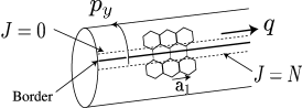
Figure 4: Geometry of graphene with the zigzag border. When $c=1$, the system becomes a graphene with zigzag edges since the hopping integral across the border is $-(1-c)\gamma_{0}$.

On the other hand, the localized states have several notable characteristics. First, localized state appears for $2\pi/3<q\leq\pi$ as we change $c$ from 0 to 1, i.e., there is an asymmetry about the K point in the momentum axis. Second, the two localized states gradually depart from the valence and conduction bands respectively as $c$ is increased (Fig. 2(d)). Third, those localized states merge when $c=1$ to become the flat bands with zero energy (Fig. 2(e)). In the following, we will analyze these features by analytically calculating the energy eigenvalue and localization length of localized state.

An energy eigenstate can be represented as

$$\psi_{E}(I,J)=N^{\prime}\exp(iqI)\begin{pmatrix}\phi_{\rm A}(J)\cr\phi_{\rm B}(J)\end{pmatrix}.$$ (39)

The energy eigenequation ${\cal H}(c)\psi_{E}=E\psi_{E}$ is written as

$$\begin{split}&\epsilon\phi_{\rm A}(J)=-\phi_{\rm B}(J+1)-Q\phi_{\rm B}(J),\\ &\epsilon\phi_{\rm B}(J+1)=-\phi_{\rm A}(J)-Q\phi_{\rm A}(J+1),\end{split}$$ (40)

where $Q\equiv 2\cos(q/2)$ and $\epsilon$ ($\equiv E/\gamma_{0}$) is the energy eigenvalue normalized by the hopping integral. The eigenstate is expressed as

$$\begin{pmatrix}\phi_{\rm A}(J)\cr\phi_{\rm B}(J)\end{pmatrix}=S_{J}\begin{pmatrix}Q+\frac{S_{J+1}}{S_{J}}&\epsilon\cr-\epsilon&-\left(Q+\frac{S_{J-1}}{S_{J}}\right)\end{pmatrix}\begin{pmatrix}\phi_{\rm A}(0)\cr\phi_{\rm B}(0)\end{pmatrix},$$

$$\ \ \ \ (J=0,\ldots,N)$$ (41)

where $S_{J}\equiv\sin(J\phi)/\sin\phi$. Here $\phi$ is a wavenumber in the direction of $J$ and satisfies

$$\epsilon^{2}=Q^{2}+2Q\cos\phi+1.$$ (42)

The derivation of eq. (41) is as follows: first, it is clear from eq.(40) that eq.(41) holds for $J=0$ and $J=1$. Second, let us rewrite eq.(40) using eq.(42) as

$$\begin{pmatrix}\phi_{\rm A}(J+1)\cr\phi_{\rm B}(J+1)\end{pmatrix}=\begin{pmatrix}Q+2\cos\phi&\epsilon\cr-\epsilon&-Q\end{pmatrix}\begin{pmatrix}\phi_{\rm A}(J)\cr\phi_{\rm B}(J)\end{pmatrix}.$$ (43)

Equation (41) can then be proved by induction.

The wave function is given by three parameters $c$, $q$ and $\phi$. The parameter $\phi$ is determined by the boundary condition: the energy eigenequation at border sites, $J=0$ (B sites) and $J=N$ (A sites),

$$\begin{split}&\epsilon\phi_{\rm B}(0)=-(1-c)\phi_{\rm A}(N)-Q\phi_{\rm A}(0),\\ &\epsilon\phi_{\rm A}(N)=-(1-c)\phi_{\rm B}(0)-Q\phi_{\rm B}(N).\end{split}$$ (44)

Equation (44) can be rewritten as

$$\begin{pmatrix}\phi_{\rm A}(N)\cr\phi_{\rm B}(N)\end{pmatrix}=\frac{1}{1-c}\begin{pmatrix}-Q&-\epsilon\cr\epsilon&\frac{\epsilon^{2}-(1-c)^{2}}{Q}\end{pmatrix}\begin{pmatrix}\phi_{\rm A}(0)\cr\phi_{\rm B}(0)\end{pmatrix}.$$ (45)

From eqs.(41) and (45), we obtain two equations relating $(\phi_{\rm A}(0),\phi_{\rm B}(0))$ to $(\phi_{\rm A}(N),\phi_{\rm B}(N))$. Then, by eliminating $\phi_{\rm A}(N)$ and $\phi_{\rm B}(N)$ in these equations, we obtain the following constraint equation for $\phi$,

$$\det\begin{pmatrix}(Q+\frac{S_{N+1}}{S_{N}})+\frac{Q}{A_{N}}&\epsilon(1+\frac{1}{A_{N}})\cr-\epsilon(1+\frac{1}{A_{N}})&-(Q+\frac{S_{N-1}}{S_{N}})-\frac{\Delta}{A_{N}}\end{pmatrix}=0,$$ (46)

where

$$A_{N}\equiv(1-c)S_{N},\ \ \Delta\equiv\frac{\epsilon^{2}-(1-c)^{2}}{Q}.$$ (47)

Equation (46) has $2N$ solutions of $\phi$ for given $N$. From the numerical calculation, we find that for $|Q|>1$, namely, for $0<q<2\pi/3$ or $4\pi/3<q<2\pi$, the equation has $2N$ real value solutions of $\phi$, and for $|Q|<1$ ($2\pi/3<q<4\pi/3$), it has $2(N-1)$ real value solutions (extended states) and 2 complex value solutions (localized states). As for localized state, $\phi$ can be parameterized as $\phi=i\ell/\xi$ or $\phi=\pi+i\ell/\xi$ depending on $-1<Q<0$ and $0<Q<1$, respectively. Here, $\xi$ is the localization length and thus when $\xi\to\infty$ the state becomes an extended state. From eq.(42), we have $\epsilon^{2}=(Q\pm 1)^{2}$ for $\phi=0$ and $\pi$. Thus, one can understand that there are two points in $(q,\phi)$ plane satisfying $\epsilon=0$, where a localized state turns into an extended state. [20] One point is located at $(2\pi/3,\pi)$ ($Q=1$) which is the K point and the other is located at $(4\pi/3,0)$ ($Q=-1$) which is the K^′ point.

When $N\gg 1$, by solving eq.(46) for localized state, we acquire

$$\frac{\ell}{\xi}=\ln\left(\frac{c(2-c)+\sqrt{c^{2}(2-c)^{2}+4Q^{2}(1-c)^{2}}}{2|Q|}\right)+\cdots,$$ (48)

where $\cdots$ denotes correction of ${\cal O}(e^{-N\ell/\xi})$ and therefore it is negligible when $N\gg\xi/\ell$. To obtain eq.(48), we neglected $A_{N}^{-2}$ in eq.(46) since $A_{N}$ is large as ${\cal O}(e^{N\ell/\xi})$. In this approximation, we get $Q(Q+e^{-\ell/\xi})+\Delta(Q+e^{\ell/\xi})=2\epsilon^{2}$ for $Q<0$. Using eqs.(42) and (47), we rewrite this condition as

$$(e^{\ell/\xi})^{2}-\frac{c(c-2)}{Q}e^{\ell/\xi}-(1-c)^{2}=0,$$ (49)

which gives eq.(48). The energy eigenvalue is obtained by inserting eq.(48) into eq.(42). It is to be noted that not only $c=0$ but also $c=2$ give no localized state since eq.(49) gives $\ell/\xi=0$ in these cases. For $c=2$, the hopping integral across the border is $+\gamma_{0}$, while other bonds are $-\gamma_{0}$. By a gauge transformation, this difference in sign of the hopping integral on the border can be absorbed into an AB phase $\pi$ around the nanotube (to the $y$-direction in Fig. 4). Thus the system is equivalent to a SWNT without border, with a $\pi$ flux (a half of the flux quantum) parallel to the NT axis. Because it has no border, it has no edge state.

Next, to understand $E$ and $\xi$ for localized state near the K point, we define the wave vector $k_{x}$ measured from K point as $q=2\pi/3+|\mathbf{a}_{1}|k_{x}$. Because $Q=2\cos(q/2)$, we have $Q=1-\ell k_{x}+(\ell k_{x})^{2}/6+{\cal O}((\ell k_{x})^{3})$. Then, from eq.(42) with $\phi=\pi+i\ell/\xi$, we obtain

$$\left(\frac{E}{v_{F}}\right)^{2}=p_{x}^{2}-\left(\frac{\hbar}{\xi}\right)^{2}+\cdots,$$ (50)

where $\cdots$ indicates higher order corrections such as $\ell p_{x}^{3}/\hbar$. The first two dominant terms in the right-hand side reproduce eq.(17). By expanding eq.(48) in terms of $p_{x}(=\hbar k_{x})$, we obtain eq.(18).

Finally, we check whether $E$ and $\xi$ of the continuous model reproduce the results of the TB model for localized states satisfying $k_{x}\ell\approx 1$. First, using eqs.(42) and (48), we plot $E$ and $\xi$ for $q=13\pi/18$, $7\pi/9$ and $8\pi/9$ as solid curves in Figs. 5(a) and 5(b), respectively. In Fig. 5(a), $E$ decreases slowly at small $c$. However, every curve decreases almost linearly as a function of $c$ for large $c$ and converges to zero. In Fig. 5(b) we see that $\xi$ decreases quickly with increasing $c$ and converge at $\xi/\ell=-1/\ln|Q|$ (eq.(48) with $c=1$). The convergence agrees with the previously published literatures. [2, 20] The dashed lines in Figs. 5(a) and 5(b) are $E$ and $\xi$ derived from the continuous model. The wave vectors $q=13\pi/18$, $7\pi/9$ and $8\pi/9$, which we used in the plot for the TB model, correspond to $|\mathbf{a}_{1}|k_{x}=\pi/18$, $\pi/9$ and $2\pi/9$, in the continuous model. Using eqs.(14) and (19), we plot $E/\gamma_{0}$ ($=\epsilon$) as dashed curves in Fig. 5(a). One can see that the solid and dashed curves are almost identical for $q=13\pi/18$. However, their difference is visible for $q=7\pi/9$ and not negligibly small for $q=8\pi/9$. Using eqs.(15) and (19), we plot $\xi/\ell$ as the dashed curves in Fig. 5(b). The continuous and the TB models agree with each other with $c$ near zero. For general $c$ and $q$, while the trend of $\xi$ agrees for the two models, their difference becomes large as the state is located apart from the K point. The discrepancy between the TB and continuous models comes from the assumption of the linear $k$ energy dispersion relation of the Weyl equation. The difference increases as the state is located apart from the Fermi point, which represents the deviation of the energy band from the linear energy dispersion. The energy dispersion relation may be improved to reproduce the TB model by adding some higher order terms to the Weyl equation.

Figure 5: (a) Energy eigenvalue $E/\gamma_{0}$ and (b) localization length $\xi/\ell$ as a function of $c$. The solid and dashed curves represent the TB model and the continuous model, respectively. Three wave vectors $q=13\pi/18$, $7\pi/9$ and $8\pi/9$ are chosen as examples. When $c=1$, each curve in (a) converges to zero, which agrees with the flat band of edge states, and each solid curve in (b) reproduces previous results of the localization length. [2, 20]

References

- [1] R. Saito, G. Dresselhaus and M.S. Dresselhaus: Physical Properties of Carbon Nanotubes, (Imperial College Press, London, 1998).
- [2] M. Fujita, K. Wakabayashi, K. Nakada and K. Kusakabe: J. Phys. Soc. Jpn. 65 (1996) 1920.
- [3] K. Nakada, M. Fujita, G. Dresselhaus and M.S. Dresselhaus: Phys. Rev. B 54 (1996) 17954.
- [4] Y. Niimi, T. Matsui, H. Kambara, K. Tagami, M. Tsukada and H. Fukuyama: Appl. Surf. Sci. 241 (2005) 43; Y. Niimi, T. Matsui, H. Kambara, K. Tagami, M. Tsukada and H. Fukuyama: arXiv:cond-mat/0601141.
- [5] Y. Kobayashi, K. Fukui, T. Enoki, K. Kusakabe and Y. Kaburagi: Phys. Rev. B 71 (2005) 193406; Y. Kobayashi, K. Fukui, T. Enoki and K. Kusakabe: arXiv:cond-mat/0602378.
- [6] J.C. Slonczewski and P.R. Weiss: Phys. Rev. 109 (1958) 272.
- [7] H. Ajiki and T. Ando: J. Phys. Soc. Jpn. 62 (1993) 2470.
- [8] S. Zaric, G. N. Ostojic, J. Kono, J. Shaver, V. C. Moore, M. S. Strano, R. H. Hauge, R. E. Smalley and X. Wei: Science 304 (2004) 1129.
- [9] C. L. Kane and E. J. Mele: Phys. Rev. Lett. 78 (1997) 1932.
- [10] M. Ouyang, J. Huang, C. L. Cheung and C. M. Lieber: Science 292 (2001) 27.
- [11] K. Sasaki, Y. Kawazoe and R. Saito: Prog. Theor. Phys. 113 (2005) 463.
- [12] J. Lee, H. Kim, S.-J. Kahng, G. Kim, Y.-W. Son, J. Ihm, H. Kato, Z. W. Wang, T. Okazaki, H. Shinohara and Y. Kuk: Nature 415 (2002) 1005.
- [13] T. Ando: J. Phys. Soc. Jpn. 74 (2005) 777.
- [14] D. J. Klein: Chem. Phys. Lett. 217 (1994) 261.
- [15] M. Fujita, M. Igami and K. Nakada: J. Phys. Soc. Jpn. 66 (1997) 1864.
- [16] K. Sasaki, S. Murakami and R. Saito: arXiv:cond-mat/0508442, Appl. Phys. Lett. (In press).
- [17] N.M.R. Peres, F. Guinea and A.H.C. Neto: arXiv:cond-mat/0506709 (unpublished); V.M. Pereira, F. Guinea, J.M.B. Lopes dos Santos, N.M.R. Peres and A.H.C. Neto: arXiv:cond-mat/0508530 (unpublished).
- [18] D. Porezag, Th. Frauenheim, Th. Köhler, G. Seifert and R. Kaschner: Phys. Rev. B 51 (1995) 12947.
- [19] T. Ando, T. Nakanishi and R. Saito: J. Phys. Soc. Jpn. 67 (1998) 2857.
- [20] K. Sasaki, S. Murakami, R. Saito and Y. Kawazoe: Phys. Rev. B 71 (2005) 195401.