Quantum optimal control theory and dynamic
coupling in the spin-boson model

Abstract

A Markovian master equation describing the evolution of open quantum systems in the presence of a time-dependent external field is derived within the Bloch-Redfield formalism. It leads to a system–bath interaction which depends on the control field. Optimal control theory is used to select control fields which allow accelerated or decelerated system relaxation, or suppression of relaxation (dissipation) altogether, depending on the dynamics we impose on the quantum system. The control–dissipation correlation and the non-perturbative treatment of the control field are essential for reaching this goal. The optimal control problem is formulated within Pontryagin’s minimum principle and the resulting optimal differential system is solved numerically. As an application, we study the dynamics of a spin-boson model in the strong coupling regime under the influence of an external control field. We show how trapping the system in unstable quantum states and transfer of population can be achieved by optimized control of the dissipative quantum system. We also used optimal control theory to find the driving field that generates the quantum Z-gate. In several cases studied, we find that the selected optimal field which reduces the purity loss significatively is a multi–component low–frequency field including higher harmonics, all of which lie below the phonon cutoff frequency. Finally, in the undriven case we present an analytic result for the Lamb shift at zero temperature.

I INTRODUCTION

In the theory of quantum information and computation, quantum coherence and entanglement are used as essential resources for efficient information processing Nielson . However, the interaction of the quantum system with its environment eventually leads to a complete loss of the information initially stored in its quantum state. This phenomena, known as decoherence, is regarded as a serious obstacle to a successful implementation of quantum information processing. The question of how it is possible to avoid the negative influence of this process is one of the most interesting issues in modern quantum mechanics. It not only concerns the area of quantum information and computation but many other fields of physics as well. The challenge is to preserve quantum coherence during a sufficiently long time needed for both storage and manipulation of the quantum states in systems which are unavoidably exposed to the influence of their surrounding environment.

Over the last few years, a number of interesting schemes have been proposed to eliminate the undesirable effects of decoherence in open quantum systems, including decoherence free subspaces Zanardi_1 ; Lidar , quantum error correction codes Nielson ; Preskill ; Knill , quantum feedback Wang and mechanisms based on the unitary “bang-bang” pulses and their generalization, quantum dynamical decoupling Viola_1 ; Viola_2 ; Zanardi_2 ; Vitali ; Uchiyama ; Byrd ; Protopopescu . The key ingredient of dynamical decoupling is the continuous disturbance of the system, which suppresses the system-environment interaction. It has been shown that, in the bang-bang control schemes, the decoherence of the system is effectively suppressed if the pulse rate is much higher than the decoherence rate due to the system-environment interaction. As already pointed out by Viola and Lloyd Viola_1 ; Viola_2 , the situation is similar to the so-called quantum Zeno effect Wayne which takes place in a system subject to frequent measurements projecting it onto its initial state: if the time interval between two projections is small enough the evolution of the system is nearly “frozen”. In a similar manner to the quantum Zeno effect, a fast rate control freezes decoherence. Analysis and comparison of the effects of these different physical procedures (bang-bang dynamic decoupling, coherence protection by the quantum Zeno effect and continuous coupling) have been investigated in Ref. Facchi . Advances in decoherence control using dynamical decoupling startegies is addressed in Ref. Viola_3 .

The staring point of the decoupling techniques is the observation that even though one does not have access to the large number of uncontrollable degrees of freedom of the environment, it is still possible to interfere with its dynamics by inducing motions into the system which are at least as fast as the environment dynamics Vitali . Moreover, if one can establish an additional coupling to the system by means of an external control, there can be quantum interference between the two interactions. The degree and nature of quantum interference – constructive or destructive – can be controlled by adjustment of the control field CCP .

In a simple–minded model of a dissipative quantum system, where the interference between the system–bath and system–control interaction is ignored or is irrelevant only limited control can be achieved Jirari . The situation changes dramatically when interference between the system–environment and system–control interaction can be used to control the effective system–environment coupling CCP ; Xu ; Kocharovskaya ; Schirr ; Morillon_1 ; Morillon_2 ; Dakhnovskii ; Grifoni ; Stigmunt_1 ; Stigmunt_2 ; Jirari_2 . This effect of coherent control of “dissipation” is demonstrated here for the example of the driven spin–boson model in which a quantum two-level system (qubit) is modelled by a spin, the environmental heat bath by quantum oscillators, and the spin subjected to an external control field is coupled to each bath oscillator independently. Decoherence control of this model is formulated using optimal control which is mathematically a problem of functional optimization under dynamical constraints Pontryagin ; ARTHURE ; Betts . Recently, we studied the same model with a control field restricted to a monochromatic wave plane Jirari_2 . The task was to find a set of three parameters namely the amplitude, the frequency and the phase using optimal control theory. Results were presented for control of the relative population of the spin system, i.e, the z-component of the Bloch vector. In the present paper, we show how this work can be extended to a control of all components of the Bloch vector simultaneously, as well as to general control field shapes.

The spin-boson model is a widely used model system. It can be mapped to a number of physical situations WEISS . In the theory of open quantum systems, the spin-boson model is actually one of the most popular models and has gained recent practical importance in the field of quantum computation Nielson . A special variant of it, in which the inter–level coupling is absent, is known as the independent–boson model Mahan . These models have been used to study the role of the electron–phonon interaction in point defects and quantum dots, interacting many–body systems, magnetic molecules, bath assisted cooling of spins and a two level Josephson-Junction  Kuhn ; Hohenester ; Zhang ; Luban ; Allahverdyan_1 ; Shon . Its basic properties have been reviewed in the literature Legget .

The remainder of the paper is organized as follows: in the next section we present a pedagogical derivation of Born-Markov master equations for dissipative N-level systems in the presence of time-dependent external control fields. The master equation is written as a set of Bloch-Redfield equations and a qualitative discussion of the influence of the control field on dissipation is given. This equation is the starting point for the derivation of the kinetic equation for the driven spin-boson model in the strong spin–boson coupling regime, as outlined in Sec. III. In Sec. IV, within the Pontryagin minimum principle we formulate the optimum control problem in terms of the Bloch vector. The general cost functional and its gradient in case of arbitrary control field are given. We also present the numerical approach in form of the gradient method. Our numerical results presented in Sec. V. Summary and conclusions are given in Sec. VI. Some mathematical details are relegated to appendixes.

II QUANTUM MASTER EQUATION FOR DRIVEN OPEN SYSTEMS

Consider a physical system $S$ embedded in a dissipative environment ($B$ also referred to as the heat bath) and interacting with a time-dependent classical external field, i.e., the control field. The Hilbert space of the total system ${\cal H}_{\rm tot}={\cal H}_{S}\otimes{\cal H}_{B}$ is expressed as the tensor product of the system Hilbert space ${\cal H}_{S}$ and the environment Hilbert space ${\cal H}_{B}$. The total Hamiltonian has the general form

$$H_{\rm tot}=H_{S}(t)+H_{B}+H_{\rm int}\,,$$ (1)

where $H_{S}(t)$ is the Hamiltonian of the system, $H_{B}$ of the bath and $H_{\rm int}$ of their interaction that is responsible for decoherence. The operators $H_{S}(t)$ and $H_{B}$ act on ${\cal H}_{S}$ and ${\cal H}_{B}$, respectively. The operator $H_{S}(t)$ contains a time-dependent external field to control the quantum evolution of the system.

II.1 Perturbation theory in the system-bath coupling

We shall be interested in the time evolution of the reduced density matrix of an open system, defined as

$$\rho_{S}(t)={\rm tr}_{B}\left\{\rho_{\rm tot}(t)\right\}\,.$$ (2)

where $\rho_{\rm tot}$ is the total density matrix for both the system and the bath. Here and in the following ${\rm tr}_{S}$ denotes the partial trace over the open system’s Hilbert space, while ${\rm tr}_{B}$ denotes the partial trace over the degrees of freedom of the environment $B$. A number of different methods are used to derive an equation of motion for the reduced density matrix Breuer . However, in any practical applications, two approximations are commonly invoked. The first is the initial factorization ansatz. Basically, one assumes that the interaction $H_{\rm int}$ is switched on at time $t=0$. Prior to this, the system $S$ and the environment $B$ are uncorrelated so that the initial density matrix of the total system factorizes as the product of the system and bath contributions, that is,

$$\rho_{\rm tot}(0)=\rho_{S}(0)\otimes\rho_{B}$$ (3)

with $\rho_{B}={\rm tr}_{S}\left\{\rho_{\rm tot}(0)\right\}$ and $\rho_{S}(0)={\rm tr}_{B}\left\{\rho_{\rm tot}(0)\right\}$. The second approximation is the weak system-bath interaction limit in which the second-order perturbation theory is applicable. In the following, we shall present a derivation of the master equation for $\rho_{S}$. $H_{\rm int}$ is assumed to be weak and will be treated perturbatively up to second order for its effects on $\rho_{S}$ under coherent external driving.

Let us start with the equation of motion for the total density matrix,

$$\dot{\rho}_{\rm tot}(t)=-\frac{i}{\hbar}\left[H_{\rm tot}(t),\rho_{\rm tot}(t)\right]\ .$$ (4)

The formal solution of the above equation can be obtained in the interaction picture Morillon_1 with respect to the Hamiltonian $H(t)=H_{S}(t)+H_{B}$,

$$\rho^{I}_{\rm tot}(t)=U^{\dagger}(t,0)\rho_{\rm tot}(t)U(t,0)\ ,$$ (5)

where the unitary operator reads

$$U(t,t^{\prime})={\cal T}\left\{\exp\left[-{i\over\hbar}\int_{t^{\prime}}^{t}\,d\tau\,H(\tau)\right]\right\}\ .$$ (6)

The time ordering ${\cal T}$ of the exponential in Eq. (6) is defined as the Taylor series with each term being time ordered. Using the fact that the operators $H_{S}(t)$ and $H_{B}$ commute

$$\left[H_{S}(t),H_{B}\right]=0$$ (7)

$U(t,t^{\prime})$ can be decomposed in the form

$$U(t,t^{\prime})=U_{S}(t,t^{\prime})\otimes U_{B}(t-t^{\prime})$$ (8)

with

$$U_{S}(t,t^{\prime})={\cal T}\left\{\exp\left[-{i\over\hbar}\int_{t^{\prime}}^{t}\,d\tau\,H_{S}(\tau)\right]\right\}$$ (9)

being the propagator of the coherent system dynamics satisfying the Schrödinger equation

$$i\hbar\frac{\partial}{\partial t}U_{S}(t,t^{\prime})=H_{S}(t)U_{S}(t,t^{\prime})$$ (10)

subject to the initial condition

$$U_{S}(t^{\prime},t^{\prime})={\cal I}\,,$$ (11)

and

$$U_{B}(t-t^{\prime})=\exp\left[-\frac{i}{\hbar}H_{B}(t-t^{\prime})\right]$$ (12)

is the propagator describing the free evolution of the environment. The equation of motion of $\rho^{I}_{\rm tot}$ is then

$$\dot{\rho}^{I}_{\rm tot}(t)=-\frac{i}{\hbar}\left[\ H_{I}(t),\rho^{I}_{\rm tot}(t)\right]$$ (13)

with $H_{I}(t)$ defined as

$$H_{I}(t)=U^{\dagger}(t,0)H_{\rm int}U(t,0)\,.$$ (14)

$H_{I}(t)$ is the interaction Hamiltonian written in the interaction picture. In integral form, Eq. (13) can be rewritten as

$$\rho^{I}_{\rm tot}(t)=\rho_{\rm tot}(0)-\frac{i}{\hbar}\int_{0}^{t}\,dt^{\prime}\left[\ H_{I}(t^{\prime}),\rho^{I}_{\rm tot}(t^{\prime})\right]$$ (15)

Inserting Eq. (15) into (13) and taking the trace over the bath we find the equation of motion for the reduced density matrix of the physical system

$$\dot{\rho}_{S}^{I}(t)=-\frac{1}{\hbar^{2}}\int_{0}^{t}\,dt^{\prime}{\rm tr}_{B}\left\{\left[H_{I}(t),\left[H_{I}(t^{\prime}),\rho^{I}_{\rm tot}(t^{\prime})\right]\right]\right\}\,.$$ (16)

We have assumed that (using Eq. (3))

$${\rm tr}_{B}\left\{\left[H_{I}(t),\rho_{\rm tot}(0)\right]\right\}={\rm tr}_{B}\left\{\left[H_{I}(t),\rho_{S}(0)\otimes\rho_{B}\right]\right\}=0$$ (17)

This assumption has to be justified when considering a specific case. Equation (16) still contains the density matrix of the total system $\rho^{I}_{\rm tot}(t)$ on its right-hand side. In order to eliminate $\rho^{I}_{\rm tot}(t)$ from the equation of motion, we assume that the interaction between the system and the environment is weak and perform the Born approximation Morillon_1 ; Breuer ; Blum

$$\rho^{I}_{\rm tot}(t^{\prime})=\rho^{I}_{S}(t^{\prime})\otimes\rho_{B}$$ (18)

In practice, one usually assumes a thermal equilibrium for the environment,

$$\rho_{B}=\frac{e^{-\beta H_{B}}}{{\rm tr}\,e^{-\beta H_{B}}}\,,$$ (19)

where $\beta=1/k_{B}T$ with $T$ the environment equilibrium temperature. Inserting the tensor product (18) in the exact equation of motion (16), we obtain a closed integro-differential equation for the reduced density matrix $\rho_{S}(t)$

$$\dot{\rho}_{S}^{I}(t)=-\frac{1}{\hbar^{2}}\int_{0}^{t}\,dt^{\prime}{\rm tr}_{B}\left\{\left[H_{I}(t),\left[H_{I}(t^{\prime}),\rho^{I}_{S}(t^{\prime})\otimes\rho_{B}\right]\right]\right\}\,.$$ (20)

In order to further simplify the above equation we perform the Markov approximation Morillon_1 ; Breuer ; Blum in which the integrant $\rho^{I}_{S}(t^{\prime})$ is replaced by $\rho^{I}_{S}(t)$

$$\dot{\rho}_{S}^{I}(t)=-\frac{1}{\hbar^{2}}\int_{0}^{t}\,dt^{\prime}{\rm tr}_{B}\left\{\left[H_{I}(t),\left[H_{I}(t^{\prime}),\rho^{I}_{S}(t)\otimes\rho_{B}\right]\right]\right\}\,.$$ (21)

The Markov approximation is therefore justified if the time scale $\tau_{R}$ over which the state of the system varies appreciably is large compared to the time scale $\tau_{B}$ over which the reservoir correlation functions decay ($\tau_{R}\gg\tau_{B}$). One now goes back to the Schrödinger picture using Eqs. (5), (14), the decomposition (8), and the cyclic invariance property of the trace

$${\dot{\rho}}_{S}(t)=-\frac{i}{\hbar}[H_{S}(t),\rho_{S}(t)]$$

$$~{}~{}-\frac{1}{\hbar^{2}}\int_{0}^{t}\,dt^{\prime}\mbox{tr}_{B}\left\{\left[H_{\rm int}(t-t^{\prime}),\left[\tilde{H}_{\rm int}(t,t^{\prime}),\rho_{S}(t)\otimes\rho_{B}\right]\right]\right\}\,.$$

Here

$$\tilde{H}_{\rm int}(t,t^{\prime})=U_{S}(t,t^{\prime})H_{\rm int}U_{S}^{\dagger}(t,t^{\prime})$$ (23)

is the interaction Hamiltonian in the anti-Heisenberg representation with respect to $H_{S}(t)$ and

$${H}_{\rm int}(t-t^{\prime})=U_{B}^{\dagger}(t-t^{\prime})H_{\rm int}U_{B}(t-t^{\prime})$$ (24)

the interaction Hamiltonian in the Heisenberg representation with respect to $H_{B}$. The time-evolution operators $U_{S}(t,t^{\prime})$ and $U_{B}(t-t^{\prime})$ are defined by Eqs. (9) and (12), respectively.

II.2 Bloch-Redfield equations

Let us suppose that ${\cal H}_{S}$ is an $N$-dimensional Hilbert space of orthonormal basis $|i\rangle,i=1\ldots N$. Writing the quantum master equation (II.1) in the representation $|i\rangle$ and expanding the double commutator, we obtain after some algebra Morillon_1 ; Blum

$${\dot{\rho}}_{S,ij}(t) = -\frac{i}{\hbar}\sum_{kl}\left(H_{S,ik}(t)\delta_{lj}-\delta_{ik}H_{S,lj}(t)\right)\,{\rho}_{S,kl}(t)$$ (25)

$$\qquad-\sum_{kl}{\cal R}_{ijkl}(t)\,{\rho}_{S,kl}(t)$$

where the first term represents the unitary part of the dynamics generated by the system Hamiltonian $H_{S}(t)$ and the second term accounts for the dissipative effects due to the coupling of the system to the environment. The Redfield relaxation tensor $R_{ijkl}(t)$ is given by

$${\cal R}_{ijkl}(t) = \delta_{lj}\sum_{r}\,\Gamma_{irrk}^{+}(t)+\delta_{ik}\sum_{r}\,\Gamma_{lrrj}^{-}(t)$$ (26)

$$\qquad-\Gamma_{ljik}^{+}(t)-\Gamma_{ljik}^{-}(t)$$

with the time-dependent rates $\Gamma_{ijkl}^{\pm}(t)$

$$\Gamma_{ljik}^{+}(t) = \frac{1}{\hbar^{2}}\int_{0}^{t}\,dt^{\prime}\,\mbox{tr}_{B}\left\{H_{{\rm int},lj}(t-t^{\prime}){\tilde{H}}_{{\rm int},{ik}}(t,t^{\prime})\rho_{B}\right\}\,,$$

$$\Gamma_{ljik}^{-}(t) = \frac{1}{\hbar^{2}}\int_{0}^{t}\,dt^{\prime}\,\mbox{tr}_{B}\left\{{\tilde{H}}_{{\rm int},{lj}}(t,t^{\prime})H_{{\rm int},{ik}}(t-t^{\prime})\rho_{B}\right\}\,.$$

Let us now write the Hamiltonian $H_{\rm int}$ in the Schrödinger picture in the following general form

$$H_{\rm int}=\sum_{\alpha}\,A_{\alpha}\otimes B_{\alpha}$$ (28)

where $A_{\alpha}$ and $B_{\alpha}$ are hermitian operators of the system and the environment, respectively. Inserting the expression (28) into Eqs. (27) and (27), using the fact that $A_{\alpha}$ and $B_{\alpha}$ commute leads to Morillon_1 ; Blum

$$\Gamma_{lj,ik}^{+}(t)=\frac{1}{\hbar^{2}}\int_{0}^{t}\,dt^{\prime}\sum_{\alpha,\beta}\left\langle B_{\alpha}(t-t^{\prime})B_{\beta}(0)\right\rangle_{B}A_{\alpha,{lj}}$$

$$\times\sum_{m,n}U_{S,{im}}(t,t^{\prime})A_{\beta,{mn}}U_{S,{kn}}^{\ast}(t,t^{\prime})\,,$$

(29a)

$$\Gamma_{lj,ik}^{-}(t)=\frac{1}{\hbar^{2}}\int_{0}^{t}\,dt^{\prime}\sum_{\alpha,\beta}\left\langle B_{\beta}(0)B_{\alpha}(t-t^{\prime})\right\rangle_{B}$$

$$\times\sum_{m,n}U_{S,{lm}}(t,t^{\prime})A_{\beta,{mn}}U_{S,{jn}}^{\ast}(t,t^{\prime})\,A_{\alpha,{ik}}\,,$$

where

$$\left\langle B_{\alpha}(\tau)B_{\beta}(0)\right\rangle_{B}={\rm tr}_{B}\left\{B_{\alpha}(\tau)B_{\beta}(0)\rho_{B}\right\}$$ (30)

is the environment correlation function with $\left\langle B_{\alpha}(0)B_{\beta}(\tau)\right\rangle_{B}=\left\langle B_{\alpha}(-\tau)B_{\beta}(0)\right\rangle_{B}$, since the environment is supposed to be in thermal equilibrium and its evolution is then homogeneous in time. Note that the condition (17) becomes

$$\left\langle B_{\alpha}(\tau)\right\rangle_{B}={\rm tr}_{B}\left\{B_{\alpha}(\tau)\rho_{B}\right\}=0,$$ (31)

which states that the reservoir averages of $B_{\alpha}(\tau)$ vanish.

The Born-Markov master equation (25) with the time-dependent decay rates defined in Eqs. (29) and (29) together with the Schrödinger equation (10) satisfied by the coherent time evolution operator $U_{S}(t,t^{\prime})$ provide all the necessary ingredients to describe the dynamics of a driven open quantum system. Note that the interaction of the system with the time-dependent control Hamiltonian $H_{S}(t)$ is treated non-perturbatively in the derivation of the above quantum master equation. The application of the present formulation to the driven spin–boson model in the weak coupling regime enables us to find an identical set of Bloch-Redfield equations obtained from projector-operator methods by Hartmann et al. Hartmann .

In the absence of the control field, $U_{S}(t,t^{\prime})\equiv U_{S}(t-t^{\prime})$ is the free time evolution operator of the physical system. In this particular case, the time integration in Eqs. (29) and (29) can be replaced by $\frac{1}{2}\int_{-\infty}^{+\infty}$ in the Markov approximation. After the extention of time integration to infinity, the decay rates $\Gamma_{ijkl}^{\pm}$ become time-independent and are then given in terms of the Fourier transform of the product of the environment correlation functions and the system dissipative operators (the interaction vertices), in agreement with the well-known results for undriven quantum open systems Blum .

II.3 Control field effects

The analysis of Eq. (25) shows that the presence of a time-dependent external field affects both the unitary evolution and the dissipative parts of the quantum master equation. The dissipative field influence can be interpreted as a direct consequence of quantum interference between the system-bath interaction and a coupling of the system to the external field. In order to study the dissipative field influence, let us examine the transition and the dephasing rates in the secular approximation Breuer ; Blum . In the zero field limit, the secular approximation assumes that the populations and the coherences are completely decoupled. It is valid if the typical time scale of the evolution of the system $\tau_{S}$, defined by a typical value for the inverse of the frequency associated with the system’s energy levels, is small compared to the relaxation time of the system, that is $\tau_{S}\ll\tau_{R}$. If we suppose that the secular approximation is still valid in the non-zero field case, the transition rates are defined as Kocharovskaya ; Schirr ; Blum

$$W_{ij}(t) = {\cal R}_{ii,jj}(t)$$ (32)

$$= \Gamma_{ji,ij}^{+}(t)+\Gamma_{ji,ij}^{-}(t)\,,$$

with $i\not=j$. Then, from the property $\left[\Gamma_{lj,ik}^{-}(t)\right]^{*}=\Gamma_{ki,jl}^{+}(t),$ it follows that the time dependent parameters $W_{ij}(t)$ are real, $W_{ij}^{*}(t)=W_{ij}(t)$. On the other hand, the dephasing rates are defined as Kocharovskaya ; Schirr ; Blum

$$\Gamma_{ij}(t)={\cal R}_{ij,ij}(t)=\sum_{r}\left[\Gamma_{ir,ri}^{+}(t)+\Gamma_{jr,rj}^{-}(t)\right]$$

$$\qquad\qquad-\Gamma_{jj,ii}^{+}(t)-\Gamma_{ii,jj}^{-}(t)\,.$$ (33)

The hermiticity condition of the density matrix implies $\Gamma_{ij}^{*}(t)=\Gamma_{ji}(t)$ which means that ${\Gamma}_{ij}(t)$ are complex numbers. In the zero field limit, the parameters $W_{ij}$ lead to a population relaxation into a thermal mixture of the system’s energy eigenvalues. Therefore, the diagonal elements of the density matrix decay to the value given by the Boltzmann factors. The real part of the parameters $\Gamma_{ij}(t)$ describes the dephasing, namely the decay of the off-diagonal elements of the density matrix towards zero. Their imaginary part leads to a renormalization of the system Hamiltonian which is induced by the vacuum fluctuation of the environment quantum operators (Lamb Shift). If a time-dependent external control field is applied, all these quantities become time-dependent (via the control field), and an external control of the dissipation is then possible. In particular, the correlation between the control field and the dissipation leads to the destruction of the detailed balance

$$\lim_{t\to\infty}{\frac{W_{ij}(t)}{W_{ji}(t)}}\not=\frac{\exp(-\beta E_{i})}{\exp(-\beta E_{j})}\,.$$ (34)

and allows for the control of the states populations. Here $E_{i}$ are the energy eigenvalues of the undriven physical system. Eq. (34) shows that the steady state can be far from equilibrium in the presence of a control field.

Taking the limit $\tau_{B}\to 0$ as a reasonable approximation, gives

$$\left\langle B_{\alpha}(\tau)B_{\beta}(0)\right\rangle_{B}\propto\delta_{\alpha\beta}\delta(\tau)$$ (35)

A random interaction with a $\delta$-correlation function is called white-noise, because the spectral distribution which is given by the Fourier transform of (35) is then independent of the frequency Risken . Substituting Eq. (35) into Eqs. (29) and (29), any field dependence disappears because $U_{S}(t,t)={\cal I}$. For classical problems the white-noise approximation holds when, in the high temperature limit, the environment resides within the classical regime and quantum effects may be ignored. In such a situation, the control-dissipation correlation disappears.

III DRIVEN spin–boson MODEL

III.1 The model

The driven spin–boson model consists of a two-level system interacting with a thermal bath in the presence of a time-dependent external control Grifoni ; Legget . The Hamiltonian for this model can be written as

$$H_{\rm tot}=H(t)+H_{\rm int}=H_{S}(t)+H_{B}+H_{\rm int}\,,$$ (36)

where the dynamics of the system $S$ is described by the Hamiltonian

$$H_{S}(t)=-\frac{\hbar}{2}\left(\Delta\sigma_{x}+\varepsilon_{0z}\sigma_{z}\right)-\frac{\hbar}{2}\varepsilon_{z}(t)\sigma_{z}\,.$$ (37)

Here $\sigma_{\alpha}$ with $\alpha=x,y,z$ are the Pauli spin matrices; $\hbar\Delta$ is the tunnelling splitting, $\hbar\varepsilon_{0z}$ is an energy bias and $\hbar\varepsilon_{z}(t)$ is its modulation by a time-dependent external control field. The Hamiltonian of the environment is assumed to be composed of harmonic oscillators with natural frequencies $\omega_{i}$ and masses $m_{i}$,

$$H_{B}=\sum_{i=1}^{N}\left(\frac{p_{i}^{2}}{2m_{i}}+\frac{m_{i}}{2}x_{i}^{2}\omega_{i}^{2}\right)\,,$$ (38)

where (${x}_{1},...,{x}_{N},{p}_{1},...,{p}_{N})$ are the coordinates and their conjugate momenta. The interaction between the system S and the environment B is assumed to be bilinear,

$$H_{\rm int}=\sum_{i=1}^{N}\,c_{i}\frac{q_{0}}{2}\sigma_{z}x_{i}\,,$$ (39)

where $c_{i}$ is the coupling constant between the spin coordinate and the $i$th environment oscillator with coordinate $q_{i}$ while $q_{0}$ measures the distance between the left and right potential wells. The coupling constants enter the spectral density function $J(\omega)$ of the environment defined by,

$$J(\omega)=\frac{\pi}{2}\sum_{i}\,{c_{i}\over m_{i}\,\omega_{i}}\,\delta(\omega-\omega_{i})\,.$$ (40)

III.2 Polaron transformation

The evaluation of the time-dependent Bloch-Redfield tensor ${\mathcal{R}}_{ijkl}(t)$ for the Hamiltonian (36), requires knowledge of the propagator of the coherent system dynamics $U_{S}(t,t^{\prime})$. Obtaining an analytical expression for $U_{S}(t,t^{\prime})$ is not trivial because the Hamiltonian of the physical system (37), is time-dependent and not diagonal. To get round this difficulty we perform the polaron transformation of the Hamiltonian (36). This transformation is defined by the unitary operatorLegget

$${\cal V}=e^{-\frac{i}{2}\sigma_{z}\Omega},$$ (41)

with

$$\Omega=\sum_{i}\Omega_{i},\quad\Omega_{i}=\left(q_{0}c_{i}/\hbar m_{i}\omega_{i}^{2}\right)p_{i}$$ (42)

Applied to the original Hamiltonian (36) leads to

$$H^{\prime}_{\rm tot}={\cal V}H_{\rm tot}{\cal V}^{-1}=H^{\prime}_{S}(t)+H^{\prime}_{B}+H^{\prime}_{\rm int}\,.$$ (43)

The expression

$$H^{\prime}_{S}(t)=-\frac{\hbar}{2}\left(\varepsilon_{0z}+\varepsilon_{z}(t)\right)\sigma_{z}\,,$$ (44)

is the internal system part of the transformed Hamiltonian

$$H^{\prime}_{B}=\frac{1}{2}\sum_{i}\left(\frac{p_{i}^{2}}{m_{i}}+m_{i}\omega_{i}^{2}x_{i}^{2}\right)\,,$$ (45)

defines the Hamiltonian of the bath, and

$$H^{\prime}_{\rm int}=-\frac{1}{2}\hbar\Delta\left(\sigma_{+}e^{-i\Omega}+\sigma_{-}e^{i\Omega}\right)\,,$$ (46)

gives the modified interaction. Here $\sigma_{\pm}=(\sigma_{x}\pm i\sigma_{y})/2$. After applying the polaron transformation the coherent propagator

$$U_{S}(t,t^{\prime})={\cal T}\left\{\exp\left[-{i\over\hbar}\int_{t^{\prime}}^{t}\,d\tau\,H^{\prime}_{S}(\tau)\right]\right\}$$ (47)

simplifies to

$$U_{S}(t,t^{\prime})=\cos\left[\left\{\varepsilon_{0z}(t-t^{\prime})+f(t,t^{\prime})\right\}/2\right]{\cal I}$$

$$\qquad+i\sin\left[\left\{\varepsilon_{0z}(t-t^{\prime})+f(t,t^{\prime})\right\}/2\right]\sigma_{z}$$ (48)

where ${\cal I}$ is the unit matrix of order $2\times 2$ and

$$f(t,t^{\prime})=\int_{t^{\prime}}^{t}\,d\tau\varepsilon_{z}(\tau)\,.$$ (49)

A constant phonon–induced energy shift in the system Hamiltonian has been omitted. As an application of the general formulation of the kinetic equation for driven open systems developed in Sec. (II), we will consider the Hamiltonian (43) and derive the explicit form of the corresponding master equation for small $\Delta$.

The physical situation described by this model can be envisioned as a weakly coupled (via $\Delta$) semiconductor double quantum dot containing a single electron. Each quantum dot provides one electronic level (spin is ignored). A metallic gate is located under each quantum dot. The relative bias between the two electrodes represents the control field. Alternatively, the Hamiltonian studied here can be interpreted as a spin 1/2–particle in a weak static B–field ($\varepsilon_{0}$, $\Delta$) which is directed slightly away from the z–direction in an external control field applied in z–direction.

For the transformed Hamiltonian, the interaction contribution is not the system–bath interaction, but rather accounts for a phonon–renormalized coupling between the two states ”up” and ”down”. Here, the dissipative operators of the system and those for the environment are $S_{1}=\hbar\Delta\sigma_{+}/2$, $S_{2}=S_{1}^{\dagger}=\hbar\Delta\sigma_{-}/2$ and $B_{1}=e^{-i\Omega}$, $B_{2}=B_{1}^{\dagger}=e^{i\Omega}$, respectively . For the new interaction Hamiltonian, Eq. (46), the rates $\Gamma_{ij,kl}^{\pm}(t)$ defined by Eqs. (29) and (29) may be written in terms of the equilibrium correlation functions with respect to the bosonic bath spectral density $J(\omega)$ in Eq. (40),

$$\langle e^{\pm i\Omega(t)}\,e^{\pm i\Omega(0)}\rangle_{B} = e^{-Q_{2}(t)}e^{iQ_{1}(t)}\,,$$ (50a)

$$\langle e^{\pm i\Omega(t)}\,e^{\mp i\Omega(0)}\rangle_{B} = e^{-Q_{2}(t)}e^{-iQ_{1}(t)}\,,$$ (50b)

$$\langle e^{\pm i\Omega(0)}\,e^{\pm i\Omega(t)}\rangle_{B} = e^{-Q_{2}(t)}e^{-iQ_{1}(t)}\,,$$ (50c)

$$\langle e^{\pm i\Omega(0)}\,e^{\mp i\Omega(t)}\rangle_{B} = e^{-Q_{2}(t)}e^{iQ_{1}(t)}\,,$$ (50d)

where the exponents are given by Mahan

$$Q_{1}(t) = \frac{q_{0}^{2}}{\pi\hbar}\int_{0}^{\infty}\,d\omega\frac{J(\omega)}{\omega^{2}}\sin(\omega t)\,,$$ (51a)

$$Q_{2}(t) = \frac{q_{0}^{2}}{\pi\hbar}\int_{0}^{\infty}\,d\omega\frac{J(\omega)}{\omega^{2}}(1-\cos(\omega t))\coth(\hbar\omega\beta/2)\,.$$

III.3 Ohmic spectrum of the bath

Within the present work, we consider the case of Ohmic spectrum

$$J(\omega)=\eta\omega e^{-\omega/\omega_{c}}=\left(2\pi\hbar\alpha/q_{0}^{2}\right)\omega e^{-\omega/\omega_{c}}\,.$$ (52)

Here $\eta$ is a phenomenological friction coefficient while $\alpha$ is the dimensionless coupling constant, and $\omega_{c}$ is an ultraviolet frequency cutoff. For the Ohmic bath (52), the functions $Q_{1}(\tau)$ in Eq. (51a) and $Q_{2}(\tau)$ in Eq. (51) can be determined explicitly Legget

$$Q_{1}(\tau) = 2\alpha\arctan(\omega_{c}\tau),$$ (53a)

$$Q_{2}(\tau) = 2\alpha\ln\left[\frac{{\bf\Gamma}^{2}\left(1+{1\over\hbar\omega_{c}\beta}\right)\sqrt{1+\omega_{c}^{2}\tau^{2}}}{{\bf\Gamma}\left(1+{1\over\hbar\omega_{c}\beta}-i{\tau\over\hbar\beta}\right){\bf\Gamma}\left(1+{1\over\hbar\omega_{c}\beta}+i{\tau\over\hbar\beta}\right)}\right]$$

where ${\bf\Gamma}$ is Euler’s Gamma function.

Let us determine the behaviour of the function $Q_{2}(\tau)$ at low temperature. Using the relation

$${\bf\Gamma}\left(1-i{\tau\over\hbar\beta}\right){\bf\Gamma}\left(1+i{\tau\over\hbar\beta}\right)=\frac{\pi\tau}{\beta\hbar}\frac{1}{\sinh\left(\pi\tau/\beta\hbar\right)}$$ (54)

one obtains from Eq. (53) for $\hbar\omega_{c}\beta\gg 1$ (low temperature)

$$Q_{2}(\tau)=\alpha\ln(1+\omega_{c}^{2}\tau^{2})+2\alpha\ln\left[\frac{\beta\hbar}{\pi\tau}\sinh\left(\frac{\pi\tau}{\beta\hbar}\right)\right]\,.$$ (55)

The first term is independent of temperature and describes how the fluctuations of the field vacuum affect the coherence of the open system. This contribution of $Q_{2}(\tau)$ to dissipation depends on the cutoff frequency $\omega_{c}$. The second term is the thermal contribution of $Q_{2}(\tau)$ to dissipation. Notice its dependence on the thermal correlation time $\tau_{B}=\beta\hbar/\pi$. On the other hand, the function $Q_{1}(\tau)$ is independent of temperature.

III.4 Master equation

For the description of the dynamics of a two-level system, it is convenient to map the state density matrix onto the Bloch vector ${\bf p}(t)=\left(p_{x}(t),p_{y}(t),p_{z}(t)\right)^{T}\in{\mathbb{R}^{3}}$ defined by

$${\bf p}(t)={\rm Tr}({\mbox{\boldmath$\sigma$}}\rho(t))=\left(\begin{array}[]{c}\rho_{01}(t)+\rho_{10}(t)\\ i(\rho_{01}(t)-\rho_{10}(t))\\ \rho_{00}(t)-\rho_{11}(t)\end{array}\right),$$ (56)

where ${\mbox{\boldmath$\sigma$}}=(\sigma_{x},\sigma_{y},\sigma_{z})$ is the vector composed of the three Pauli matrices. Within this notation, the states of a two-level system are parametrized by a 3-component vectors in the Bloch-sphere $B:=\left\{{\bf p}\in{\mathbb{R}^{3}};\,\|{\bf p}\|\leq 1\right\}$.

By combining the Redfield equation (25) with Eq. (56), we obtain for the Bloch vector the inhomogeneous linear equation of motion,

$$\dot{\bf p}(t)=\left({\mbox{\boldmath$\varepsilon$}}_{0}+{\mbox{\boldmath$\varepsilon$}}(t)\right)\times{\bf p}(t)+{\mbox{\boldmath$\xi$}}(t)\times\left({\bf p}(t)\times{\bf n}\right)$$

$$~{}~{}~{}~{}~{}~{}~{}~{}~{}~{}~{}~{}~{}~{}~{}-{\mbox{\boldmath$\gamma$}}(t)\,{\bf p}(t)+{\mbox{\boldmath$\gamma$}}_{0}(t)$$ (57)

with ${\mbox{\boldmath$\varepsilon$}}_{0}=(0,0,-\varepsilon_{0z})^{T}$, ${\mbox{\boldmath$\varepsilon$}}(t)=(0,0,-\varepsilon_{z}(t))^{T}$, ${\bf n}=(0,1,0)^{T}$,

$${\mbox{\boldmath$\xi$}}(t)=\left(\begin{array}[]{c}\xi(t)\\ 0\\ 0\end{array}\right)\,,\qquad{\mbox{\boldmath$\gamma$}}_{0}(t)=\left(\begin{array}[]{c}0\\ 0\\ \gamma_{0}(t)\end{array}\right)$$ (58)

and the relaxation matrix

$${\mbox{\boldmath$\gamma$}}(t)=\left(\begin{array}[]{c c c}0&0&0\\ 0&\gamma(t)&0\\ 0&0&\gamma(t)\end{array}\right).$$ (59)

where

$$\xi(t) = -{\rm Im}\left[{\mathcal{R}}_{12,12}(t)+{\mathcal{R}}_{12,21}(t)\right]$$

$$= -{\rm Im}\left[\Gamma^{+}_{12,21}(t)+\Gamma^{-}_{21,12}(t)-\Gamma^{+}_{12,12}(t)-\Gamma^{-}_{12,12}(t)\right]$$

$$\gamma(t) = {\rm Re}\left[{\mathcal{R}}_{11,11}(t)-{\mathcal{R}}_{11,22}(t)\right]$$ (60b)

$$= 2{\rm Re}\left[\Gamma^{+}_{12,21}(t)+\Gamma^{+}_{21,12}(t)\right]$$

and

$$\gamma_{0}(t) = -{\rm Re}\left[{\mathcal{R}}_{11,11}(t)+{\mathcal{R}}_{11,22}(t)\right]$$ (60c)

$$= -2{\rm Re}\left[\Gamma^{+}_{12,21}(t)-\Gamma^{+}_{21,12}(t)\right]$$

are linear combinations of the Redfield tensor elements. Eqs. (50a)-(50d), together with Eqs. (29) and (29) for the rates $\Gamma_{ij,kl}^{\pm}(t)$ , and the analytical expression of the coherent propagator (III.2) lead to

$$\xi(t)=\Delta^{2}\int_{0}^{t}\,d\tau\,e^{-Q_{2}(\tau)}\sin[\varepsilon_{0z}\tau+f(t,t-\tau)]\cos[Q_{1}(\tau)]$$

(61)

$$\gamma(t)=\Delta^{2}\int_{0}^{t}\,d\tau\,e^{-Q_{2}(\tau)}\cos[\varepsilon_{0z}\tau+f(t,t-\tau)]\cos[Q_{1}(\tau)]$$

(62)

$$\gamma_{0}(t)=\Delta^{2}\int_{0}^{t}\,d\tau\,e^{-Q_{2}(\tau)}\sin[\varepsilon_{0z}\tau+f(t,t-\tau)]\sin[Q_{1}(\tau)]$$

where the function $f(t,t^{\prime})$ is given in Eq. (49) while the functions $Q_{1}(t)$ and $Q_{2}(t)$ are defined in Eqs. (51a) and (51), respectively.

The control field dependence of the rates defined in Eqs. (III.4), (III.4) and the inhomogeneous term Eq. (III.4) enters via the function $f(t,t^{\prime})$ in Eq. (49). The quantity ${\mbox{\boldmath$\xi$}}(t)$ describes renormalization effects on the system Hamiltonian since it depends on the imaginary part of the Redfield tensor elements. It serves as an effective local–control field correction acting on the system. The relaxation and dephasing processes are determined by the rate ${\mbox{\boldmath$\gamma$}}(t)$. Note that the values for ${\mbox{\boldmath$\xi$}}(t)$, ${\mbox{\boldmath$\gamma$}}(t)$ and ${\mbox{\boldmath$\gamma$}}_{0}(t)$ at the current time $t$ depend on the control field ${\mbox{\boldmath$\varepsilon$}}(t^{\prime\prime})$ for $t^{\prime\prime}\in[0,t]$.

The explicit equations of motion for the components of the Bloch vector reads

$$\dot{p}_{x}(t) = \left(\varepsilon_{0z}+\varepsilon_{z}(t)\right)p_{y}(t)\,,$$ (64a)

$$\dot{p}_{y}(t) = -\left(\varepsilon_{0z}+\varepsilon_{z}(t)+\xi(t)\right)p_{x}(t)-\gamma(t)\,p_{y}(t)\,,$$

$$\dot{p}_{z}(t) = -\gamma(t)p_{z}(t)+\gamma_{0}(t)\,.$$ (64c)

We would like to emphasize here that the decoupling of the populations from the coherences follows from the polaron transformation and the perturbative expansion up to second order in the tunnelling coupling $\Delta$, and thus no secular approximation is required.

III.5 Undriven case

In order to illustrate the effects of the bath, namely the relaxation of the system and its energy renormalisation, we can analyse the master equation in the absence of the control field. The analytical expressions for the rates are worked out in the Appendixes. At zero temperature and for $\alpha>1/2$, the decay rate follows as

$$\left.\gamma(\varepsilon_{0z}>0)\right|_{T=0} = \frac{\pi\Delta^{2}}{2{\bf\Gamma}(2\alpha)}\left(\frac{1}{\omega_{c}}\right)^{2\alpha}\varepsilon^{2\alpha-1}_{0z}\,e^{-\left(\varepsilon_{0z}/\omega_{c}\right)}\,,$$

$$\left.\gamma(\varepsilon_{0z}<0)\right|_{T=0} = \frac{\pi\Delta^{2}}{2{\bf\Gamma}(2\alpha)}\left(\frac{1}{\omega_{c}}\right)^{2\alpha}\left(-\varepsilon_{0z}\right)^{2\alpha-1}\,e^{\left(\varepsilon_{0z}/\omega_{c}\right)}\,,$$

which agrees in leading order in $\varepsilon_{0z}/\omega_{c}$ with the result of Ref. Legget . Here ${\bf\Gamma}$ is the Euler’s Gamma function. A similar expression holds for the inhomogeneous term

$$\left.\gamma_{0}(\varepsilon_{0z}>0)\right|_{T=0} = \frac{\pi\Delta^{2}}{2{\bf\Gamma}(2\alpha)}\left(\frac{1}{\omega_{c}}\right)^{2\alpha}\varepsilon^{2\alpha-1}_{0z}\,e^{-\left(\varepsilon_{0z}/\omega_{c}\right)}\,,$$

$$\left.\gamma_{0}(\varepsilon_{0z}<0)\right|_{T=0} = -\frac{\pi\Delta^{2}}{2{\bf\Gamma}(2\alpha)}\left(\frac{1}{\omega_{c}}\right)^{2\alpha}\left(-\varepsilon_{0z}\right)^{2\alpha-1}\,e^{\left(\varepsilon_{0z}/\omega_{c}\right)}.$$

Next, we consider the effect of the bath on the energy splitting. By using the expression of $\xi(\varepsilon_{0z})$ from (116), we obtain

$$\left.\tilde{\varepsilon}_{0z}\right|_{T=0} = \left.{\varepsilon}_{0z}\times\left[1+\frac{\xi({\varepsilon}_{0z})}{{\varepsilon}_{0z}}\right]\right|_{T=0}$$

$$= \varepsilon_{0z}\times\left[1-\frac{\Delta^{2}}{\omega_{c}^{2}}\,\frac{\sinh\left(\varepsilon_{0z}/\omega_{c}\right)}{\left(\varepsilon_{0z}/\omega_{c}\right)}\,\frac{{\bf\Gamma}(2\alpha-2)}{{\bf\Gamma}(2\alpha)}\right]\,.$$

The last equation which is valid when $\frac{\varepsilon_{0z}}{\omega_{c}}\ll 1$ and $\alpha>1$ shows that $\xi({\varepsilon}_{0z})/{\varepsilon}_{0z}$ is negative and constitute one of the principal result of this work. The effect of $\xi({\varepsilon}_{0z})$ is the analogue of the Lamb shift, i.e. the renormalization of the level splitting in atoms due to the coupling to the electromagnetic radiations.

In thermal equilibrium, the system density matrix can be represented in the localised eigenstates $|R\rangle$ and $|L\rangle$ of the position operator $\sigma_{z}=\left(|R\rangle\langle R|-|L\rangle\langle L|\right)$ as

$$\rho=\frac{e^{\beta\hbar\varepsilon_{0z}\sigma_{z}/2}}{2\cosh\left(\beta\hbar\varepsilon_{0z}/2\right)}\,.$$ (68)

The equilibrium values of the Bloch-vector can be calculated from the density matrix, ${\bf p}_{\rm st}={\rm Tr}({\mbox{\boldmath$\sigma$}}\rho)$, yielding

$${\bf p}_{\rm st}=\left({p_{x}}_{\rm st},{p_{y}}_{\rm st},{p_{z}}_{\rm st}\right)^{T}=\left(\begin{array}[]{c}0\\ 0\\ \tanh(\hbar\beta\varepsilon_{0z}/2)\\ \end{array}\right)\,.$$ (69)

Equation (69) corresponds to the stationary solution of the master equation (III.4). From the rate equation (64c), it follows that the decay rate $\gamma({\varepsilon}_{0z})$ and the inhomogeneous term $\gamma_{0}({\varepsilon}_{0z})$ satisfies the detailed balance condition

$$\frac{\gamma_{0}(\varepsilon_{0z})}{\gamma(\varepsilon_{0z})}=\tanh(\hbar\beta\varepsilon_{0z}/2)\,,$$ (70)

which states that the process of absorption of phonons and its inverse, the process of emission of phonons, occur with equal probability in thermal equilibrium and arises from the following quantum property of the thermal equilibrium correlation function $\langle e^{i\Omega(-t)}\,e^{i\Omega(0)}\rangle_{B}=\langle e^{i\Omega(t-i\hbar\beta)}\,e^{i\Omega(0)}\rangle_{B}$.

III.6 Limits of validity of the polaron transformation

In the undriven case, the model with Hamiltonian (36) cannot be solved analytically, in general, and there are no reliable approximate methods which apply for a fixed (maybe weak) coupling to the bath and for all temperatures including the very low ones. For symmetric tunnelling $(\varepsilon_{0z}=0)$, application of perturbative theory in the Ohmic bath coupling leads to a non-analytical temperature dependence for the renormalized tunnelling $\Delta_{r}\propto T^{\alpha}$. At higher temperature there is a crossover from damped oscillations to over-damped motion, WEISS ; Legget ; Grabert with a relaxation rate that, in the weak coupling regime ($\alpha\ll 1$), decreases with increasing temperature, $\gamma\propto T^{2\alpha-1}$. The singular behaviour of the weak coupling series shows that perturbative theories break down at low temperature. On the other hand, the method of polaron transformation with the resulting Hamiltonian (43) is basically a perturbation theory in the tunnelling parameter $\Delta$ and is suitable for the strong coupling regime as we have shown in the last section. In fact, the combination of the polaron transformation with the second Born approximation is equivalent to a double path integral non-interacting blip approximation (NIBA) Pottier .

Recently, Vorrath et al. Vorrath used the combination of the polaron transformation with the Markov-Born approximation to derive a master equation for the generalisation of the undriven spin-boson model to spins greater than one-half in the strong coupling regime. They showed that this method is good enough if the parameters of the model, namely the temperature and the coupling, are limited to the case where the NIBA is valid. In the case of the driven spin boson model, the limits of the NIBA are discussed in Ref. Grifoni .

IV QUANTUM OPTIMAL CONTROL PROBLEM

Let the time $t$ be in the interval $[0,t_{F}]$ for fixed $t_{F}$. The evolution of the state variable ${\bf p}(t)$ governed by the master equation (III.4) depends not only on the initial state ${\bf p}(0)={\bf p}_{I}$ but also on the time-dependent control variable ${\mbox{\boldmath$\varepsilon$}}(t)$. The idea now is to seek the optimal form of the the control field that allows for steering the Bloch vector from the given initial state ${\bf p}(0)={\bf p}_{I}$ to a desired final state at a specified time $t_{F}$. Typically, it is possible to define a cost functional incorporating the objective. Then, the goal of optimal control algorithms is to calculate the control field which can induce a specific dynamics by minimizing this cost functional constraint by the state equation  ARTHURE ; Betts , i.e, the master equation (III.4) subject to the initial condition ${\bf p}(0)={\bf p}_{I}$.

IV.1 Cost functional

For the problems of interest here, the cost functional may be written as

$$J=\Phi\left[{\bf p}(t_{F})\right]+\int_{0}^{t_{F}}{\mathcal{L}}\left({\bf p}(t),{\mbox{\boldmath$\varepsilon$}}(t)\right)\,dt\,.$$ (71)

The functionals $\Phi\left[{\bf p}(t_{F})\right]$ and ${\mathcal{L}}\left({\bf p}(t),{\mbox{\boldmath$\varepsilon$}}(t)\right)$ account for the specific objective at the fixed target time $t_{F}$ and at intermediate times $t\in[0,t_{F}]$, respectively. J in Eq. (71) is the sum of the so-called final time cost functional and running cost functional.

IV.2 Pontryagin’s minimum principle

Consider the quantum optimal control problem of minimizing the cost functional (71) subject to the dynamical constraint (III.4):

$$\begin{cases}{\mbox{min}}\left\{J=\Phi\left[{\bf p}(t_{F})\right]+\int_{0}^{t_{F}}{\mathcal{L}}\left({\bf p}(t),{\mbox{\boldmath$\varepsilon$}}(t)\right)\,dt\right\}\\ \dot{\bf p}(t)=\left({\mbox{\boldmath$\varepsilon$}}_{0}+{\mbox{\boldmath$\varepsilon$}}(t)\right)\times{\bf p}(t)+{\mbox{\boldmath$\xi$}}(t)\times\left({\bf p}(t)\times{\bf n}\right)\\ \qquad\qquad-{\mbox{\boldmath$\gamma$}}(t){\bf p}(t)+{\mbox{\boldmath$\gamma$}}_{0}(t)\\ {\bf p}(0)={\bf p}_{I}\,,\quad t\in[0,t_{F}]\\ \end{cases}$$ (72)

An optimal solution of the problem (72) is characterized by first order optimality conditions in the form of the Pontryagin’s minimum principle Pontryagin ; ARTHURE ; Betts ; Jirari . These conditions are formulated with the help of the Hamilton function that has the following form in our problem:

$${\mathcal{H}}\left({\bf p}(t),{\mbox{\boldmath$\lambda$}}(t),{\mbox{\boldmath$\varepsilon$}}(t)\right)={\mathcal{L}}\left({\bf p}(t),{\mbox{\boldmath$\varepsilon$}}(t)\right)+$$ (73)

$${\mbox{\boldmath$\lambda$}}(t)\centerdot\left\{\left({\mbox{\boldmath$\varepsilon$}}_{0}+{\mbox{\boldmath$\varepsilon$}}(t)\right)\times{\bf p}(t)+{\mbox{\boldmath$\xi$}}(t)\times\left({\bf p}(t)\times{\bf n}\right)\right.$$

$$\left.~{}~{}~{}~{}-{\mbox{\boldmath$\gamma$}}(t){\bf p}(t)+{\mbox{\boldmath$\gamma$}}_{0}(t)\right\}\,,$$

where ${\bf\lambda(t)}$ is called the adjoint or the co–state variable, which is a Lagrange multiplier introduced to implement the constraint and thereby to render the variables ${\bf p}(t)$ and ${\mbox{\boldmath$\varepsilon$}}(t)$ independent. Following a variation in analogy to Hamilton’s variation principle of classical mechanics, the necessary first order optimality conditions result in a two-point boundary value problem:

$$\begin{cases}\dot{\bf p}(t)=\frac{\partial{\mathcal{H}}\left({\bf p}(t),{\mbox{\boldmath$\lambda$}}(t),{\mbox{\boldmath$\varepsilon$}}(t)\right)}{\partial{\mbox{\boldmath$\lambda$}}(t)},\quad t\in[0,t_{F}]\\ \\ \dot{\mbox{\boldmath$\lambda$}}(t)=-\frac{\partial{\mathcal{H}}\left({\bf p}(t),{\mbox{\boldmath$\lambda$}}(t),{\mbox{\boldmath$\varepsilon$}}(t)\right)}{\partial{\bf p}(t)},\qquad t\in[0,t_{F}]\\ \\ {\bf p}(0)={\bf p}_{I},\qquad{\mbox{\boldmath$\lambda$}}(t_{F})=\frac{\partial\Phi\left[{\bf p}(t_{F})\right]}{\partial{\bf p}(t_{F})}\\ \\ 0=\frac{\partial{\mathcal{H}}\left({\bf p}(t),{\mbox{\boldmath$\lambda$}}(t),{\mbox{\boldmath$\varepsilon$}}(t)\right)}{\partial{\mbox{\boldmath$\varepsilon$}}(t)},\quad t\in[0,t_{F}]\end{cases}$$ (74)

where the last condition is equivalent to the vanishing of the first variation of the cost functional,i.e, $\delta J=0$.

The minimum principle requires the solution of complicated nonlinear algebraic equations, namely, the optimality condition ${\partial{\mathcal{H}}}/{\partial{\mbox{\boldmath$\varepsilon$}}}=0$, which can only be solved in an iterative manner. The present optimal control problem (72) is not singular because ${\partial^{2}{\mathcal{H}}}/{\partial{\mbox{\boldmath$\varepsilon$}}^{2}}\not=0$, since ${\mbox{\boldmath$\xi$}}(t)$, ${\mbox{\boldmath$\gamma$}}(t)$ and ${\mbox{\boldmath$\gamma$}}_{0}(t)$ depend nonlinearly on ${\mbox{\boldmath$\varepsilon$}}(t)$ regardless of the choice of the running cost ${\mathcal{L}}$. Applying then the implicit function theorem one concludes that the optimality condition may have one solution, i.e, ${\mbox{\boldmath$\varepsilon$}}(t)=\left({\bf p}(t),{\mbox{\boldmath$\lambda$}}(t)\right)$ or more solutions which are only ”locally unique”. Here we apply the gradient method as an iterative scheme for solving (72).

Let us now explicitly compute the gradient of the cost functional with respect to the control field. For this we first write the equation of motion for the adjoint state $\lambda$. Eqs. (73) and (74 lead to

$$\dot{\mbox{\boldmath$\lambda$}}(t)=-\frac{\partial{\mathcal{L}}\left({\bf p}(t),{\mbox{\boldmath$\varepsilon$}}(t)\right)}{\partial{\bf p}(t)}+\left({\mbox{\boldmath$\varepsilon$}}_{0}+{\mbox{\boldmath$\varepsilon$}}(t)\right)\times{\mbox{\boldmath$\lambda$}}(t)$$

$$\qquad\qquad-\left({\mbox{\boldmath$\xi$}}(t)\times{\mbox{\boldmath$\lambda$}}(t)\right)\times{\bf n}+{\mbox{\boldmath$\gamma$}}^{T}(t){\mbox{\boldmath$\lambda$}}(t).$$ (75)

or in components form

$$\dot{\lambda}_{x}(t) = -\frac{\partial{\mathcal{L}}}{\partial{p_{x}}(t)}+\left(\varepsilon_{0z}+\varepsilon_{z}(t)+\xi(t)\right)\lambda_{y}(t)\,,$$ (76a)

$$\dot{\lambda}_{y}(t) = -\frac{\partial{\mathcal{L}}}{\partial{p_{y}}(t)}-\left(\varepsilon_{0z}+\varepsilon_{z}(t)\right)\lambda_{x}(t)+\gamma(t)\lambda_{y}(t)\,,$$

$$\dot{\lambda}_{z}(t) = -\frac{\partial{\mathcal{L}}}{\partial{p_{z}}(t)}+\gamma(t)\lambda_{z}(t)\,.$$ (76c)

Within the Pontryagin’s Minimum Principle, the variation of the cost functional (71) reads

$$\delta J = \int_{0}^{t_{F}}\frac{\delta J}{\delta{\mbox{\boldmath$\varepsilon$}}}\centerdot\delta{\mbox{\boldmath$\varepsilon$}}dt=\int_{0}^{t_{F}}\frac{\partial{\mathcal{H}}\left({\bf p}(t),{\mbox{\boldmath$\lambda$}}(t),{\mbox{\boldmath$\varepsilon$}}(t)\right)}{\partial{\mbox{\boldmath$\varepsilon$}}(t)}\centerdot\delta{\mbox{\boldmath$\varepsilon$}}(t)dt$$

$$= \int_{0}^{t_{F}}\left[\frac{\partial{\mathcal{L}}\left({\bf p}(t),{\mbox{\boldmath$\varepsilon$}}(t)\right)}{\partial{\mbox{\boldmath$\varepsilon$}}(t)}+\left({\mbox{\boldmath$\lambda$}}(t)\times{\bf p}(t)\right)\right]\centerdot\delta{\mbox{\boldmath$\varepsilon$}}(t)dt$$

$$+\int_{0}^{t_{F}}\frac{\partial}{\partial{\mbox{\boldmath$\varepsilon$}}(t)}\left[{\mbox{\boldmath$\lambda$}}(t)\centerdot\{{\mbox{\boldmath$\xi$}}(t)\times\left({\bf p}(t)\times{\bf n}\right)\}\right]\centerdot\delta{\mbox{\boldmath$\varepsilon$}}(t)dt$$

$$+\int_{0}^{t_{F}}\frac{\partial}{\partial{\mbox{\boldmath$\varepsilon$}}(t)}\left[{\mbox{\boldmath$\lambda$}}(t)\centerdot\left\{-{\mbox{\boldmath$\gamma$}}(t){\bf p}(t)+{\mbox{\boldmath$\gamma$}}_{0}(t)\right\}\right]\centerdot\delta{\mbox{\boldmath$\varepsilon$}}(t)dt\,.$$

The last equation enables us to compute the gradient of the cost functional with respect to the control field.

We may summarize the whole procedure for computing the gradient of the cost functional as follows: i) for a given control field ${\mbox{\boldmath$\varepsilon$}}(t)$, we first solve the state equation (III.4) forward in time, ii) the solution obtained for ${\bf p}$ is then used for the backward integration of the adjoint equation (IV.2), iii) with ${\bf p}$ and $\lambda$ obtained we compute the gradient.

Table 1: Best-fit parameters for a model defined by Eq. (90). $\Delta$ is the unit of the amplitudes $A_{i}$, $\Delta/2\pi$ of the frequencies $\nu_{i}$ and rd of the phases $\phi_{i}$. $\chi^{2}=36.43$.

Parameters	Fit	Error
$\nu$	0.354089322	2.431734350$\times 10^{-5}$
$A_{1}$	2.38068007	6.047635201$\times 10^{-3}$
$\phi_{1}$	-1.83291567	2.978756342$\times 10^{-3}$
$A_{2}$	2.79811789	6.033930931$\times 10^{-3}$
$\phi_{2}$	0.960902574	3.718809069$\times 10^{-3}$
$A_{3}$	-0.909244535	6.041502784$\times 10^{-3}$
$\phi_{3}$	0.65358378	8.091472983$\times 10^{-3}$
$A_{4}$	0.448104715	6.048448725$\times 10^{-3}$
$\phi_{4}$	-5.91914473	1.480647739$\times 10^{-2}$
$A_{5}$	0.144629845	6.054115543$\times 10^{-3}$
$\phi_{5}$	-9.41113677	4.260009231$\times 10^{-2}$
$A_{6}$	-0.0758863206	6.060940693$\times 10^{-3}$
$\phi_{6}$	2.94649922	8.029036597$\times 10^{-2}$
$A_{7}$	-0.0170884169	6.059845970$\times 10^{-3}$
$\phi_{7}$	-0.882323605	3.542289951$\times 10^{-1}$

IV.3 Discretization

By an appropriate discretization scheme, the above infinite dimensional constraint optimal control problem can be transformed into a finite dimensional optimization approximation ARTHURE ; Betts . For this purpose, we subdivide the time interval $[t_{1}=0,t_{F}]$ using

$$t_{j+1}=t_{j}+\Delta t,\quad j=1,\ldots,M-1\quad{\mbox{with}}\quad\Delta t=t_{F}/M$$ (78)

The values of the state, the adjoint and the control are evaluated at the mesh points $t_{j}$

$$\left({\bf p},{\mbox{\boldmath$\lambda$}},{\mbox{\boldmath$\varepsilon$}}\right)=\left({\bf p}_{1},\ldots,{\bf p}_{M},{\mbox{\boldmath$\lambda$}}_{1},\ldots,{\mbox{\boldmath$\lambda$}}_{M},{\mbox{\boldmath$\varepsilon$}}_{1},\ldots,{\mbox{\boldmath$\varepsilon$}}_{M}\right)^{T}\,\in{\mathbb{R}}^{9M}$$ (79)

where the following notation ${\bf p}(t_{j}):={\bf p}_{j}$, ${\mbox{\boldmath$\lambda$}}(t_{j}):={\mbox{\boldmath$\lambda$}}_{j}$ and ${\mbox{\boldmath$\varepsilon$}}(t_{j}):={\mbox{\boldmath$\varepsilon$}}_{j}$ is used.

Adopting the Euler scheme for solving the state equation (III.4) and the adjoint equation (IV.2) and by applying the Riemann-rule integration to the cost functional (71) and to its variation (IV.2), we obtain the main tool for solving the time-discrete formulation of the quantum optimal control problem defined in Eq. (72)

• state equation

  $${\bf p}_{j+1}={\bf p}_{j}+\Delta t\left[\left({\mbox{\boldmath$\varepsilon$}}_{0}+{\mbox{\boldmath$\varepsilon$}}_{j}\right)\times{\bf p}_{j}+{\mbox{\boldmath$\xi$}}_{j}\times\left({\bf p}_{j}\times{\bf n}\right)\right]$$

  $$\qquad\qquad-\Delta t\left[{\mbox{\boldmath$\gamma$}}_{j}{\bf p}_{j}+{{\mbox{\boldmath$\gamma$}}_{0}}_{j}\right]$$ (80)

  for $j=1,\ldots,M-1$ with ${\bf p}_{1}={\bf p}_{I}$

• adjoint equation

  $${\mbox{\boldmath$\lambda$}}_{j-1}={\mbox{\boldmath$\lambda$}}_{j}-\Delta t\left[-\frac{\partial{\mathcal{L}}\left({\bf p}_{j},{\mbox{\boldmath$\varepsilon$}}_{j}\right)}{\partial{\bf p}_{j}}+\left({\mbox{\boldmath$\varepsilon$}}_{0}+{\mbox{\boldmath$\varepsilon$}}_{j}\right)\times{\mbox{\boldmath$\lambda$}}_{j}\right]$$

  $$\qquad\qquad-\Delta t\left[\left({\mbox{\boldmath$\xi$}}_{j}\times{\mbox{\boldmath$\lambda$}}_{j}\right)\times{\bf n}+{\mbox{\boldmath$\gamma$}}^{T}_{j}{\mbox{\boldmath$\lambda$}}_{j}\right]$$ (81)

  for $j=M,\ldots,2$ with ${\mbox{\boldmath$\lambda$}}_{M}=\frac{\partial\Phi\left({\bf p}_{M}\right)}{\partial{\bf p}_{M}}$.

• cost functional

  $$J=\Phi\left({\bf p}_{M}\right)+\Delta t\sum_{j=1}^{M}\,{\mathcal{L}}\left({\bf p}_{j},{\mbox{\boldmath$\varepsilon$}}_{j}\right)$$ (82)

• variation of the cost functional

  $$\Delta J=\Delta t\sum_{j=1}^{M}\,\left[\frac{\partial{\mathcal{L}}\left({\bf p}_{j},{\mbox{\boldmath$\varepsilon$}}_{j}\right)}{\partial{\mbox{\boldmath$\varepsilon$}}_{j}}+\left({\mbox{\boldmath$\lambda$}}_{j}\times{\bf p}_{j}\right)\right]\centerdot\Delta{\mbox{\boldmath$\varepsilon$}}_{j}$$

  $$\qquad+\Delta t\sum_{j,k=1}^{M}\,\frac{\partial}{\partial{\mbox{\boldmath$\varepsilon$}}_{k}}\left[{\mbox{\boldmath$\lambda$}}_{j}\centerdot\left\{{\mbox{\boldmath$\xi$}}_{j}\times\left({\bf p}_{j}\times{\bf n}\right)\right\}\right]\centerdot\Delta{\mbox{\boldmath$\varepsilon$}}_{k}$$

  $$+\Delta t\sum_{j,k=1}^{M}\,\frac{\partial}{\partial{\mbox{\boldmath$\varepsilon$}}_{k}}\left[{\mbox{\boldmath$\lambda$}}_{j}\centerdot\left\{-{\mbox{\boldmath$\gamma$}}_{j}{\bf p}_{j}+{{\mbox{\boldmath$\gamma$}}_{0}}_{j}\right\}\right]\centerdot\Delta{\mbox{\boldmath$\varepsilon$}}_{k}$$

• gradient of the cost functional

  $$\frac{\partial J}{\partial{\mbox{\boldmath$\varepsilon$}}_{i}}=\Delta t\left[\frac{\partial{\mathcal{L}}\left({\bf p}_{i},{\mbox{\boldmath$\varepsilon$}}_{i}\right)}{\partial{\mbox{\boldmath$\varepsilon$}}_{i}}+{\mbox{\boldmath$\lambda$}}_{i}\times{\bf p}_{i}\right]$$

  $$+\Delta t\sum_{j=1}^{M}\,\frac{\partial}{\partial{\mbox{\boldmath$\varepsilon$}}_{i}}\left[{\mbox{\boldmath$\lambda$}}_{j}\centerdot\left\{{\mbox{\boldmath$\xi$}}_{j}\times\left({\bf p}_{j}\times{\bf n}\right)-{\mbox{\boldmath$\gamma$}}_{j}{\bf p}_{j}+{{\mbox{\boldmath$\gamma$}}_{0}}_{j}\right\}\right]$$

  for $i=1,\ldots,M$.

The projection of (• ‣ IV.3) on the z-axis of the Bloch sphere leads to

$$\frac{\partial J}{\partial\varepsilon_{zi}}=\Delta t\left[\frac{\partial{\mathcal{L}}\left(p_{xi},p_{yi},p_{zi},\varepsilon_{zi}\right)}{\partial\varepsilon_{zi}}+\left(\lambda_{xi}p_{yi}-\lambda_{yi}p_{xi}\right)\right]$$

$$\qquad\qquad-\Delta t\sum_{j=1}^{M}\,\lambda_{yj}\left[\frac{\partial\xi_{j}}{\partial\varepsilon_{zi}}p_{xj}+\frac{\partial\gamma_{j}}{\partial\varepsilon_{zi}}p_{yj}\right]$$

$$\qquad\qquad+\Delta t\sum_{j=1}^{M}\,\lambda_{zj}\left[-\frac{\partial\gamma_{j}}{\partial\varepsilon_{zi}}p_{zj}+\frac{\partial\gamma_{0j}}{\partial\varepsilon_{zi}}\right]$$ (85)

for $i=1,\ldots,M$

The matrices ${\partial\xi_{j}}/{\partial\varepsilon_{i}}$, ${\partial\gamma_{j}}/{\partial\varepsilon_{i}}$ and ${\partial\gamma_{0j}}/{\partial\varepsilon_{i}}$ of size $M\times M$ are not diagonal because in the time-continuous problem $\xi(t)$, $\gamma(t)$ and $\gamma_{0}(t)$ at the current time $t$ depend on the control field at $t^{\prime}\leq t$ via the function (49).

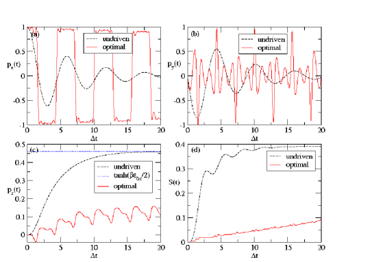
Figure 1: Implementation of the Z-gate with ${\bf p}_{I}=(1,0,0)^{T}$ and ${\bf p}_{d}=(-1,0,0)^{T}$. Depicted are the Bloch vector ${\bf p}=\left(p_{x},p_{y},p_{z}\right)^{T}$ and the linear entropy $S=\frac{1}{2}\left(1-||{\bf p}||^{2}\right)$ as a function of time for undriven case and for driven by the optimal control field obtained by the conjugate gradient method. (a), (b) and (c) show, respectively, the results for $p_{x}$ , $p_{y}$ and $p_{z}$ while (d) show the results for $S$. The parameters used are $\alpha=0.2$, $\varepsilon_{0z}=\Delta$, $\omega_{c}=20\Delta$ and $k_{B}T=\beta^{-1}=\hbar\Delta$. The final time is set as $t_{F}=20/\Delta$ and the chosen time step is $10^{-2}/\Delta$ corresponding to $M=2\times 10^{3}$ as the number of mesh points, i.e, the dimension of the optimal control problem.

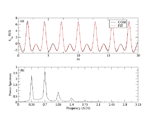
Figure 2: Implementation of the Z-gate with ${\bf p}_{I}=(1,0,0)^{T}$ and ${\bf p}_{d}=(-1,0,0)^{T}$. The upper panel (a) shows the optimal control field selected by the conjugate gradient method (CGM) vs. time while the lower panel (b) shows its power spectrum. A comparison with the model fit defined by Eq. (90) is also shown in the upper panel (a). Parameters as in Fig. 1.

IV.4 Numerical method

The set of equations needed to solve the optimal control problem (72) are the discrete-time versions of the cost functional $J(\varepsilon_{z1}\ldots,\varepsilon_{zM})$ defined in Eq. (82), the equation of motion for the state and the adjoint variables given by Eqs. (• ‣ IV.3) and (• ‣ IV.3), respectively, and the gradient of the cost functional ${\nabla}J(\varepsilon_{z1}\ldots,\varepsilon_{zM})$ in the form of Eq. (IV.3).

If we can compute the cost functional and its gradient at arbitrary points $\varepsilon_{z}=(\varepsilon_{z1}\ldots,\varepsilon_{zM})^{T}\in{\mathbb{R}}^{M}$, the general form of the gradient algorithm for minimization is as follows Frederic

1. Initialization: the initial guess ${\varepsilon_{z}^{1}}\in{\mathbb{R}}^{M}$ and the stopping tolerance tol $>0$ are given; set i=1.

2. Stopping test:

   • integrate the state equation forward in time to find ${\bf p}$.

   • integrate the adjoint equation backward in time to find $\lambda$

   • compute the gradient $\nabla J(\varepsilon_{z}^{1})$;

     if $\left|\nabla J(\varepsilon_{z}^{1})\right|\leq$ tol stop.

3. Computing the direction: compute the descent direction ${d^{i}}\in{\mathbb{R}}^{M}$ defined by $\nabla J(\varepsilon_{z}^{i})\centerdot{d^{i}}<0$.

4. Line-search: find an appropriate stepsize $\mu^{i}>0$ satisfying $J(\varepsilon_{z}^{i}+\mu^{i}\,d^{i})<J(\varepsilon_{z}^{i})$

5. Loop: set $\varepsilon_{z}^{i+1}=\varepsilon_{z}^{i}+\mu^{i}\,{d^{i}}$; increase i by 1 and go to 2.

In the work described here, the optimization of the cost functional is performed by using the subroutine FRPRMN of the Numerical Recipes package NRC which implements the conjugate gradient method as a variant of the above descent algorithm . We also used the subroutine DMNG of PORT library port implementing the quasi-Newton method. These two iterative methods of optimization are very popular. Both of them require the gradient but differ in the calculation of the descent direction.

The equations of motion for the state and the adjoint variables are forward and backward initial value problems, respectively. We solved them using the Euler scheme or a Runge-Kutta scheme which requires the values for the control field only at a grid point (see Sec. IV.3). Evaluation of the state and the adjoint variables involves an extensive computation of the time-dependent rates which are given by an integral over time of a rapidly oscillating functions (see Eqs. (III.4), (III.4), (III.4), (53a) and (53)). The numerical evaluation of the rate functions and their derivatives with respect to the control field involved in the computation of the gradient are performed using a Gauss quadrature suitable for an integration of rapidly oscillating functions.

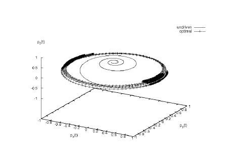
Figure 3: Implementation of the Z-gate with ${\bf p}_{I}=(1,0,0)^{T}$ and ${\bf p}_{d}=(-1,0,0)^{T}$. The 3-dimensional plot of the the Bloch vector ${\bf p}=\left(p_{x},p_{y},p_{z}\right)^{T}$ for undriven case and for driven by the optimal control field obtained by the conjugate gradient method is presented. Parameters as in Fig. 1.

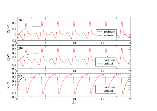
Figure 4: Implementation of the Z-gate with ${\bf p}_{I}=(1,0,0)^{T}$ and ${\bf p}_{d}=(-1,0,0)^{T}$. Depicted are the decay rate $\gamma$, the Lamb shift $\xi$ and the inhomogeneous term $\gamma_{0}$ as a function of time for undriven case and driven by the optimal control field selected by the conjugate gradient method. (a), (b) and (c) show, respectively, the results for $\gamma_{0}$, $\xi$ and $\gamma$. Parameters as in Fig. 1.

V NUMERICAL RESULTS

V.1 Z gate

As a first application of the quantum optimal control theory developed in Sec. IV, we consider the action of the Z gate

$$Z=\left(\begin{array}[]{c c}1&0\\ 0&-1\end{array}\right),$$ (86)

which leaves $|0\rangle$ unchanged, and flips $|1\rangle$ to $-|1\rangle$. Its application to the initial state $|\psi\rangle=\left(|0\rangle+|1\rangle\right)/\sqrt{2}$ leads to $|\psi\rangle^{\prime}=\left(|0\rangle-|1\rangle\right)/\sqrt{2}$. In term of the density matrix or the Bloch vector, we have for this particular state

$$\begin{CD}\rho=\frac{1}{2}\left(\begin{array}[]{c c}1&1\\ 1&1\end{array}\right)@>{Z}>{}>\rho^{\prime}=\frac{1}{2}\left(\begin{array}[]{c c}1&-1\\ -1&1\end{array}\right)\\ @V{}V{}V@V{}V{}V\\ {\bf p}=\left(\begin{array}[]{c}1\\ 0\\ 0\\ \end{array}\right)@>{Z}>{}>{\bf p}^{\prime}=\left(\begin{array}[]{c}-1\\ 0\\ 0\\ \end{array}\right)\end{CD}$$ (87)

The action of the dissipative Z-gate is phrased as an optimization problem. At time $t_{I}=0$ the two-level system (qubit) is prepared in the initial state ${\bf p}_{I}=(1,0,0)^{T}$. Our objective is to bring it into the desired state ${\bf p}_{d}=(-1,0,0)^{T}$ at time $t=t_{F}$. In this case, we need to minimize the deviation of the state of the system at final time ${\bf p}(t_{F})$ from the desired state ${\bf p}_{d}$. The cost functional chosen for this task is

$$J=\frac{1}{2}\|{\bf p}(t_{F})-{\bf p}_{d}\|^{2}~{}~{},$$ (88)

corresponding to the running cost functional ${\mathcal{L}}\left({\bf p}(t),{\mbox{\boldmath$\varepsilon$}}(t)\right)=0$ for all $t\in[0,t_{F}]$ and to the final cost functional $\Phi\left[{\bf p}(t_{F})\right]=\frac{1}{2}\|{\bf p}(t_{F})-{\bf p}_{d}\|^{2}$ in Eq. (71). The cost functional defined in Eq. (88) requires ${\mbox{\boldmath$\lambda$}}(t_{F})={\bf p}(t_{F})-{\bf p}_{d}$ as the initial condition in Eq. (IV.2) for the backward integration of the adjoint state variables $\lambda$.

Fig. 1 shows the components of the Bloch vector versus time and the evolution of the linear entropy defined by Breuer

$$S(t)=(1-\|{\bf p}(t)\|^{2})/2.$$ (89)

The dashed lines give the result for the case of zero control $\varepsilon(t)=0$. The solid lines give the results for the optimum field which was obtained by starting from a zero initial field and allowing 20 iterations. Fig. 2 shows the optimal field versus time, as well as its power spectrum. It can be seen that the selected field performs several abrupt switch operations between initial state ${\bf p}_{I}=(1,0,0)^{T}$ and target state ${\bf p}_{d}=(-1,0,0)^{T}$ to arrive at the target state at time $t_{F}$. In principle the Z–gate operation is completed at approximately time $t=2.5\Delta$. However, here we are interested in preventing the decrease of the Bloch vector over a prolonged period of time. The physical interpretation to the selected solution is the following: inspection of the kinetic equations for the Bloch vector Eqs.(64a), (64 and (64a) shows that a static field ${\varepsilon_{z}}_{\mbox{opt}}(t)=-\varepsilon_{0z}$ makes $(p_{x},0,0)^{T}$, for $-1\leq p_{x}\leq+1$ a stable (“decoherence–free”) subspace of the driven system. In this optimization run, the gradient selected a multiple switching version, whereby the system is, approximately, switched between the decoherence–free states ${\bf p}(t)=(1,0,0)^{T}$ and ${\bf p}(t)=(-1,0,0)^{T}$. Dissipation essentially is initiated during the first switching operation when there is a small build–up in $p_{y}$ and $p_{z}$ component, as can be seen by inspection of Fig 1(d) showing the linear entropy of the system. The latter increases almost linearly with time, however, at a greatly reduced rate when compared to the time–evolution of the undriven system. The situation is complicated because $p_{z}$ has a thermal equilibrium state at around $0.46$. As one sees in Fig. 1(c), the optimal field succeeds repeatedly in driving the $p_{z}(t)$ back towards zero. The evolution of the 3-d Bloch vector is shown in Fig. 3. While the control–free evolution rapidly spirals towards the thermal equilibrium state ${\bf p}_{\mbox{st}}=(0,0,\tanh(\hbar\beta\varepsilon_{0z}/2))^{T}$ the selected optimum control field is able to stabilize the Bloch vector and eventually drive it very near to the target state ${\bf p}_{d}=(-1,0,0)^{T}$.

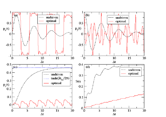
Figure 5: Implementation of the Z-gate with ${\bf p}_{I}=(0,1,0)^{T}$ and ${\bf p}_{d}=(0,-1,0)^{T}$. Depicted are the Bloch vector ${\bf p}=\left(p_{x},p_{y},p_{z}\right)^{T}$ and the linear entropy $S=\frac{1}{2}\left(1-||{\bf p}||^{2}\right)$ as a function of time for undriven case and for driven by the optimal control field obtained by the conjugate gradient method. (a), (b) and (c) show, respectively, the results for $p_{x}$ , $p_{y}$ and $p_{z}$ while (d) show the results for $S$. Parameters as in Fig. 1

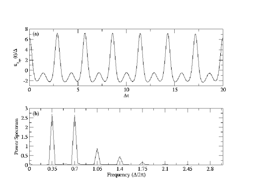
Figure 6: Implementation of the Z-gate with ${\bf p}_{I}=(0,1,0)^{T}$ and ${\bf p}_{d}=(0,-1,0)^{T}$. The upper panel (a) shows the optimal control field selected by the conjugate gradient method (CGM) vs. time while the lower panel (b) shows its power spectrum.

Fig 2(a) displays the time evolution of the selected optimal field. The repeated switching of the Bloch vector is achieved by a nearly periodic field. The essence of the Z–gate operation is more or less contained in one period. The electric field oscillates about the value $\varepsilon_{\mbox{o}pt}(0)\sim-\varepsilon_{0z}$ to trap the system in state ${\bf p}=(\pm 1,0,0)$. The switching is performed by a positive pulse which is optimized to rotate the Bloch vector into state ${\bf p}=(\mp 1,0,0)^{T}$. Then the field goes negative again to trap the system in this state. Performing more iterations will smoothen the oscillation about $\varepsilon_{\mbox{o}pt}(0)\sim-\varepsilon_{0z}$ and reduce the slope in the rise of the linear entropy. The analysis of Figs. 1 and 2 shows that the small oscillations of the control field about the value $-\varepsilon_{0z}$ between two switching operations (two positive pulses) are reflected in the time evolution of the Bloch vector.

The influence of the control–field on the dissipative part of the kinetic equations and the energy renormalization is displayed in Fig. 4 showing $\gamma_{0}$, $\gamma$, and $\xi$ versus time for the driven and undriven case. The periodic structure of the optimal control field manifests itself in both of them. The renormalization term $\xi$ and $\gamma_{0}$ resemble, essentially, a shifted and rescaled version of the control field itself. In this fashion they optimize support for the action of the electric field, in particular, when the latter rises to perform a switching operation. The minima of the relaxation rate $\gamma$, on the other hand, occur when the control field becomes large. In this way, dissipation during the switching process is minimized.

Fig 2(b) displays the power spectrum of the selected optimal control field showing seven pronounced peaks at near equidistant frequencies. So, the selected optimal control field can be approximated by

$${\varepsilon_{z}}^{{\small\mbox{FIT}}}(t)=\sum_{n=1}^{7}\,A_{n}\sin(2\pi n\nu t+\phi_{n})$$ (90)

depending on $15$ adjustable parameters which we determine using a nonlinear least square method consisting of minimizing the $\chi^{2}$ merit function defined by

$$\chi^{2}=\frac{1}{2}\sum_{i=1}^{M}\left[{\varepsilon_{z}}^{{\small\mbox{CGM}}}(t_{i})-{\varepsilon_{z}}^{{\small\mbox{FIT}}}(t_{i})\right]^{2}$$ (91)

where $M=2000$ is the number of mesh points and ${\varepsilon_{z}}^{{\small\mbox{CGM}}}(t_{i})$ is the optimal control field shown in Fig 2(a), solid line. The results are presented in Tab. 1. The value of the fit parameter $\nu=\left(0.35409\pm 2.43173\times 10^{-5}\right)\frac{\Delta}{2\pi}$ corresponding to the first peak of the power spectrum in Fig 2(b). The remaining higher frequency peaks are located at about $n\nu,n=2\ldots 7$. Tab. 1 shows that the amplitudes $A_{n}$ satisfy $|A_{2}|>|A_{1}|>|A_{3}|>\ldots>|A_{7}|$ while the phases $\phi_{n}$ alternate in their sign. In Fig. 2(a) we compare the optimal control field selected by the conjugate gradient method with the model defined by Eq. (90).

We also studied flipping from state ${\bf p}_{I}=(0,1,0)^{T}$ to ${\bf p}_{d}=(0,-1,0)^{T}$. The results are presented in Figs. 5-8. The same picture emerges. The optimized field immediately drives the system into state ${\bf p}=(1,0,0)^{T}$, performs switching between the decoherence-free states ${\bf p}=(1,0,0)^{T}$ and ${\bf p}=(-1,0,0)^{T}$, and finally transfers it into the target state ${\bf p}=(0,-1,0)^{T}$. Actually, Fig 6 displays the time evolution of the selected optimal field and its power spectrum. It is seen in Fig. 6(a) that the optimal control field starts out positive value to transfer the system from ${\bf p}_{I}=(0,1,0)^{T}$ to ${\bf p}=(1,0,0)^{T}$ and goes negative value (approximately $-\varepsilon_{0z}$) to trap the system in this state. The switching is performed by a positive pulse which is optimized to rotate the Bloch vector into state ${\bf p}=(-1,0,0)^{T}$. Then the field goes negative again to trap the system in this state. After, performing several abrupt switch operations between the free-decohrence states ${\bf p}=(1,0,0)^{T}$, ${\bf p}=(-1,0,0)^{T}$, the control field value at the final time $t_{F}$ is positive in order to transfer the system into the target state ${\bf p}=(0,-1,0)^{T}$. Contrary to the first example, the configurations ${\bf p}=(0,p_{y},0)^{T}$ for $-1\leq p_{y}\leq+1$ are not stable under external driving by a negative static control field ${\varepsilon_{z}}(t)=-\varepsilon_{0z}$. Thereby, the control optimum field value is positive at the beginning and also at end of the time evolution interval $[0,t_{F}]$ allowing the transfer of the system from ${\bf p}=(0,1,0)^{T}$ to ${\bf p}=(1,0,0)^{T}$ at the initial time and from ${\bf p}=(1,0,0)^{T}$ to the target state ${\bf p}=(0,-1,0)^{T}$ at a final time as it is illustrated in Figs. 5 and 6(a). Fig 6(b) shows that the power spectrum displays seven pronounced peaks at equidistant frequencies similar to the first example. The fitting model defined by Eq. (90) can be used for this case too which it is not shown here for brevity.

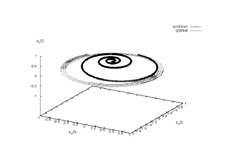
Figure 7: Implementation of the Z-gate with ${\bf p}_{I}=(0,1,0)^{T}$ and ${\bf p}_{d}=(0,-1,0)^{T}$. The 3-dimensional plot of the the Bloch vector ${\bf p}=\left(p_{x},p_{y},p_{z}\right)^{T}$ for undriven case and for driven by the optimal control field obtained by the conjugate gradient method is presented. Parameters as in Fig. 1.

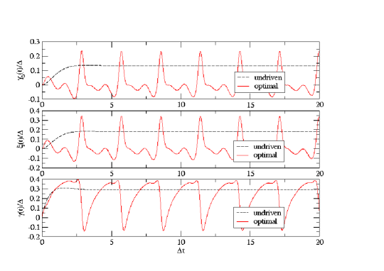
Figure 8: Implementation of the Z-gate with ${\bf p}_{I}=(0,1,0)^{T}$ and ${\bf p}_{d}=(0,-1,0)^{T}$. Depicted are the decay rate $\gamma$, the Lamb shift $\xi$ and the inhomogeneous term $\gamma_{0}$ as a function of time for undriven case and driven by the optimal control field selected by the conjugate gradient method. (a), (b) and (c) show, respectively, the results for $\gamma_{0}$, $\xi$ and $\gamma$. Parameters as in Fig. 1.

For the two examples of implementing a quantum Z-gate, The conjugate gradient method selects a ”multi–component low–frequency”. This aspect of the optimal control field is remarkable. Firstly, the optimum field is a superposition of harmonics. This allows one to identify rather small number of optimization parameters for a direct optimization scheme, such as a genetic code. Secondly, all essential frequency components lie below the the Ohmic cut–off frequency $\omega_{c}=20\Delta$. Hence, we have shown that there are optimized solutions for decoupling system from environment at lower frequence than required in the “bang–bang” approach.

The presented solutions was obtained by starting from control field zero and the optimization algorithm obtained, within the specified cost functional, a solution which performs 7 switching operations. In principle, one switching operation would be sufficient. Due to the possibility to dynamically create stable intermediate states one is in a similar position as with transferring an electron in an isolated two level system. In the latter case, increasing the intensity of a resonant harmonic light field induces an increasing number of Rabi flip operations.

V.2 Trapping

In the following two examples we study the control of the z–component of the Bloch vector, physically, corresponding to the spin direction or relative population of ”up” and ”down” states. First we consider trapping of the system in the excited state ${\bf p}_{d}=(0,0,1)$. $p_{x}=p_{y}=0$ at the initial time ensures that the Bloch vector has vanishing x– and y–component in the future, regardless of the control field applied. The problem becomes one–dimensional in the Bloch–vector space. The chosen cost functional is

$$J=\frac{1}{2t_{F}}\int_{0}^{t_{F}}dt\,\|{\bf p}(t)-{\bf p}_{d}\|^{2}$$ (92)

In this case, the running cost functional follows as ${\mathcal{L}}\left({\bf p}(t),{\mbox{\boldmath$\varepsilon$}}(t)\right)=\frac{1}{2t_{F}}\|{\bf p}(t)-{\bf p}_{d}\|^{2}$ and the final cost functional $\Phi\left[{\bf p}(t_{F})\right]$ is equal to zero. For the isolated two–level system there are several known ways of trapping a two–level system by an external control with $\sigma_{z}$–coupling. One can make the trapping state to the ground state of the system or one can apply a monochromatic high–frequency field with matched intensity to induce dynamic localization Grossmann . These strategies can be generalized and be applied to the dissipative two–level system Grifoni ; Stockburger . Both strategies have in common that one tries to find a control field which makes the trapping–state to an element of the decoherence–free subspace of the driven system. Following the first strategy, a static control field can be found to make the state ${\bf p}=(0,0,p_{z})^{T}$ for $-1\leq p_{z}\leq+1$ to the thermal equilibrium ground state of the driven system for given finite temperature. Alternatively, a high–frequency field can be used to dynamically decouple the open quantum system from the bath. In the “bang–bang” method mentioned in the introduction, this is achieved with a control field whose frequency is (much) higher than the maximum frequency of the bath Viola_1 ; Viola_2 ; Stigmunt_1 ; Jirari_2 . In the present model this is the phonon cut–off frequency $\omega_{c}$. Here we will show that a dynamic decoupling can be achieved by a field whose characteristic angular frequencies lie below $\omega_{c}$.

In the present model, an oscillating control field leads to a rapidly oscillating integrand for $\gamma(t)$ and $\gamma_{0}(t)$ leading to small values for these two functions. Fig. 9(d) shows the time evolution of $p_{z}$. The dotted line shows the free evolution of the system into its thermal–equilibrium ground state within a time of about $20/\Delta$. Starting from a guess for the control field in form of a Gaussian pulse, an optimized solution is obtained via the conjugate gradient method which stabilizes the system in state ${\bf p}=(0,0,1)^{T}$ rather well. Comparing, the initial guess to the selected optimal control field one sees in Fig. 9(a) that the oscillations of the Gaussian pulse get picked up and are amplified. In regions were the Gaussian factor suppressed the field the selected optimal field is less structured. Fig. 10 shows the power spectrum of original guess and the selected optimal control field. The main peak from the original guess gets amplified and higher harmonics of the central frequency of the original guess are used to fine tune the control field. The selected field still shows clear features of the original guess. This is quite typical for solutions obtained within the conjugate gradient method when more than one solution exists. Figs. 9(b) and (c) show that state trapping is indeed caused by dynamic decoupling in this case. $\gamma(t)$ and $\gamma_{0}(t)$ show high frequency oscillations of small amplitude about zero.

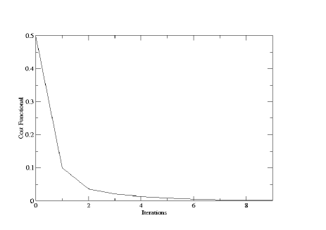
Figure 11: Trapping the system in an unstable quantum state i.e ${\bf p}(t)=(1,0,0)^{T}$ for all $t\in[0,t_{F}]$. Shown is the cost functional vs. the number of iterations. Parameters as in Fig. 9.

To address the issue of convergence of the numerical procedure we show the cost functional (92) versus the number of iterations in Fig. 11. It can be seen that, starting from a mediocre guess, convergence is reached typically within 10 iterations. Moreover, convergence is strictly monotonic. Compared to direct approaches, such as a genetic code, this method requires significantly lower number of computations of the cost functional and significantly less computation time. Thus the investment of setting up the optimization scheme by introducing the co–state and the extra task of backward integration for the latter pays off in the end. Moreover, the present method makes feasible the selection of ”arbitrary” optimized control fields, ı. e. an optimization of the control field at every mesh point in time. Due to the large number of mesh points this would make a direct optimization approach computationally highly expensive. There are, however, non–linear programming approaches which may fair well for the present system  Betts .

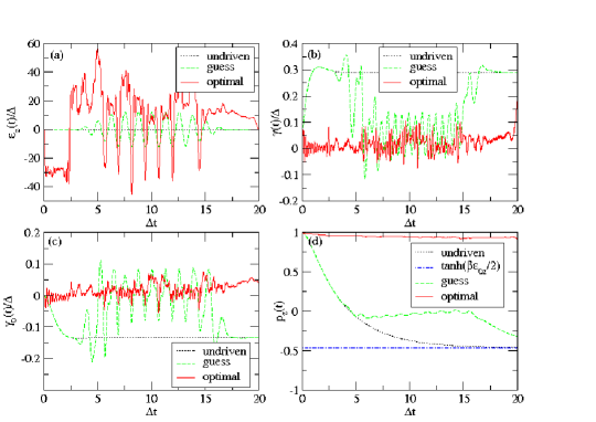
Figure 9: Trapping the system in an unstable quantum state, i.e, ${\bf p}(t)=(1,0,0)^{T}$ for all $t\in[0,t_{F}]$. Depicted are the control field $\varepsilon_{z}$, the decay rate $\gamma$, the inhomogeneous term $\gamma_{0}$ and the relative population $p_{z}$ as a function of time for three cases of undriven, driven by an harmonic field with a Gaussian shape (the guessed control field) and driven by the optimal control field selected by the conjugate gradient method. (a) shows the results for the control field $\varepsilon_{z}$, (b) and (c) show, respectively, the results for $\gamma$ and $\gamma_{0}$ while (d) show the results for $p_{z}$. The parameters used are $\alpha=0.2$, $\varepsilon_{0z}=-\Delta$, $\omega_{c}=20\Delta$ and $k_{B}T=\beta^{-1}=\hbar\Delta$. The final time is set as $t_{F}=20/\Delta$ and the chosen time step is $10^{-2}/\Delta$ corresponding to $M=2\times 10^{3}$ mesh points, i.e, the dimension of the optimal control problem.

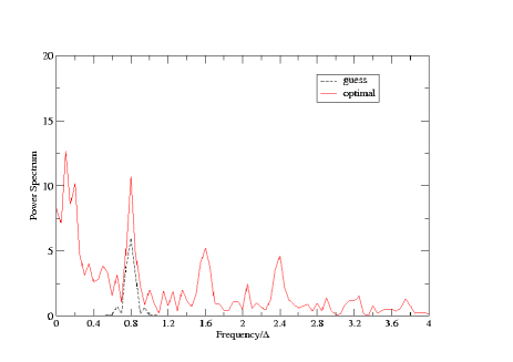
Figure 10: Trapping the system in an unstable quantum state i.e ${\bf p}(t)=(1,0,0)^{T}$ for all $t\in[0,t_{F}]$. Depicted is the comparison of the power spectrum of the optimal control field selected by the conjugate gradient method with the power spectrum of the guessed control field. Parameters as in Fig. 9.

V.3 Inversion of population

As a final example we consider the task of driving the system from its thermal equilibrium state $(0,0,p_{z})$ into the pure ”up” state $(0,0,1)$ and subsequent trapping in this state. The general cost functional given by Eq. (71) is adapted to the present task by setting

$$\Phi\left[{\bf p}(t_{F})\right]=\frac{w_{1}}{2}\|p_{z}(t_{f})-p_{zd}(t_{f})\|^{2}$$ (93)

and

$${\mathcal{L}}\left({\bf p}(t),{\mbox{\boldmath$\varepsilon$}}(t)\right)=\frac{w_{2}}{2t_{f}}\|p_{z}(t)-p_{zd}(t)\|^{2}\ +\frac{1}{2}s(t)\varepsilon^{2}(t)~{}~{}.$$ (94)

$s(t)$, $w_{1}$ and $w_{2}$ with $w_{1}+w_{2}=1$ are real-valued weight factors to specify driving ($w_{1}=1$) and trapping ($w_{2}=1$). One can use the latter two to shift significance between driving into a target state and driving the system along a specified trajectory $p_{zd}(t)$. The function $s(t)$ may be used to tailor the control pulse shape. In case of certain linear control problems the third term is necessary to make the problem regular Krotov . $-1\leq p_{zd}(t)\leq+1$ defines the “desired” trajectory of the system. For the present discussion we set $p_{zd}(t)=1$.

Numerical results are shown in Fig. (12). Let us first look at the undriven case for an initial state $(0,0,1)$, displayed by the dotted lines. It is seen in Fig. (12)(d) that, on the time scale considered, there is rapid thermalization of the system into the equilibrium state at about $(0,0,-0.96)$. Except for oscillations at very short times, $\gamma(t)$ and $\gamma_{0}(t)$ are essentially constant in time.

For the driven case we consider two situations. In the first we wish to prepare the system in the target state $(0,0,1)$ at $t_{F}=500$ when the system initially is in the thermal equilibrium state $(0,0,-0.964)$. We set $w_{1}=1$ and $w_{2}=0$. Since the intrinsic time scale is faster than the target time there exist many solutions to achieve the task. Here we choose an initial guess in form of a harmonic field of low frequency (adiabatic solution) and optimize this guess subsequently with the conjugate gradient method using 300 mesh points for the control field. We use $s(t)$ to suppress the control field at times around zero, as well as high intensities. Results for an optimal solution are shown by the solid lines in Fig. (12). The selected optimal control fulfils the conditions imposed and leads to a gradual transition into the target state. In this particular case, the qubit–environment coupling has effectively been reduced over the undriven case.

The second case considered is driving the system from its thermal equilibrium state into the target state $(0,0,1)$ as fast as possible and subsequently trap it there. In the cost functional we set $w_{1}=0$ and $w_{2}=1$. Again a low–frequency harmonic field is selected for the initial guess and $s(t)$ is used to tailor the selected control field at times around zero, as well to limit its intensity. The results are shown by the dashed lines in Fig. (12). The selected control field rises sharply from about zero to, essentially, a plateau. $\gamma(t)$ and $\gamma_{0}(t)$ vary significantly only in the time during the transfer. Although high fields are suppresses around time zero, the selected optimal control field manages a more rapid transfer into the new equilibrium case (dashed line in Fig. (12)(d)) than the undriven case (dotted line in Fig. (12)(d)). Hence, we show that we have been able to significantly increase the effective interaction strength.

VI SUMMARY AND CONCLUSIONS

In this work we have presented dynamic control of open quantum systems as an optimization problem. The Bloch–Redfield approach was used to derive Markovian kinetic equations of a driven open quantum system whereby the external control was treated non–perturbatively. This approach leads to a Redfield tensor which accounts for a coupling between system and bath which contains a causal dependence upon the external control field. Indeed, the present approach is equivalent to the time–convolutionless projection operator method within second order in the system–environment coupling Breuer . This control–field dependence of the effective system interaction allows steering of the open quantum system and its coupling to its environment beyond what is feasible within a semiclassical treatment of the environment in which interference between the system–control–field interaction and the system–environment interaction is neglected Jirari .

This approach was applied to the spin–boson model in the strong electron–boson coupling limit. Using the polaron transformation, the kinetic equations for the Bloch vector were derived and analysed. They feature an effective coupling in the spin system which is renormalized by the spin–phonon interaction and displays a causal dependence (non–local in time) on the control field. Analytic results for Lamb shift and decay time are presented for the zero temperature limit in the absence of the control. It is shown for several examples that both the stationary states of the driven open quantum system and the rates at which they are reached can be controlled to a large degree.

Steering of the open quantum system is formulated and solved as an optimization problem via Pontryagin’s minimum principle which is based on the introduction of Lagrangean multipliers in form of a co–state (adjoint state). The set of optimality conditions is solved iteratively using a conjugate gradient method. Numerical examples show that it leads to a monotonic improvement in the cost functional.

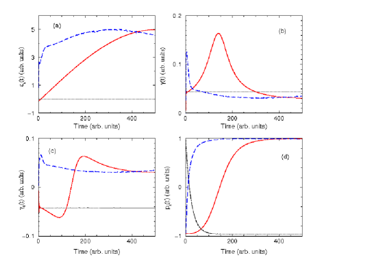
Figure 12: Control of relative population $p_{z}(t)$: (a) shows the selected control field, (b) shows $\gamma(t)$, (c) shows $\gamma_{0}(t)$ and (d) shows the corresponding time evolution. The dotted lines are for $\varepsilon(t)$ =0 (undriven case), the solid line is for transfer from $(0,0,-0.965)$ to $(0,0,1)$, and the dashed lines are for transfer to and trapping in $(0,0,1)$. The parameters used are $\alpha=0.25$, $\varepsilon_{0z}=-2$, $\Delta=0.5$, $\omega_{c}=10$, $t_{F}=500$, and temperature $\beta^{-1}=0.5$.

Several physical situations have been investigated numerically to demonstrate quantum–interference–based optimal control of open quantum system. The studies of a $\pi$ rotation of the Bloch vector in the x–y plane and trapping along the z–axis have shown that optimal control fields of moderate frequency (as compared to the phonon cut–off frequency) can be selected which significantly extend the lifetime of purity and, hence, improve the chance of successful completion of an error free quantum operation or the storage of a dissipative system in a fixed quantum state. The analysis of driving and subsequent trapping into a quantum state, which for the undriven system is highly unstable, at the example of population transfer has shown that this task can be achieved by slowly varying fields for the present model. Moreover, the rate of transfer can be varied within limits set by the maximally obtainable effective coupling strength of the open quantum system. The latter is determined by the system, the environment, and the system–environment coupling.

This analysis has also shown that the inverse problem of identification of optimal control fields in general has a large number of optimal solutions. Within the conjugate gradient method the selected optimal solutions usually show a remnance of the initial guess. The number of optimal solutions may be reduced by additional constraints which may be used to select experimentally feasible solutions, such as fields with a gradual rise time, rather than abruptly turned on fields. In some cases, quite different fields can produce near equal results. For example, trapping in a quantum state may be obtained by applying a static control field which makes the trapping state to its (approximate) new ground state. In this case a decoupling of the system–environment interaction is not necessary or even desirable. It is in fact the system–bath coupling which drives the system system into its new equilibrium state. As an important result this study has shown that state–specific optimal control can be achieved by time–dependent fields whose characteristic frequencies lie below the maximum characteristic bath frequency. Alternatively, high–frequency high–amplitude “bang–bang” control fields, reminiscent of the effect of dynamic localization, may induce dynamic decoupling by making the effective coupling strength small.

Optimization of a dissipative quantum gate poses a more complicated problem than the one addressed here since optimization should occur independent of the input state Cirac ; Thorwart . Moreover, the output state (target state), in general, depends on the input state. We find that an optimal control field critically depends on the input state. A bang–bang solution (which is probably difficult to implement in experiment) can be envisioned whereby a high–frequency high–intensity field is applied to suppress the effective system–environment coupling. However, such a field usually also has a direct coupling channel to the system which may cause problems when the control field is not perfectly suitable for the input state. Whether the present approach which is based on specific trajectories can be extended to optimize quantum gates by some averaging procedure or whether an optimization should directly be aimed at the superoperator responsible for the time–evolution will require further investigation.

Appendix A SCHWINGER AND FEYNMAN REPRESENTATIONS

The Schwinger and Feynman representations Peskin will play an important role in the determination of the decay rate and the Lamb shift (see below).

The Schwinger representation involves the Euler Gamma function defined by

$${\bf\Gamma(\nu)}=\int_{0}^{\infty}\,dt\,e^{-t}\,t^{\nu-1},\qquad{\rm Re}\,\nu>0,$$ (95)

Making the variable change $Du=t$ in the definition of the Euler gamma function (95), leads to

$$\frac{1}{D^{\nu}}=\frac{1}{{\bf\Gamma(\nu)}}\int_{0}^{\infty}\,du\,u^{\nu-1}e^{-uD},\quad\,{\rm Re}\,\nu>0\quad{\rm Re}\,D>0.$$ (96)

The identity (96) allows to write the denominators $D$ of the propagator in form of an integral on the Schwinger parameter $u$.

On the other hand the Feynman representation Peskin introduces a parameter $x$ (Feynman parameter) to squeeze the denominator factors into a single polynomial form

$$\frac{1}{A\centerdot B}=\int_{0}^{1}\,dx\,\left[Ax+B(1-x)\right]^{-2}\,.$$ (97)

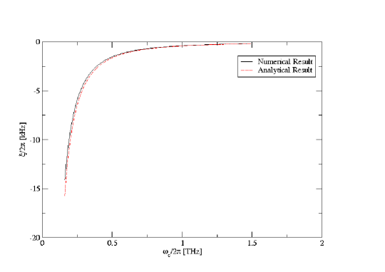
Figure 13: The Lamb shift for the undriven case and zero temperature as a function of the Ohmic cutoff frequency $\omega_{c}$. The test of our analytical result, Eq. (116), by comparison of a direct numerical integration of Eq. (C) is shown. The parameters used are the coupling $\alpha=1.2$, the tunnel amplitude $\frac{\Delta}{2\pi}=635\,\mbox{MHz}$ and the energy bias $\frac{\varepsilon_{0z}}{2\pi}=560\,\mbox{MHz}$.

Appendix B DERIVATION OF THE DECAY AT ZERO TEMPERATURE

Here we derive an analytical expression of the decay rates

$$\gamma(\varepsilon_{0z}) = \Delta^{2}\int_{0}^{\infty}\,d\tau\,e^{-Q_{2}(\tau)}\cos[Q_{1}(\tau)]\cos[\varepsilon_{0z}\tau]$$ (98)

$$= \gamma_{f}(\varepsilon_{0z})+\gamma_{b}(\varepsilon_{0z})\,,$$

with

$$\gamma_{f}(\varepsilon_{0z})=\frac{\Delta^{2}}{2}{\rm Re}\int_{0}^{\infty}\,d\tau\,e^{-Q_{2}(\tau)}e^{iQ_{1}(\tau)}e^{-i\varepsilon_{0z}\tau}\,,$$ (99)

and

$$\gamma_{b}(\varepsilon_{0z})=\frac{\Delta^{2}}{2}{\rm Re}\int_{0}^{\infty}\,d\tau\,e^{-Q_{2}(\tau)}e^{iQ_{1}(\tau)}e^{i\varepsilon_{0z}\tau}$$ (100)

are, respectively, the forward and the backward decay rates. Note that $\gamma_{b}(\varepsilon_{0z})=\gamma_{f}(-\varepsilon_{0z})$. Substituting Eqs. (53a) and (55) into Eq. (99), we obtain

$$\gamma_{f}(\varepsilon_{0z})=\frac{\Delta^{2}}{2}{\rm Re}\int_{0}^{\infty}\frac{e^{-i\varepsilon_{0z}\tau}}{{(1-i\omega_{c}\tau)}^{2\alpha}}\,d\tau\,.$$ (101)

Now with the help of the Schwinger identity (96), Eq. (101) can be written as

$$\gamma_{f}(\varepsilon_{0z})=\frac{\Delta^{2}}{2{\bf\Gamma}(2\alpha)}{\rm Re}\int_{0}^{\infty}du\,u^{2\alpha-1}\,e^{-u}\,\int_{0}^{\infty}d\tau e^{-i(\varepsilon_{0z}-u\omega_{c})\tau}\,.$$ (102)

Using the fact that

$$\int_{0}^{\infty}d\tau e^{-i(\varepsilon_{0z}-u~{}\omega_{c})\tau}=\pi\,\delta(\varepsilon_{0z}-u~{}\omega_{c})-i~{}\mbox{PP}\left(\frac{1}{\varepsilon_{0z}-u\omega_{c}}\right)\,,$$ (103)

where the first term is the Dirac distribution and the second term PP denotes the Cauchy principal part of the integral $\int_{0}^{\infty}d\tau/\left(\varepsilon_{0z}-u\,\omega_{c}\right)$ and introducing the Heaviside distribution $\theta(u)$ to extend the bounds of integration from $-\infty$ to $+\infty$, Eq. (102) becomes

$$\gamma_{f}(\varepsilon_{0z})=\frac{\pi\Delta^{2}}{2{\bf\Gamma}(2\alpha)\,\omega_{c}}\int^{+\infty}_{-\infty}du\,u^{2\alpha-1}\,e^{-u}\,\theta(u)\,\delta\left(u-\frac{\varepsilon_{0z}}{\omega_{c}}\right)\,.$$ (104)

Evaluating the convolution product (104), one ends up with the following formula:

$$\gamma_{f}(\varepsilon_{0z})=\frac{\pi\Delta^{2}}{2{\bf\Gamma}(2\alpha)}\left(\frac{1}{\omega_{c}}\right)^{2\alpha}\,\varepsilon^{2\alpha-1}_{0z}\,e^{-\left(\varepsilon_{0z}/\omega_{c}\right)}\,\theta\left(\varepsilon_{0z}/\omega_{c}\right)\,.$$ (105)

The Heaviside distribution (or step function), insures that at zero temperature absorption of energy from the environment is not possible. The final result for the decay rate is then for $\alpha>\frac{1}{2}$,

$$\gamma(\varepsilon_{0z}>0) = \frac{\pi\Delta^{2}}{2{\bf\Gamma}(2\alpha)}\left(\frac{1}{\omega_{c}}\right)^{2\alpha}\varepsilon^{2\alpha-1}_{0z}\,e^{-\left(\varepsilon_{0z}/\omega_{c}\right)}\,,$$ (106a)

$$\gamma(\varepsilon_{0z}<0) = \frac{\pi\Delta^{2}}{2{\bf\Gamma}(2\alpha)}\left(\frac{1}{\omega_{c}}\right)^{2\alpha}\left(-\varepsilon_{0z}\right)^{2\alpha-1}\,e^{\left(\varepsilon_{0z}/\omega_{c}\right)}.$$

For the inhomogeneous term

$$\gamma_{0}(\varepsilon_{0z})=\Delta^{2}\int_{0}^{\infty}\,d\tau\,e^{-Q_{2}(\tau)}\sin[Q_{1}(\tau)]\sin[\varepsilon_{0z}\tau]\,,$$ (107)

similar calculation of the decay rate leads for $\alpha>1/2$ to

$$\gamma_{0}(\varepsilon_{0z}>0) = \frac{\pi\Delta^{2}}{2{\bf\Gamma}(2\alpha)}\left(\frac{1}{\omega_{c}}\right)^{2\alpha}\varepsilon^{2\alpha-1}_{0z}\,e^{-\left(\varepsilon_{0z}/\omega_{c}\right)}\,,$$ (108a)

$$\gamma_{0}(\varepsilon_{0z}<0) = -\frac{\pi\Delta^{2}}{2{\bf\Gamma}(2\alpha)}\left(\frac{1}{\omega_{c}}\right)^{2\alpha}\left(-\varepsilon_{0z}\right)^{2\alpha-1}\,e^{\left(\varepsilon_{0z}/\omega_{c}\right)}.$$

At zero temperature, the detailed balance condition takes the following form

$$\frac{\gamma_{0}(\varepsilon_{0z})}{\gamma(\varepsilon_{0z})}=\left\{\begin{array}[]{cc}1&\quad\mbox{if}\quad\varepsilon_{0z}>0\\ -1&\quad\mbox{if}\quad\varepsilon_{0z}<0\end{array}\right.$$ (109)

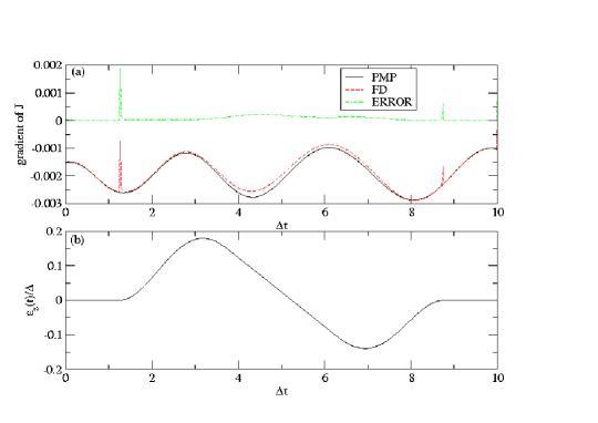
Figure 14: Implementation of the Z-gate with ${\bf p}_{I}=(1,0,0)^{T}$ and ${\bf p}_{F}=(-1,0,0)^{T}$. The upper panel (b) shows the numeric comparison between Pontryagin’s minimum principle (PMP) and the finite difference (FD) approximation for computing the gradient of the final cost functional in Eq. (88) evaluated at the control field displayed in the lower panel (b). The parameters used are $\alpha=0.2$, $\varepsilon_{0z}=\Delta$, $\omega_{c}=20\Delta$, $k_{B}T=\beta^{-}1=\hbar\Delta$. The final time is set as $t_{F}=10/\Delta$ and the chosen time step is $5\times 10^{-2}\Delta$ corresponding to $M=2\times 10^{2}$ mesh points, i.e, the dimension of the optimal control problem.

Appendix C DERIVATION OF THE LAMB SHIFT AT ZERO TEMPERATURE

Let us now compute the Lamb shift given by

$$\xi(\varepsilon_{0z})=\Delta^{2}\int_{0}^{\infty}d\tau\,e^{-Q_{2}(\tau)}\cos[Q_{1}(\tau)]\sin[\varepsilon_{0z}\tau]$$

$$=\frac{\Delta^{2}}{2}{\rm Im}\int_{0}^{\infty}d\tau e^{-Q_{2}(\tau)}\left\{e^{iQ_{1}(\tau)}e^{i\varepsilon_{0z}\tau}+e^{-iQ_{1}(\tau)}e^{i\varepsilon_{0z}\tau}\right\}\,.$$

Substituting Eqs. (53a) and (55) into Eq. (C) and using (103), we obtain

$$\xi(\varepsilon_{0z})=-\frac{\Delta^{2}}{{\bf\Gamma}(2\alpha)}\frac{\varepsilon_{0z}}{\omega^{2}_{c}}\int_{0}^{\infty}\,du\frac{u^{2\alpha-1}\,e^{-u}}{u^{2}-\left(\frac{\varepsilon_{0z}}{\omega_{c}}\right)^{2}}\,,$$ (111)

where $u$ is the dimensionless Schwinger parameter. The last integral can not be computed using the residues theorem since it is singular at $u=\pm\frac{\varepsilon_{0z}}{\omega_{c}}$ and at $u=0$ when $\alpha<1/2$.

Nevertheless the application of the Feynman identity (97) to Eq. (111), leads to

$$\xi(\varepsilon_{0z})=-\frac{\Delta^{2}}{{\bf\Gamma}(2\alpha)}\frac{\varepsilon_{0z}}{\omega^{2}_{c}}\int_{0}^{1}\,dx\,{\mathcal{I}}\left(x,\alpha,\frac{\varepsilon_{0z}}{\omega_{c}}\right)\,,$$ (112)

with

$${\mathcal{I}}\left(x,\alpha,\frac{\varepsilon_{0z}}{\omega_{c}}\right)=\int_{0}^{\infty}\,du\frac{u^{2\alpha-1}\,e^{-u}}{\left(u+(2x-1)\frac{\varepsilon_{0z}}{\omega_{c}}\right)^{2}}$$ (113)

which after the change variable $v=u+(2x-1)\frac{\varepsilon_{0z}}{\omega_{c}}$ is transformed to

$${\mathcal{I}}\left(x,\alpha,\frac{\varepsilon_{0z}}{\omega_{c}}\right) = \int_{(2x-1)\frac{\varepsilon_{0z}}{\omega_{c}}}^{\infty}\,dv\left(v-(2x-1)\frac{\varepsilon_{0z}}{\omega_{c}}\right)^{2\alpha-1}$$ (114)

$$\quad\quad\quad\times v^{-2}e^{-v}\,e^{(2x-1)\frac{\varepsilon_{0z}}{\omega_{c}}}\,.$$

Now, the approximation $\frac{\varepsilon_{0z}}{\omega_{c}}\ll 1$ leads to

$${\mathcal{I}}\left(x,\alpha,\frac{\varepsilon_{0z}}{\omega_{c}}\right) = e^{(2x-1)\frac{\varepsilon_{0z}}{\omega_{c}}}\,\int_{0}^{\infty}\,dv\,v^{2\alpha-3}\,e^{-v}$$ (115)

$$= e^{(2x-1)\frac{\varepsilon_{0z}}{\omega_{c}}}\,{\bf\Gamma}(2\alpha-2)\,.$$

Using Eq. (115), we get from (112) for $\alpha>1$

$$\xi(\varepsilon_{0z})=-\frac{\Delta^{2}}{\omega_{c}^{2}}\,\varepsilon_{0z}\,\frac{\sinh\left(\varepsilon_{0z}/\omega_{c}\right)}{\left(\varepsilon_{0z}/\omega_{c}\right)}\,\frac{{\bf\Gamma}(2\alpha-2)}{{\bf\Gamma}(2\alpha)}\,.$$ (116)

Combining again the Schwinger identity (96) with Eq. (115) and after some algebra we obtain for $\frac{1}{2}<\alpha<1$

$$\xi(\varepsilon_{0z})=-\frac{\Delta^{2}}{2}\frac{\varepsilon_{0z}}{\omega^{2}_{c}}\,\left({\frac{\varepsilon_{0z}}{\omega_{c}}}\right)^{2\alpha-2}{\bf\Gamma}(2-2\alpha)\,\frac{1}{2\alpha-1}$$

$$\quad\quad\quad\quad\times\lim_{\eta\to 0}\left(1-e^{(2\alpha-1)\log(2\eta-1)}\right)\,.$$ (117)

A such limit in the last equation does not exist.

I summary, our prediction for the renormalization of the energy bias due to the Lamb shift at zero temperature; in leading order in $\frac{\varepsilon_{0z}}{\omega_{c}}$ ($\frac{\varepsilon_{0z}}{\omega_{c}}\ll 1$) and in strong coupling regime ($\alpha>1$), is the following:

$$\tilde{\varepsilon}_{0z}=\varepsilon_{0z}\times\left[1-\frac{\Delta^{2}}{\omega_{c}^{2}}\,\frac{\sinh\left(\varepsilon_{0z}/\omega_{c}\right)}{\left(\varepsilon_{0z}/\omega_{c}\right)}\,\frac{{\bf\Gamma}(2\alpha-2)}{{\bf\Gamma}(2\alpha)}\right]\,.$$ (118)

The agreement of the analytical expression for the Lamb shift, Eq. (116), with the numerical integration of Eq. (C) by Gauss quadrature is shown in Fig.(13).

Appendix D NUMERICAL TEST OF THE GRADIENT

In order to test the method of Pontryagin’s minimum principle (PMP) given by Eq. (IV.3) to compute the gradient of the cost functional, Eq. (88), we compare it with the finite difference approximation (FD). Fig. 14 shows the result of the gradient for a control field of the form $\varepsilon_{z}(t)=A(t)\cos(\Omega t+\phi)$ with frequency $\Omega$, phase $\phi$, and a Gaussian envelope $A(t)$. We can see in Fig. 14 that the error, $\mbox{ERROR}=\left|\nabla^{\rm PMP}J-\nabla^{\rm FD}J\right|,$ is roughly zero except at the switching times of the control field where its amplitude is suddenly increased. The good agreement observed for this case occurs because the frequency $\Omega=10^{-1}\times\Delta$ of the control field is low and causes a slow variation of the cost functional. In this case the finite difference approximation is numerically stable and gives good results compared to the adjoint–state method. In case of high control field, this good agreement is lost because the cost functional varies very rapidly and renders the finite difference method numerically unstable.

References

- (1) M. A. Nielson and I. L. Chuang, Quantum Computation and Quantum Information (Cambridge University Press, Cambridge, UK, 2000).
- (2) W. G. Unruh, Phys. Rev. A 51, 992 (1995)
- (3) P. Zanardi and M. Rasetti, Phys. Rev. Lett. 79, 3306 (1997).
- (4) D. A. Lidar, I. L. Chuang and K. B. Whaley, Phys. Rev. Lett. 81, 2594 (1999).
- (5) J. Preskill, Proc. Roy. Soc. Lond. A454, 385 (1998).
- (6) E. Knill E, R. Laflamme and L. Viola, Phys. Rev. Lett. 84, 2525 (2000).
- (7) J. Wang J and H. Wiseman, Phys. Rev. A 64, 063810 (2001).
- (8) L. Viola and S. Lloyd, Phys. Rev. A 58, 2733 (1998).
- (9) L. Viola, E. Knill, and S. Lloyd, Phys. Rev. Lett. 82, 2417 (1999); 83, 4888 (1999); 85, 3520 (2000).
- (10) P. Zanardi, Phys. Lett. A 258, 77 (1999).
- (11) D. Vitali and P. Tombesi, Phys. Rev. A 59, 4178 (1999); 65, 012305 (2001).
- (12) C. Uchiyama and M. Aihara, ibid. 66, 032313 (2002).
- (13) M. S. Byrd and D. A. Lidar, Quantum Inf. Process. 1, 19 (2002); Phys. Rev. A 67, 012324 (2003).
- (14) V. Protopopescu, R. Perez, C. D’Helon, and J. Schmulen, J. Phys. A: Math. Gen. 36, 2175 (2003).
- (15) Wayne. M. Itano and al., Phys. Rev. A 41, 2295 (1990).
- (16) P. Facchi, S. Tasaki, S. Pascazio, H. Nakazato, A. Tokuse, and D. A. Lidar, Phys. Rev. A 71, 022302 (2005)
- (17) L. Viola, J. Mod. Opt. 51, 2357 (2004).
- (18) X. Hu and W. Pötz, Phys. Rev. Lett. 82, 3116 (1999).
- (19) H. Jirari and W. Pötz, Phys. Rev. A 72, 013409 (2005).
- (20) O. Kocharovskaya et al., Phys. Rev. A 49, 4928 (1994).
- (21) D. H. Schirrmeister and V. May, Chem. Phys. Lett. 297, 383 (1998).
- (22) R. Xu at al., J. Chem. Phys. Lett. 120, 6600 (2004).
- (23) M. Morillo, C. Denk and R. I. Cukier, Chem. Phys. 212, 157 (1996).
- (24) M. Morillo and R. I. Cukier, Phys. Rev. B 54, 13962 (1996).
- (25) Yu. Dakhnovskii, Phys. Rev. B 49 (1994);
- (26) M. Grifoni and P. Hänggi, Phys. Rep 304, 1 (1998).
- (27) K. M. Fonseca Romero, S. Kohler and P. Hänggi, Chem. Phys. 296, 307 (2004);
- (28) K. M. Fonseca Romero, S. Kohler and P. Hänggi, Phys. Rev. Lett. 95 , 140502 (2005).
- (29) H. Jirari and W. Pötz, e-print cond-mat/0506379; Submitted to Europhysics Letters.
- (30) L. S. Pontryagin, The Mathematical Theory of the Optimal Process (Wiley-Interscience, New York, 1962).
- (31) A. E. Bryson, Y. C. Ho, Applied Optimal Control, Hemisphere, New York, 1975.
- (32) J. T. Betts, Practical methods for Optimal Control using Nonlinear Programming (SIAM, Philadelphia 2001).
- (33) U. Weiss, Quantum Dissipative Systems, (World Scientific, Singapore 1999).
- (34) G. D. Mahan, Many Particles Physics, (Plenum Press, New York, 1999).
- (35) B. Krummheuer, V.M. Axt, and T. Kuhn, Phys. Rev. B. 65, 195313 (2002).
- (36) U. Hohenester and G. Stadler, Phys. Rev. Lett 92, 196801 (2004).
- (37) J. Zhang and W. Pötz, Phys. Rev. B 48, 11583 (1993).
- (38) I. Rousochatzakis, Y. Ajiro, H. Mitamura, P. Kögerler and M. Luban, Phys. Rev. Lett 94, 147204 (2005); I. Rousochatzakis and M. Luban e-print cond-mat/0503695.
- (39) A. E. Allahverdyan, R. S. Garcià and Th. M. Nieuwenhuizen, Phys. Rev. Lett. 93, 260404 (2005).
- (40) Yu. Makhlin, G. Schön and A. Schnirman, Rev. Mod. Phys. 73, 357 (2001).
- (41) A. J. Leggett, S. Chakravarty, A. T. Dorsey, M. P. A. Fisher, A. Garg and W. Zwerger, Rev. Mod. Phy 59, 1 (1987).
- (42) H. P. Breuer and F. Petruccione, The Theory of Open Quantum Systems (Oxford University Press 2002).
- (43) K. Blum, Density Matrix Theory and Applications., 2nd Edition (Plenum Press, New York, 1996).
- (44) L. Hartmann, I. Goychuk, M. Grifoni and P. Hänggi, Phy. Rev. E 61, R4687 (2000).
- (45) H. Risken, The Fokker-Planck Equation, 2nd Edition (Springer-Verlag, Berlin, Heidlberg, New York, 1989).
- (46) H. Grabert, Phys. Rev. B 46, 12753 (1992).
- (47) C. Aslangul, N. Pottier and D. Saint-James, J. Phys. (Paris) 47, 1657 (1986).
- (48) T. Vorrath and T. Brandes, Phys. Rev. Lett. 95, 070402 (2005).
- (49) J. F. Frédéric, J. Ch. Gilbert, C. Lemaréchal and C. Sagastizabál. Numerical Optimization: Theoretical and Practical Aspects (Springer, Heidelberg, 2003).
- (50) W. H. Press, S.A. Teukolsky, W. T. Vetterling and B. P. Flannery, Numerical Recipes, 2nd Edition (Cambridge University Press, Cambridge England, 1992).
- (51) http://www.netlib.org/port; D. M. Gay, Usage Summary for Selected Optimization Routines, Computing Science Technical Report No 153, ATT Bell Laboratories (1990).
- (52) F. Grossmann, T. Dittrich, P. Jung, and P. Hänggi, Phys. Rev. Lett 67 516 (1991).
- (53) J. Stockburger, Phys .Rev. E 59, R4709 (1999).
- (54) V. F. Krotov, Global Methods in Optimal Control Theory (Dekker, New York, 1996).
- (55) M. E. Peskin and D. V. Schroeder, An Introduction to Quantum Field Theory (Addison-Wesley, Reading, 1995).
- (56) J. F. Poyatos, J.J. Cirac, and P. Zoller, Phys. Rev. Lett. 78, 390 (1997).
- (57) M. Thorwart and P. Hänggi, Phys. Rev. A 65, 012309-1 (2001).