General up to next-nearest neighbour elasticity of triangular lattices
in three dimensions

Abstract

triangular lattice, lattice elasticity, non-central forces, cytoskeleton We establish the most general form of the discrete elasticity of a 2D triangular lattice embedded in three dimensions, taking into account up to next-nearest neighbour interactions. Besides crystalline system, this is relevant to biological physics (e.g., red blood cell cytoskeleton) and soft matter (e.g., percolating gels, etc.). In order to correctly impose the rotational invariance of the bulk terms, it turns out to be necessary to take into account explicitly the elasticity associated with the vertices located at the edges of the lattice. We find that some terms that were suspected in the litterature to violate rotational symmetry are in fact admissible.

1 Introduction

Since Born and von Kármán, the construction of microscopic elastic models of crystals has formed an important part of solid-state physics, aimed to determine elastic constants and lattice dynamical properties (Born & von Kármán 1912; Born 1914). Imposing global translational and rotational invariance is a delicate matter, although the required relationship are well established (Born & Huang 1954). In fact, inconsistencies associated with rotational invariance in the earlier models were pointed out by Lax (1965) and Keating (1966$a,b$). More recently, the importance of triangular lattices has emerged with the study of soft matter systems such as percolating gels (Feng & Sen 1984; Schwartz et al. 1985; Arbabi & Sahimi 1993), membrane with crystalline order (Kantor & Nelson 1987; Seung & Nelson 1988; Gompper & Kroll 1997), biological membranes (Discher et al. 1997; Coughlin & Stamenovic 2003), red blood cell cytoskeleton (Saxton 1990; Lim et al. 2002; Marcelli et al. 2005), and finite element modeling (Gusev 2004).

In this paper, we consider a triangular lattice embedded in three dimensions and we determine the most general expression of the harmonic elastic energy up to next-nearest neighbour interactions. We formulate a systematic procedure to generate all the energy terms allowed by symmetry. This procedure could be applied to other type of lattices. We show that in order to correctly ensure rotational invariance, it is necessary to consider the boundary of the lattice, as first suggested by Lax (1965). Our central result, equation (25), gives all the allowed energy terms, with no particular connection to mechanical elements such as springs, elastic wedges, etc. This contrasts with the above cited papers that postulate energy terms in a non exhaustive way. In particular, the most general energy contains a non-central nearest neighbour term (with coefficient $K_{t}$), which was believed to violate rotational invariance in percolating gels (Feng & Sen 1984) on the grounds of Keating’s argumentation (1966$a,b$). The situation is actually delicate since in a later paper, Keating (1968) restricted the generality of some assertions of its earlier papers.

Our paper is organised as follows. In §2 we formulate the elastic energy of triangular lattices. In §2 $a$, we write down all the scalar energy terms quadratic in the displacements of the lattice vertices. In §2 $b$, we retain only the terms satisfying the six-fold symmetry of an infinite triangular lattice. In §2 $c$, we consider also the edges: we study the symmetries relative to them and we retain the allowed edge terms. In §2 $d$, we impose global translational and rotational invariance, taking explicitely into account the reduced symmetry of the boundary, and we retain the allowed terms. In §2 $e$, we collect all the contributions and we extract the resulting bulk terms. In §3, we analyse and discuss the results obtained in §2. In §3 $a$, we give a possible interpretation of our energy in terms of mechanical elements. In §3 $b$, we rewrite the energy into the generic expression (25), which constitutes our central result. In §3 $c$, we establish the connection between our model and its continuum version. Finally, in §4, we give a brief summary and we detail the origin of the rotational invariance problem.

2 Discrete elasticity model

2.1 General definitions

Let us consider a bounded triangular lattice. In its undistorted state, we assume that it lies in a plane $\mathcal{P}$ and that its vertices (i.e. its sites) are evenly separated by a distance $\ell$ (figure 1). We denote by $\bm{r}^{\alpha}\in\mathcal{P}$ the position of a generic vertex $\alpha$. We also assume that the elastic properties of the lattice are symmetric with respect to $\mathcal{P}$.

In an arbitrary distorted state, $\bm{r}^{\alpha}$ becomes $\bm{r}^{\alpha}+\bm{u}^{\alpha}$, where $\bm{u}^{\alpha}$ is a three-dimensional displacement. The most general quadratic expansion of the lattice elastic energy, $F$, is given by

$$F\left(\left\{\bm{u}^{\alpha}\right\}\right)=\sum_{\alpha}\bm{u}^{\alpha}\cdot\bm{S}^{\alpha}\cdot\bm{u}^{\alpha}+\sum_{\alpha}\sum_{\beta\neq\alpha}\bm{u}^{\alpha}\cdot\bm{A}^{\alpha\beta}\cdot\bm{u}^{\beta}\,.$$ (1)

In this expression, we have separated the terms coupling identical vertices from those coupling different vertices. We have excluded the terms linear in $\bm{u}^{\alpha}$, because they must vanish for the undistorted state to be a minimum of the energy. Since $F$ is scalar, the tensors $\bm{S}^{\alpha}$ and $\bm{A}^{\alpha\beta}$ must satisfy $(\bm{S}^{\alpha})^{\mathrm{t}}=\bm{S}^{\alpha}$ and $(\bm{A}^{\alpha\beta})^{\mathrm{t}}=\bm{A}^{\beta\alpha}$, where the superscript t means transpose. Note that in general $\bm{A}^{\alpha\beta}\neq\bm{A}^{\beta\alpha}$.

We fix the interaction range by assuming that all the $\bm{A}^{\alpha\beta}$ vanish except when $\alpha$ and $\beta$ are nearest or next-nearest neighbours.

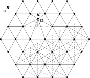
Figure 1: Triangular elastic lattice with the vertex $\alpha$ displaced by $\bm{u}^{\alpha}$. Nearest neighbours are indicated by plain lines and next-nearest neighbours by dashed lines (for clarity, the latters are drawn on one half of the figure only). The edge length is $N\ell$ with $N=3$.

2.2 Bulk terms

To begin with, we consider the bulk vertices, i.e. the vertices that are far away enough from the boundary (this point will be precised in §2$\,c$) so that the triangular symmetry may be assumed. In the bulk the elastic properties are assumed to be spatially homogeneous. Let $\bm{n}$ be a unitary vector normal to $\mathcal{P}$. Let ($\bm{t}_{1}$, $\bm{t}_{2}$) be two three-dimensional vectors forming a local orthonormal basis in $\mathcal{P}$, allowed to vary from site to site. The tensors $\bm{S}^{\alpha}$ and $\bm{A}^{\alpha\beta}$ can be decomposed into the complete basis $\mathcal{B}=(\bm{t}_{1}\otimes\bm{t}_{1},\,\bm{t}_{1}\otimes\bm{t}_{2},\,\bm{t}_{2}\otimes\bm{t}_{1},\,\bm{t}_{2}\otimes\bm{t}_{2},\,\bm{n}\otimes\bm{n})$, where the symbol $\otimes$ represent the tensorial product. Elements linear in $\bm{n}$, such as $\bm{t}_{1}\otimes\bm{n}$, have been excluded, since the undistorted lattice is symmetric with respect to $\mathcal{P}$.

To construct $\bm{S}^{\alpha}$, we take $\bm{t}_{1}$ along any one of the six nearest-neighbour directions of the undistorted lattice, and $\bm{t}_{2}=\bm{n}\times\bm{t}_{1}$. Because of the triangular symmetry, each term in the decomposition of $\bm{S}^{\alpha}$ must be even in $\bm{t}_{1}$ and in $\bm{t}_{2}$, and the coefficients of $\bm{t}_{1}\otimes\bm{t}_{1}$ and $\bm{t}_{2}\otimes\bm{t}_{2}$ must be equal (this condition is necessary for $\bm{S}^{\alpha}$ to be invariant under an in-plane $\frac{\pi}{3}$ rotation). Hence,

$$\bm{S}^{\alpha}=s_{1}\,\bm{I_{2}}+\tilde{s}_{1}\,\bm{n}\otimes\bm{n},$$ (2)

where $\bm{I_{2}}=\bm{t}_{1}\otimes\bm{t}_{1}+\bm{t}_{2}\otimes\bm{t}_{2}$ is the identity tensor in the plane $\mathcal{P}$. By virtue of the lattice homogeneity, the coefficients $s_{1}$ and $\tilde{s}_{1}$ should not depend on $\alpha$.

We now construct $\bm{A}^{\alpha\beta}$. Let $\bm{t}^{\alpha\beta}$ be the unit vector in the direction going from $\bm{r}^{\alpha}$ to $\bm{r}^{\beta}$. We take $\bm{t}_{1}=\bm{t}^{\alpha\beta}$ and $\bm{t}_{2}=\bm{n}\times\bm{t}_{1}$. Without loss of generality the decomposition of $\bm{A}^{\alpha\beta}$ over $\mathcal{B}$ can be rewritten as

$$\bm{A}^{\alpha\beta}=\frac{a_{i}}{2}\,\bm{I_{2}}+\frac{\tilde{a}_{i}}{2}\,\bm{n}\otimes\bm{n}+\frac{\bar{a}_{i}}{2}\,\bm{t}_{1}\otimes\bm{t}_{1}+\frac{\bar{\bar{a}}_{i}}{2}\,(\bm{t}_{1}\otimes\bm{t}_{2}+\bm{t}_{2}\otimes\bm{t}_{1})+\frac{a^{*}_{i}}{2}(\bm{t}_{1}\otimes\bm{t}_{2}-\bm{t}_{2}\otimes\bm{t}_{1}).$$ (3)

By virtue of the lattice homogeneity, the coefficients $\{a_{i},\tilde{a}_{i},\ldots\}$ take only two sets of values: either $\{a_{1},\tilde{a}_{1},\ldots\}$ if $\alpha$ and $\beta$ are nearest neighbours, or $\{a_{2},\tilde{a}_{2},\ldots\}$ if $\alpha$ and $\beta$ are next-nearest neighbours. The in-plane mirror symmetry with respect to $\bm{t}^{\alpha\beta}$ requires that $\bm{A}^{\alpha\beta}$ must be even in $\bm{t}_{2}$, which leads to

$$\bar{\bar{a}}_{i}=a^{*}_{i}=0.$$ (4)

2.2.1 Collecting bulk terms

We now anticipate that we shall clearly distinguish between the $\bm{S}^{\alpha}$ and $\bm{A}^{\alpha\beta}$ belonging to the bulk and those belonging to the edges. Denoting by $F_{\text{bulk}}$ the part of the energy $F$ which involves only the bulk terms, we arrive, from equation (1), (2), (3) and (4), at

$$F_{\text{bulk}}\!\! = \!\!\sum_{\alpha}^{\text{(bulk)}}\left[s_{1}(\bm{u}^{\alpha}_{\perp})^{2}+\tilde{s}_{1}(u^{\alpha}_{n})^{2}\right]$$ (5)

$$+ \!\!\sum_{<\alpha\beta>}^{\text{(bulk)}}\sum_{i={1}}^{2}\delta^{\alpha\beta}_{i}\left[a_{i}\,\bm{u}^{\alpha}_{\perp}\cdot\bm{u}^{\beta}_{\perp}+\tilde{a}_{i}\,u^{\alpha}_{n}\,u^{\beta}_{n}+\bar{a}_{i}\,(\bm{u}^{\alpha}_{\perp}\cdot\bm{t}^{\alpha\beta})\,(\bm{u}^{\beta}_{\perp}\cdot\bm{t}^{\alpha\beta})\right]\!,$$

where $u_{n}^{\alpha}\equiv\bm{u}^{\alpha}\cdot\bm{n}$ denotes the normal component of $\bm{u}^{\alpha}$ and $\bm{u}_{\perp}^{\alpha}\equiv\bm{u}^{\alpha}-u_{n}^{\alpha}\bm{n}$ the projection of $\bm{u}^{\alpha}$ on $\mathcal{P}$. The symbol $\sum_{<\alpha\beta>}$ indicates the summation over both nearest and next-nearest neighbour pairs of vertices. As already mentioned, we assign to the former the suffix $i=1$ and to the latter the suffix $i=2$ (see figure 2 where these numbers are indicated as I and II). The function $\delta^{\alpha\beta}_{i}$ takes the value $1$ if the pair {$\alpha$, $\beta$} is of type $i$ and zero otherwise. We shall hereafter call such functions indicatrix functions.

2.3 Edge terms

With arbitrary coefficients $s_{1},\tilde{s}_{1},a_{i},\tilde{a}_{i}$ and $\bar{a}_{i}$ ($i=1,2$), the energy form (5) is not invariant under a global translation or rotation of the lattice. In order to correctly ensure rotational invariance, it is necessary to take into account the edges of the lattice. This seems counterintuitive, because one expects the contribution of the edges to be subdominant with respect to the expensive contribution of the bulk. However, as it will more precisely be shown in §4, this is not the case, because in a rotation the displacements of the edges are proportional to the size of the system.

Figure 2: The seven types of neighbour clusters as indicated by the large dots (the lines are only guides for the eyes).

2.3.1 Neighbour clusters and vertices types

Since our interest lies in the bulk terms, we choose the simple shape of a regular hexagon of edge length $N\ell$ (figure 1) as our system. Consistently with the energy expansion, the specificity of the edges must be taken into account up to the next-nearest neighbour distance. For this purpose, we group the vertices into neighbour clusters in which all the inter-distances are at most equal to the next-nearest neighbour distance ($\ell\sqrt{3}$). There are seven types of such clusters, which we label from I to VII (see figure 2). A vertex is said to participate in a neighbour cluster of type Y if it can be grouped with its neighbour vertices into a neighbour cluster of type Y. Note that vertices near the edges participate in a smaller number of neighbour clusters than those in the bulk, because of their lacking neighbours.

To each vertex $\alpha$ we now assign a type depending on which neighbour clusters it participates in: two vertices are assigned the same type if, and only if, their positions within the set of neighbour cluster in which they participate are indistinguishable. Close inspection shows that the edge vertices are classified into five types, labeled from 1 to 5, as shown in figure 3. The vertices of type 1 are the bulk vertices.

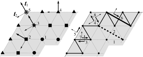
Figure 3: The 5 types of vertices (left) and the 8 types of vertices doublets (right) together with their local basis $\bm{t}_{1}$, $\bm{t}_{2}$ (the former being in thick arrows). Only the basis relative to the edges are indicated. For the doublet $(\alpha,\beta)$ of types 3,4,7 and 8, the begininng (resp. end) of the thick arrow corresponds to the first (resp. second) component $\alpha$ (resp. $\beta$) of the doublet.

We apply a similar procedure to assign a type to the oriented nearest and next-nearest neighbour vertex pairs, which we call vertex doublets. We distinguish the vertex doublets $(\alpha,\beta)$ from $(\beta,\alpha)$ since generally $\bm{A}^{\alpha\beta}\neq\bm{A}^{\beta\alpha}$. Two vertex doublets are assigned the same type if, and only if, their positions and orientations within the set of neighbour clusters in which they participate are indistinguishable. We thus determine eight types of vertex doublets, labeled from 1 to 8 (figure 3). The vertex doublets of type 1 are the bulk nearest-neighbour vertex doublets and those of type 2 are the bulk next-nearest neighbour vertex doublets. We also define types for the vertex pairs in the following way. When the two doublets associated with a given pair are of the same type, the pair is assigned that type (this holds for the types $1,2,5,6$) while the pairs corresponding to doublet types 3 and 7 are assigned the type 3 and those corresponding to doublet types 4 and 8 are assigned the type 4.

2.3.2 Symmetry allowed edge terms

In order to take into account the local symmetry up to the next-nearest neighbour distance, we consider the symmetries of the set of neighbour clusters in which the vertices or vertex doublets participate. Let us first examine the coefficients of the tensors $\bm{S}^{\alpha}$ for vertices of type 2 to 5 (edge vertices). Since each one possesses an axis of symmetry, we choose $\bm{t}_{1}$ along this axis and $\bm{t}_{2}\perp\bm{t}_{1}$ as indicated in figure 3. Then, as $\bm{S}^{\alpha}$ must be even in $\bm{t}_{2}$, we arrive at

$$\bm{S}^{\alpha}=s_{i}\,\bm{I_{2}}+\tilde{s}_{i}\,\bm{n}\otimes\bm{n}+\bar{s}_{i}\,\bm{\tau}^{\alpha}\otimes\bm{\tau}^{\alpha},\qquad(i={2},\ldots,{5})$$ (6)

where $\bm{\tau}^{\alpha}$ may either $\bm{t}_{1}$ or $\bm{t}_{2}$. For definiteness, we choose $\bm{\tau}^{\alpha}=\bm{t}_{2}$ for vertices of type 2 or 4 and $\bm{\tau}^{\alpha}=\bm{t}_{1}$ for vertices of type 3 or 5.

We now construct the tensor $\bm{A}^{\alpha\beta}$ for the vertex doublets of type 3 to 8 (edge types). The most general expression for $\bm{A}^{\alpha\beta}$ is given by an expression similar to (3):

$$\bm{A}^{\alpha\beta}\!\! = \!\!\frac{a_{\alpha\beta}}{2}\,\bm{I_{2}}+\frac{\tilde{a}_{\alpha\beta}}{2}\,\bm{n}\otimes\bm{n}+\frac{\bar{a}_{\alpha\beta}}{2}\,\bm{t}_{1}\otimes\bm{t}_{1}$$ (7)

$$+ \!\!\frac{\bar{\bar{a}}_{\alpha\beta}}{2}\,(\bm{t}_{1}\otimes\bm{t}_{2}+\bm{t}_{2}\otimes\bm{t}_{1})+\frac{a^{*}_{\alpha\beta}}{2}(\bm{t}_{1}\otimes\bm{t}_{2}-\bm{t}_{2}\otimes\bm{t}_{1}).$$

We choose $\bm{t}_{1}=\bm{t}^{\alpha\beta}$ and $\bm{t}_{2}$ as indicated in figure 3. The vertex doublets of types 4 and 8 have a mirror symmetry with respect to $\bm{t}_{1}$, hence $\bm{A}^{\alpha\beta}$ must be even in $\bm{t}_{2}$, which implies $\bar{\bar{a}}^{\alpha\beta}=a^{*\alpha\beta}=0$. Other relationships can be obtained by comparing the coefficients of $\bm{A}^{\alpha\beta}$ and those of $\bm{A}^{\beta\alpha}$. First, note that $(\bm{A}^{\alpha\beta})^{\mathrm{t}}=\bm{A}^{\beta\alpha}$ implies $a^{\alpha\beta}=a^{\beta\alpha}$, $\tilde{a}^{\alpha\beta}=\tilde{a}^{\beta\alpha}$, $\bar{a}^{\alpha\beta}=\bar{a}^{\beta\alpha}$, $\bar{\bar{a}}^{\alpha\beta}=-\bar{\bar{a}}^{\beta\alpha}$ and $a^{*\alpha\beta}=a^{*\beta\alpha}$. Then, since the vertex doublets of type 5 and 6 do not change type when exchanging $\alpha$ and $\beta$, their coefficients must satisfy $a^{\alpha\beta}=a^{\beta\alpha}$, $\tilde{a}^{\alpha\beta}=\tilde{a}^{\beta\alpha}$, $\bar{a}^{\alpha\beta}=\bar{a}^{\beta\alpha}$, $\bar{\bar{a}}^{\alpha\beta}=\bar{\bar{a}}^{\beta\alpha}$ and $a^{*\alpha\beta}=a^{*\beta\alpha}$. Therefore $\bar{\bar{a}}^{\alpha\beta}=0$ for types 5 and 6. Finally, we find

$$\bm{A}^{\alpha\beta}=\frac{a_{i}}{2}\,\bm{I_{2}}+\frac{\tilde{a}_{i}}{2}\,\bm{n}\otimes\bm{n}+\frac{\bar{a}_{i}}{2}\,\bm{t}^{\alpha\beta}\otimes\bm{t}^{\alpha\beta}+\frac{a_{i}^{*}}{2}\,\bm{\epsilon}^{\alpha\beta}+\frac{\bar{\bar{a}}_{i}}{2}\,\bm{\sigma}^{\alpha\beta},\quad(i=3,\ldots,8)$$ (8)

where $\bm{\epsilon}^{\alpha\beta}=\bm{t}_{1}\otimes\bm{t}_{2}-\bm{t}_{2}\otimes\bm{t}_{1}$, $\bm{\sigma}^{\alpha\beta}=\bm{t}_{1}\otimes\bm{t}_{2}+\bm{t}_{2}\otimes\bm{t}_{1}$ and $a_{4}^{*}=a_{8}^{*}=\bar{\bar{a}}_{4}=\bar{\bar{a}}_{8}=\bar{\bar{a}}_{5}=\bar{\bar{a}}_{6}=0$. In the following, we define $\bm{\epsilon}$ as the tensor that performs a counterclockwise $\frac{\pi}{2}$ rotation in the plane $\mathcal{P}$; depending on the relative orientations of $\bm{t}_{1}$ and $\bm{t}_{2}$, $\bm{\epsilon}^{\alpha\beta}$ is either equal to $\bm{\epsilon}$ or to $-\bm{\epsilon}$. Note that in general, we do find $\bm{A}^{\alpha\beta}\neq\bm{A}^{\beta\alpha}$, contrary to what is the case in the bulk.

2.3.3 Collecting edge terms

The total elastic energy can now be written as $F=F_{\text{bulk}}+F_{\text{edge}}$, with $F_{\text{bulk}}$ given by (5) and $F_{\text{edge}}$ obtained by collecting the edge terms defined above. We regroup the terms $\bm{u}^{\alpha}\cdot\bm{A}^{\alpha\beta}\cdot\bm{u}^{\beta}$ and $\bm{u}^{\beta}\cdot\bm{A}^{\beta\alpha}\cdot\bm{u}^{\alpha}$ in order to sum on the pairs and not on the doublets. We arrive then at

$$F_{\text{edge}}\!\! = \!\!\sum_{\alpha}\sum_{i={2}}^{5}\delta^{\alpha}_{i}\left[s_{i}(\bm{u}^{\alpha}_{\perp})^{2}+\tilde{s}_{i}(u^{\alpha}_{n})^{2}+\bar{s}_{i}(\bm{u}^{\alpha}_{\perp}\cdot\bm{\tau}^{\alpha})^{2}\right]$$ (9)

$$+ \!\!\sum_{<\alpha\beta>}\sum_{i={3}}^{6}\delta^{\alpha\beta}_{i}\left[a_{i}\,\bm{u}^{\alpha}_{\perp}\cdot\bm{u}^{\beta}_{\perp}+\tilde{a}_{i}\,u^{\alpha}_{n}u^{\beta}_{n}+\bar{a}_{i}(\bm{u}_{\perp}^{\alpha}\cdot\bm{t}^{\alpha\beta})(\bm{u}_{\perp}^{\beta}\cdot\bm{t}^{\alpha\beta})\right]$$

$$+ \!\!\!\!\!\mathrel{\hbox to0.0pt{\raise-0.5pt\hbox{\Large{\hskip 6.6pt{o}}}\hss}{\hbox{$\displaystyle\sum_{<\alpha\beta>}$}}}\!\left[\delta^{\alpha\beta}_{3}\,\eta^{\alpha\beta}\,\bar{\bar{a}}_{3}\,\bm{u}_{\perp}^{\alpha}\cdot\bm{\sigma}^{\alpha\beta}\cdot\bm{u}_{\perp}^{\beta}+\!\sum_{i={3,5,6}}\!\delta^{\alpha\beta}_{i}\,a_{i}^{*}\,\bm{u}_{\perp}^{\alpha}\cdot\bm{\epsilon}\cdot\bm{u}_{\perp}^{\beta}\right].$$

In this expression, $\delta^{\alpha}_{i}\in\{0,1\}$ and $\delta^{\alpha\beta}_{i}\in\{0,1\}$ are the indicatrix functions of the vertices of type $i$ and of the vertex pairs of type $i$, respectively (these types are defined in (2.3.1)) , and the symbol $\sum_{<\alpha\beta>}$ indicates the summation over all pairs $\{\alpha,\beta\}$ of vertices. The third line in (9) requires more explanations. We define a closed contour by grouping the vertex pairs of types 3 (see figure 3), another closed contour by grouping the vertex pairs of type 5, and three separate closed contours by grouping the vertex pairs of type 6. The symbol $\mathrel{\hbox to0.0pt{\raise-0.2pt\hbox{\large{\hskip 1.2pt{o}}}\hss}{\hbox{$\sum$}}}$ denotes the sums over all these contours followed counterclockwise. The symbol $\eta^{\alpha\beta}$ is equal to 1 or $-1$ according to whether the direction from $\alpha$ to $\beta$ goes outwards or inwards, respectively. Finally, in order to simplify the notation, we have renamed $\frac{1}{2}a_{4}+\frac{1}{2}a_{8}\to a_{4}$, $\frac{1}{2}\tilde{a}_{4}+\frac{1}{2}\tilde{a}_{8}\to\tilde{a}_{4}$, $\frac{1}{2}\bar{a}_{4}+\frac{1}{2}\bar{a}_{8}\to\bar{a}_{4}$, $\frac{1}{2}a_{3}^{*}+\frac{1}{2}a_{7}^{*}\to a_{3}^{*}$ and $\frac{1}{2}\bar{\bar{a}}_{3}^{*}-\frac{1}{2}\bar{\bar{a}}_{7}^{*}\to\bar{\bar{a}}_{3}^{*}$.

2.4 Rotational and translational invariance

Our task is now to ensure that the elastic energy remains unchanged if the lattice is translated or rotated as a whole. Although the general relationships are well-established (Born & Huang 1954), it is not an easy task to implement them in such a way as to put the elastic energy in a satisfactory form. Our strategy is to rearrange $F$ in order to put forward a number of terms that are obviously invariant, then to apply deliberately chosen translations or rotations in order to show that the remaining terms should vanish.

We first separate in $F$ ($=F_{\text{bulk}}+F_{\text{edge}}$) the contribution $F^{(n)}$ depending on the components $u^{\alpha}_{n}$ from the contribution $F^{(\perp)}$ depending on the components $\bm{u}^{\alpha}_{\perp}$. We thus have $F=F^{(n)}+F^{(\perp)}$ with

$$F^{(n)} = \sum_{\alpha}\sum_{i=1}^{5}\delta^{\alpha}_{i}\tilde{s}_{i}(u^{\alpha}_{n})^{2}+\sum_{<\alpha\beta>}\sum_{i=1}^{6}\delta^{\alpha\beta}_{i}\,\tilde{a}_{i}\,u^{\alpha}_{n}u^{\beta}_{n}\,,$$ (10)

$$F^{(\perp)} = \sum_{\alpha}\sum_{i=1}^{5}\delta^{\alpha}_{i}\left[s_{i}(\bm{u}^{\alpha}_{\perp})^{2}+\bar{s}_{i}(\bm{u}^{\alpha}_{\perp}\cdot\bm{\tau}^{\alpha})^{2}\right]$$ (11)

$$+ \!\!\sum_{<\alpha\beta>}\sum_{i=1}^{6}\delta^{\alpha\beta}_{i}\left[a_{i}\,\bm{u}^{\alpha}_{\perp}\cdot\bm{u}^{\beta}_{\perp}+\bar{a}_{i}(\bm{u}_{\perp}^{\alpha}\cdot\bm{t}^{\alpha\beta})(\bm{u}_{\perp}^{\beta}\cdot\bm{t}^{\alpha\beta})\right]$$

$$+ \!\!\!\!\!\mathrel{\hbox to0.0pt{\raise-0.5pt\hbox{\Large{\hskip 6.6pt{o}}}\hss}{\hbox{$\displaystyle\sum_{<\alpha\beta>}$}}}\!\left[\delta^{\alpha\beta}_{3}\,\eta^{\alpha\beta}\,\bar{\bar{a}}_{3}\,\bm{u}_{\perp}^{\alpha}\cdot\bm{\sigma}^{\alpha\beta}\cdot\bm{u}_{\perp}^{\beta}+\!\sum_{i={3,5,6}}\!\delta^{\alpha\beta}_{i}\,a_{i}^{*}\,\bm{u}_{\perp}^{\alpha}\cdot\bm{\epsilon}\cdot\bm{u}_{\perp}^{\beta}\right].$$

2.4.1 Translation invariance

Putting forward obviously translationally invariant terms in the form of differences, $F^{(n)}$ can be rewritten as

$$F^{(n)}=-\frac{1}{2}\sum_{<\alpha\beta>}\sum_{i={1}}^{6}\delta^{\alpha\beta}_{i}\,\tilde{a}_{i}\,(u_{n}^{\alpha}-u_{n}^{\beta})^{2}+\sum_{\alpha}\sum_{i={1}}^{5}\delta^{\alpha}_{i}\,C_{i}\,(u_{n}^{\alpha})^{2},$$ (12)

where the $C_{i}$ are linear combinations of the coefficients $\tilde{s}_{i}$ and $\tilde{a}_{j}$ (the coefficients in (12) still form an independent set). In the appendix, §.1, we show that the invariance of $F$ under any translation along $\bm{n}$ requires:

$$\forall i,\ C_{i}=0.$$ (13)

Similarly, $F^{(\perp)}$ can be written as obviously translationally invariant terms plus remainders:

$$F^{(\perp)} = -\frac{1}{2}\sum_{<\alpha\beta>}\sum_{i=1}^{6}\delta^{\alpha\beta}_{i}\,\left\{b_{i}\,(\bm{u}_{\perp}^{\alpha}-\bm{u}_{\perp}^{\beta})^{2}+\bar{b}_{i}\left[(\bm{u}_{\perp}^{\alpha}-\bm{u}_{\perp}^{\beta})\cdot\bm{t}^{\alpha\beta}\right]^{2}\right\}$$ (14)

$$- \!\!\!\sum_{<\alpha\beta\gamma>_{\text{IV}}}\!\!\!(1-\delta^{\alpha\beta\gamma}_{\text{IV},6})\frac{2}{\sqrt{3}}\,\bar{\bar{a}}_{3}\left[(\bm{u}^{\beta}_{\perp}-\bm{u}^{\alpha}_{\perp})\times\bm{t}^{\beta\alpha}-(\bm{u}^{\beta}_{\perp}-\bm{u}^{\gamma}_{\perp})\times\bm{t}^{\beta\gamma}\right]^{2}$$

$$+ \!\!\!\sum_{<\alpha\beta\gamma>_{\text{III}}}\,\sum_{i=3,5}\delta^{\alpha\beta\gamma}_{\text{III},i}\,b_{i}^{*}\,(\bm{u}_{\perp}^{\alpha}-\bm{u}_{\perp}^{\gamma})\cdot\bm{\epsilon}\cdot(\bm{u}_{\perp}^{\beta}-\bm{u}_{\perp}^{\gamma})$$

$$+ \!\!\!\sum_{<\alpha\beta\gamma>_{\text{V}}}\delta^{\alpha\beta\gamma}_{\text{V},6}\,b_{6}^{*}\,(\bm{u}_{\perp}^{\alpha}-\bm{u}_{\perp}^{\gamma})\cdot\bm{\epsilon}\cdot(\bm{u}_{\perp}^{\beta}-\bm{u}_{\perp}^{\gamma})$$

$$+ \!\sum_{\alpha}\sum_{i=2}^{5}\delta^{\alpha}_{i}\left[D_{i}\,(\bm{u}_{\perp}^{\alpha})^{2}+\bar{D}_{i}\,(\bm{u}_{\perp}^{\alpha}\cdot\bm{\tau}^{\alpha})^{2}\right].$$

Whereas the first line was clearly obtained by putting forward squares and discarding the remainders in the last line, the other lines deserve detailed explanations. Here and afterwards, the symbol $\sum_{<\alpha\beta\gamma>_{\text{Y}}}$ denotes the sum over all the triangular neighbour clusters of type Y, with $\alpha$, $\beta$ and $\gamma$ taken in counterclockwise order. For type IV, the vertex $\beta$ is supposed to be the central one, as in figure 2. The symbol $\delta^{\alpha\beta\gamma}_{\text{Y},i}$ is the indicatrix function of the neighbour clusters $\{\alpha,\beta,\gamma\}$ of type Y lying within the closed contour made by the vertex pairs of type $i$ ($i=3,5$ or 6). More precisely for $i=6$ it means to lie within at least one of the three closed contours made by the vertex pairs of type 6. In the following, we shall often encounter the translationally and rotationally invariant expression (as in the second line):

$$\left(\theta_{\alpha\beta\gamma}-\theta_{\alpha\beta\gamma}^{(0)}\right)^{2}=\left[(\bm{u}^{\beta}_{\perp}-\bm{u}^{\alpha}_{\perp})\times\bm{t}^{\beta\alpha}-(\bm{u}^{\beta}_{\perp}-\bm{u}^{\gamma}_{\perp})\times\bm{t}^{\beta\gamma}\right]^{2}+\mathcal{O}(u^{3})\,,$$ (15)

where $\theta_{\alpha\beta\gamma}$ and $\theta_{\alpha\beta\gamma}^{(0)}=\frac{\pi}{3}$ or $\frac{2\pi}{3}$ are the angles made by the vertices triplet $\{\alpha,\beta,\gamma\}$ with $\beta$ being the apex, after and before an elastic distortion of the lattice, respectively. In the appendix, § .2 (.2.1), we show how the terms involving $\bm{\sigma}^{\alpha\beta}$ in (11) were rewritten with the help of (15) and we give the expressions of the coefficients $b_{i}$ and $\bar{b}_{i}$ that were modified by this procedure. Finally, the lines involving $\bm{\epsilon}$ were obtained as detailed in the appendix, § .2 (.2.2). The coefficients $D_{i}$ and $\bar{D}_{i}$ are linear combinations of the coefficients $s_{i}$, $\bar{s_{i}}$, $a_{j}$, $\bar{a}_{j}$, $a_{j}^{*}$ and $\bar{\bar{a}}_{3}$ and the new coefficients in (14) still form an independent set. In the appendix, § .2 (.2.3), we show that the invariance of $F$ under in-plane translations requires:

$$\forall i,\ D_{i}=0\text{ and }\bar{D}_{i}=0.$$ (16)

Consequently, the total energy can be written in the following form, obviously invariant under any translation of the system:

$$F = -\sum_{<\alpha\beta>}\sum_{i=1}^{6}\frac{\delta^{\alpha\beta}_{i}}{2}\left\{\tilde{a}_{i}(u_{n}^{\alpha}-u_{n}^{\beta})^{2}+b_{i}(\bm{u}_{\perp}^{\alpha}-\bm{u}_{\perp}^{\beta})^{2}+\bar{b}_{i}\left[(\bm{u}_{\perp}^{\alpha}-\bm{u}_{\perp}^{\beta})\cdot\bm{t}^{\alpha\beta}\right]^{2}\right\}$$ (17)

$$- \!\!\!\sum_{<\alpha\beta\gamma>_{\text{IV}}}\!\!\!(1-\delta^{\alpha\beta\gamma}_{\text{IV},6})\frac{2}{\sqrt{3}}\,\bar{\bar{a}}_{3}\left[(\bm{u}^{\beta}_{\perp}-\bm{u}^{\alpha}_{\perp})\times\bm{t}^{\beta\alpha}-(\bm{u}^{\beta}_{\perp}-\bm{u}^{\gamma}_{\perp})\times\bm{t}^{\beta\gamma}\right]^{2}$$

$$+ \!\!\!\sum_{<\alpha\beta\gamma>_{\text{III}}}\,\sum_{i=3,5}\delta^{\alpha\beta\gamma}_{\text{III},i}\,b_{i}^{*}\,(\bm{u}_{\perp}^{\alpha}-\bm{u}_{\perp}^{\gamma})\cdot\bm{\epsilon}\cdot(\bm{u}_{\perp}^{\beta}-\bm{u}_{\perp}^{\gamma})$$

$$+ \!\!\!\sum_{<\alpha\beta\gamma>_{\text{V}}}\delta^{\alpha\beta\gamma}_{\text{V},6}\,b_{6}^{*}\,(\bm{u}_{\perp}^{\alpha}-\bm{u}_{\perp}^{\gamma})\cdot\bm{\epsilon}\cdot(\bm{u}_{\perp}^{\beta}-\bm{u}_{\perp}^{\gamma})$$

$$= F^{(n)}+F^{(\perp)},$$ (18)

where $F^{(n)}$ is the first term and $F^{(\perp)}$ is the sum of all the other terms.

2.4.2 Rotation invariance

Putting forward rotationally invariant terms, $F^{(n)}$, as obtained from (17), can be rewritten as

$$F^{(n)} = \frac{1}{2}k_{n1}\!\!\!\!\!\!\!\sum_{<\alpha\beta\gamma\delta>_{\text{VI}}}\!\!\!\!\!\theta^{2}_{\alpha\beta\gamma\delta}+\frac{1}{2}k_{n2}\!\!\!\!\!\!\sum_{<\alpha\beta\gamma\delta>_{\text{VII}}}\!\!\!\!\!\!\theta^{2}_{\alpha\beta\gamma\delta}$$ (19)

$$+ \!\!\!\sum_{<\alpha\beta>\,}\sum_{\,i=2,4,5,6}\delta_{\alpha\beta}^{i}\,E_{i}\left(u_{n}^{\alpha}-u_{n}^{\beta}\right)^{2}+\mathcal{O}(u^{3})\,.$$

The symbol $\sum_{<\alpha\beta\gamma\delta>_{\text{Y}}}$ denotes the sum over all the neighbour clusters of type Y=VI or VII with the vertices placed as shown in figure 2. The angle $\theta_{\alpha\beta\gamma\delta}$ denotes the wedge angle between the planes defined by the vertices $(\alpha,\beta,\gamma)$ and the vertices $(\alpha,\beta,\delta)$. In the appendix, § .3 (.3.1), we show how the wedge angles are related to the normal displacements $u_{n}^{\alpha}$. The coefficients $E_{i}$ are linear combinations of $\tilde{a}_{i}$, $\tilde{a}_{1}$ and $\tilde{a}_{3}$, and the new coefficients still form an independent set. We show in the appendix, § .3 (.3.2), that the invariance of $F$ with respect to out-of-plane rotations requires:

$$\forall i,\ E_{i}=0.$$ (20)

Finally, we put forward in $F^{(\perp)}$ seven rotationally invariant terms, obtained by considering various energy terms associated with deviations of lengths or angles with respect to their equilibrium values:

$$F^{(\perp)}\!\! = \!\!\frac{1}{2}\sum_{<\alpha\beta>}\sum_{i=1}^{6}\delta^{\alpha\beta}_{i}\,k_{i}\!\left(\ell_{\alpha\beta}-\ell\right)^{2}+\frac{1}{2}k_{\frac{\pi}{3}}\!\!\!\!\sum_{<\alpha\beta\gamma>_{\text{III}}}\!\!\!\!\delta^{\alpha\beta\gamma}_{\text{III},3}\left[\left(\theta_{\alpha\beta\gamma}-\frac{\pi}{3}\right)^{2}+\text{c.\,p.}\right]$$ (21)

$$+ \!\!\frac{1}{2}k^{\prime}_{\frac{\pi}{3}}\!\!\!\!\sum_{<\alpha\beta\gamma>_{\text{V}}}\!\!\!\!\delta^{\alpha\beta\gamma}_{\text{V},6}\left[\left(\theta_{\alpha\beta\gamma}-\frac{\pi}{3}\right)^{2}+\text{c.\,p.}\right]$$

$$+ \!\!\frac{1}{2}k^{\prime\prime}_{\frac{\pi}{3}}\!\!\!\!\sum_{<\alpha\beta\gamma>_{\text{III}}}\!\!\!\!(\delta^{\alpha\beta\gamma}_{\text{III},5}-\delta^{\alpha\beta\gamma}_{\text{III},3})\left[\left(\theta_{\alpha\beta\gamma}-\frac{\pi}{3}\right)^{2}+\text{c.\,p.}\right]$$

$$+ \!\!\frac{1}{2}k_{\frac{2\pi}{3}}\!\!\!\!\sum_{<\alpha\beta\gamma>_{\text{IV}}}\!\!\!\!\delta^{\alpha\beta\gamma}_{\text{IV},6}\left(\theta_{\alpha\beta\gamma}-\frac{2\pi}{3}\right)^{2}+\frac{1}{2}k^{\prime}_{\frac{2\pi}{3}}\!\!\!\!\sum_{<\alpha\beta\gamma>_{\text{IV}}}\!\!\!\!\left(1-\delta^{\alpha\beta\gamma}_{\text{IV},6}\right)\left(\theta_{\alpha\beta\gamma}-\frac{2\pi}{3}\right)^{2}$$

$$+ \!\!\frac{1}{2}k_{\frac{\pi}{6}}\!\!\!\!\sum_{<\alpha\beta\gamma>_{\text{IV}}}\!\!\!\!\left(1-\delta_{\alpha\beta\gamma}^{\text{IV},6}\right)\left[\left(\theta_{\beta\gamma\alpha}-\frac{\pi}{6}\right)^{2}\!+\left(\theta_{\beta\alpha\gamma}-\frac{\pi}{6}\right)^{2}\right]$$

$$+ \!\!\!\!\!\!\sum_{<\alpha\beta\gamma>_{\text{III}}}\sum_{\,i=3,5}\delta_{\text{III},i}^{\alpha\beta\gamma}\,G_{i}^{*}(\bm{u}_{\perp}^{\alpha}-\bm{u_{\perp}}^{\gamma})\cdot\bm{\epsilon}\cdot(\bm{u}_{\perp}^{\beta}-\bm{u}_{\perp}^{\gamma}),$$

$$+ \!\!G_{6}^{*}\!\!\!\!\sum_{<\alpha\beta\gamma>_{\text{V}}}\!\!\!\!\delta_{\text{V},6}^{\alpha\beta\gamma}\,(\bm{u}_{\perp}^{\alpha}-\bm{u_{\perp}}^{\gamma})\cdot\bm{\epsilon}\cdot(\bm{u}_{\perp}^{\beta}-\bm{u}_{\perp}^{\gamma})+G\!\!\sum_{<\alpha\beta>}\delta^{\alpha\beta}_{3}(\bm{u}^{\alpha}_{\perp}-\bm{u}^{\beta}_{\perp})^{2}\,.$$

The abbreviation c. p. stands for ‘circular permutations’ of $\{\alpha,\beta,\gamma\}$ and $\ell_{\alpha\beta}$ is the distance between the vertices $\alpha$ and $\beta$. The detail of how (21) and (17) are related is given in the appendix, § .4 (.4.1). The coefficient $G$ is a linear combination of $b_{3}$ and the other $b_{i}$’s and the coefficients $G_{i}^{*}$ are linear combinations of the corresponding $b_{i}^{*}$ and the $b_{j}$’s ($j\neq 3$). The new coefficients still form an independent set. In the appendix, § .4 (.4.2), we show that the invariance of $F$ with respect to in-plane rotations implies

$$G=0\quad\text{and}\quad\forall i,\ G^{*}_{i}=0.$$ (22)

2.5 Final expression of the bulk terms

From the preceeding section, it follows that the most general elastic energy $F$ of an hexagonal triangular lattice, invariant with respect to translation and rotations, is given by the sum of (19) and (21), with all the $E_{i}$’s, $G_{i}^{*}$’s and G equal to zero.

Putting forward the bulk terms, and expressing them in terms of the displacements instead of angles and lengths (using (15) and the the formulas of the appendix, § .3 (.3.1) and § .4 (.4.1)), we finally obtain

$$F\!\! =\!\! \frac{1}{2}k_{n1}\!\!\!\!\!\!\sum_{<\alpha\beta\gamma\delta>_{\text{VI}}}\frac{4}{3\ell^{2}}\left(u_{n}^{\delta}+u_{n}^{\gamma}-u_{n}^{\alpha}-u_{n}^{\beta}\right)^{2}$$ (23)

$$+ \!\!\frac{1}{2}k_{n2}\!\!\!\!\!\!\sum_{<\alpha\beta\gamma\delta>_{\text{VII}}}\frac{4}{3\ell^{2}}\left(3u_{n}^{\alpha}-u_{n}^{\beta}-u_{n}^{\gamma}-u_{n}^{\delta}\right)^{2}$$

$$+ \!\!\frac{1}{2}k\!\!\sum_{<\alpha\beta>}\frac{\delta^{\alpha\beta}_{1}}{\ell^{2}}\,\left[(\bm{u}^{\alpha}-\bm{u}^{\beta})\cdot\bm{t}^{\alpha\beta}\right]^{2}+\frac{1}{2}k^{\prime}\!\!\sum_{<\alpha\beta>}\frac{\delta^{\alpha\beta}_{2}}{\ell^{2}}\,\left[(\bm{u}^{\alpha}-\bm{u}^{\beta})\cdot\bm{t}^{\alpha\beta}\right]^{2}$$

$$+ \!\!\frac{1}{2}k_{\frac{\pi}{3}}\!\!\!\!\!\sum_{<\alpha\beta\gamma>_{\text{III}}}\!\!\!\frac{1}{\ell^{2}}\,\delta^{\alpha\beta\gamma}_{\text{III},3}\left\{\left[(\bm{u}^{\alpha}_{\perp}-\bm{u}^{\beta}_{\perp})\times\bm{t}^{\alpha\beta}-(\bm{u}^{\alpha}_{\perp}-\bm{u}^{\gamma}_{\perp})\times\bm{t}^{\alpha\gamma}\right]^{2}+\text{c.\,p.}\right\}\hskip 19.91684pt$$

$$+ \!\!\frac{1}{2}k_{\frac{\pi}{3}}^{\prime}\!\!\!\!\!\sum_{<\alpha\beta\gamma>_{\text{V}}}\!\!\frac{1}{3\ell^{2}}\,\delta^{\alpha\beta\gamma}_{\text{V},6}\left\{\left[(\bm{u}^{\alpha}_{\perp}-\bm{u}^{\beta}_{\perp})\times\bm{t}^{\alpha\beta}-(\bm{u}^{\alpha}_{\perp}-\bm{u}^{\gamma}_{\perp})\times\bm{t}^{\alpha\gamma}\right]^{2}+\text{c.\,p.}\right\}$$

$$+ \!\!\frac{1}{2}k_{\frac{2\pi}{3}}\!\!\!\!\!\sum_{<\beta\alpha\gamma>_{\text{IV}}}\!\!\delta^{\beta\alpha\gamma}_{\text{IV},6}\,\frac{1}{\ell^{2}}\left[(\bm{u}^{\alpha}_{\perp}-\bm{u}^{\beta}_{\perp})\times\bm{t}^{\alpha\beta}-(\bm{u}^{\alpha}_{\perp}-\bm{u}^{\gamma}_{\perp})\times\bm{t}^{\alpha\gamma}\right]^{2}+\ldots$$

where $k=k_{1}$ and $k^{\prime}=k_{2}$ and the ellipsis represent terms involving only edge vertex pairs.

3 Analysis

3.1 Comments on the energy form (23)

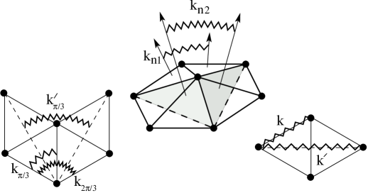
Figure 4: Interpretation of the elastic terms in (23) in terms of linear and angular springs: The top drawing is in perspective while the others are in projection. The arrows are normal to the facets. The springs with elastic modulus $k$ (resp. $k^{\prime}$) have an equilibrium length $\ell$ (resp. $\ell\sqrt{3})$. The angular springs with moduli $k_{n1}$ and $k_{n2}$ (elastic wedges) have zero equilibrium angles; the angular springs with moduli $k_{\psi}$ or $k^{\prime}_{\psi}$ have equilibrium angles $\psi$.

As shown in figure 4, each term of (23) can be given a simple interpretation in terms of linear or angular springs. The terms with coefficients $k_{ni}$, corresponding to elastic wedges, tend to keep the lattice flat and yield a form of curvature energy. The terms with coefficients $k$ and $k^{\prime}$ represent elastic bonds acting between nearest and next-nearest neighbours, respectively. The terms with moduli $k_{\frac{\pi}{3}}$, $k^{\prime}_{\frac{\pi}{3}}$ and $k_{\frac{2\pi}{3}}$ are angular springs acting at the bond joints.

The decomposition (23) is in many respects non-unique. For instance, the term with coefficient $k_{n2}$ could be omitted if we are only interested in the bulk terms, for it has the same decomposition on the bulk vertex pairs as the term with coefficient $k_{n1}$; this can be easily checked by comparing the coefficients of $\delta^{\alpha\beta}_{1}$ and $\delta^{\alpha\beta}_{2}$ in the equations of the appendix, § .3 (.3.1). Note, however, that the expressions of these two energies in terms of clusters of four vertices differ, as we can see in the two first terms of (23). As another example, we could have included in (23) energy terms associated with the $\frac{\pi}{6}$ angles in the bulk neighbour clusters of type IV; this would bring nothing new, since they can be written as a linear combination of other terms that are already present:

$$\!\!\sum_{<\beta\alpha\gamma>_{\text{IV}}}\!\!\!\!\delta^{\beta\alpha\gamma}_{\text{IV},6}\left[\left(\theta_{\alpha\beta\gamma}-\frac{\pi}{6}\right)^{2}+\left(\theta_{\beta\gamma\alpha}-\frac{\pi}{6}\right)^{2}\right]+\mathcal{O}(u^{3})$$

$$\!\!=\frac{1}{6}\!\!\sum_{<\alpha\beta\gamma>_{\text{V}}}\!\!\!\!\delta^{\alpha\beta\gamma}_{\text{V},6}\left[\left(\theta_{\beta\alpha\gamma}-\frac{\pi}{3}\right)^{2}+\text{c.\,p.}\right]+\frac{1}{2}\!\!\sum_{<\beta\alpha\gamma>_{\text{IV}}}\!\!\!\!\delta^{\beta\alpha\gamma}_{\text{IV},6}\left(\theta_{\beta\alpha\gamma}-\frac{2\pi}{3}\right)^{2}\,.\qquad$$ (24)

Nonetheless, although the form of (23) depends on the choices we made during the various transformations on the energy, our procedure guarantees that it does correspond to the most general elastic energy of a triangular lattice up to next-nearest neighbour interactions.

3.2 Compact expression of the elastic energy

With the help of the formulas given in the appendix, § .3 (.3.1) and § .4 (.4.1), the energy (23) can be rewritten in a more compact form, in terms of the normal, transversal and longitudinal components of the relative displacements between nearest and next-nearest neighbours :

$$F\!\! = \!\!\frac{1}{2}\!\!\sum_{<\alpha\beta>_{\text{I}}}\!\!\left\{K_{n}(u_{n}^{\alpha}-u_{n}^{\beta})^{2}+K_{t}\left[(\bm{u}_{\perp}^{\alpha}-\bm{u}_{\perp}^{\beta})\cdot\bm{t}_{\perp}^{\alpha\beta}\right]^{2}\!\!\!+K_{\ell}\left[(\bm{u}_{\perp}^{\alpha}-\bm{u}_{\perp}^{\beta})\cdot\bm{t}^{\alpha\beta}\right]^{2}\right\}$$ (25)

$$+ \!\!\frac{1}{2}\!\!\sum_{<\alpha\beta>_{\text{II}}}\!\!\!\left\{-\frac{K_{n}}{3}(u_{n}^{\alpha}-u_{n}^{\beta})^{2}\!+K_{t}^{\prime}\left[(\bm{u}_{\perp}^{\alpha}-\bm{u}_{\perp}^{\beta})\cdot\bm{t}^{\alpha\beta}_{\perp}\right]^{2}\!\!+K_{\ell}^{\prime}\left[(\bm{u}_{\perp}^{\alpha}-\bm{u}_{\perp}^{\beta})\cdot\bm{t}^{\alpha\beta}\right]^{2}\right\}$$

$$+ \!\!\text{edge terms},$$

where $\bm{t}_{\perp}^{\alpha\beta}\equiv\bm{n}\times\bm{t}^{\alpha\beta}$, and the symbols $\sum_{<\alpha\beta>_{\text{I}}}$ and $\sum_{<\alpha\beta>_{\text{II}}}$ indicate the sum over all the neighbour clusters of type I and II, i.e. over the pairs of nearest and next-nearest vertices, respectively. The normal coefficient, which corresponds to curvature energy, is given by $K_{n}=\ell^{-2}(4k_{n1}+12k_{n2})$. The transverse coefficients $K_{t}$ and $K_{t}^{\prime}$ are given by $K_{t}=\ell^{-2}(\frac{3}{2}k_{\pi/3}+6k_{2\pi/3})$ and $K_{t}^{\prime}=\ell^{-2}(\frac{1}{2}k^{\prime}_{\pi/3}-\frac{3}{2}k_{2\pi/3})$, and the longitudinal coefficients $K_{\ell}$ and $K_{\ell}^{\prime}$ are given by $K_{\ell}=\ell^{-2}(k+\frac{3}{2}k_{\pi/3})$ and $K_{\ell}^{\prime}=\ell^{-2}(k^{\prime}+\frac{1}{2}k_{\pi/3}^{\prime}+\frac{1}{2}k_{2\pi/3}).$ These new coefficients are independent linear combinations of the former. Moreover, the five functions of $\{\bm{u}^{\alpha}\}$ (proportional to the coefficients $K_{n}$, $K_{t}$, $K_{\ell}$, $K^{\prime}_{t}$ and $K^{\prime}_{\ell}$), appearing in the form (25), can be shown to be linearly independent in their functional space. Therefore, the seven (or more) rigidities which one could associate with the mechanical elements drawn in figure 4 reduce to only five independent elastic constants.

A number of comments follow. The angular coefficients of (23), i.e. $k_{\pi/3}$, $k_{\pi/3}^{\prime}$ and $k_{2\pi/3}$, are present both in the tranverse and the longitudinal coefficients: this is because in a triangular lattice one cannot change the angles between bonds without changing the distances between the vertices. Conversely, the coefficients $k$ and $k^{\prime}$ appear only in the longitudinal coefficients. Also, as explained above, the two coefficients $k_{n1}$ and $k_{n2}$ collapse into a unique normal coefficient $K_{n}$. Most importantly, note that the non-central term with coefficients $K_{t}$, which was understood from Keating (1966) to violate rotational invariance, is actually allowed (even if we restrain the model to nearest neighbour interaction only). We shall comment on this in §4.

Finally, although (25) is expressed as a sum of squared terms, the stability issue is not trivial, since these terms are not independent. For instance, the stability of the undistorted lattice does not require all the five coefficients of (25) to be positive. For example, if all the coefficients in (23) are positive, which is obviously a sufficient condition for stability, and if $k_{\frac{2\pi}{3}}>\frac{1}{3}k^{\prime}_{\pi/3}$, we may have $K^{\prime}_{t}<0$. Further comments on the statibility issue will be given in §4.

3.3 Link with the continuous theory

In a continuous description, the displacement of the point $\bm{r}$ on the plane $\mathcal{P}$ is described by a three-dimensional continuous function $\bm{u}(\bm{r})$. In order to link the discrete description to the continuous one, we assume that the displacements $\bm{u}^{\alpha}$ vary very slowly at the scale of the lattice spacing $\ell$ and we identify $\bm{u}^{\alpha}$ and $\bm{u}(\bm{r}^{\alpha})$. Hence, we transform (25) with the help of the Taylor expansion:

$$\bm{u}^{\beta}-\bm{u}^{\alpha}=\xi\,\bm{t}^{\alpha\beta}\cdot\bm{\nabla}\bm{u}\left(\bm{r}^{\alpha}\right)+\mathcal{O}(\xi^{2})\,,$$ (26)

where $\bm{r}^{\beta}-\bm{r}^{\alpha}=\xi\,\bm{t}^{\alpha\beta}$, with $\xi=\ell$ for nearest neighbour vertices and $\xi=\ell\sqrt{3}$ for next-nearest neighbour vertices, and $\sum_{\alpha}\to 2\ell^{-2}/\sqrt{3}\int\!\rd^{2}r$. We take an orthonormal coordinate system $(x,y,z)$, with the $z$ axis parallel to $\bm{n}$ and the $x$ axis along one of the three nearest-neighbour directions of the undistorted lattice. Then, for the in-plane part $F^{(\perp)}$ of (25), we obtain $F^{(\perp)}=\int\!\rd^{2}r\,f^{(\perp)}$, with

$$f^{(\perp)}\!\!\! = \!\!\!\bar{K}_{\ell}\left[3\left(u^{x}_{,x}\right)^{2}+3\left(u^{y}_{,y}\right)^{2}+\left(u^{x}_{,y}\right)^{2}+\left(u^{y}_{,x}\right)^{2}+2\,u^{x}_{,x}\,u^{y}_{,y}+2\,u^{x}_{,y}\,u^{y}_{,x}\right]$$ (27)

$$+ \!\!\!\bar{K}_{t}\left[\left(u^{x}_{,x}\right)^{2}+\left(u^{y}_{,y}\right)^{2}+3\left(u^{x}_{,y}\right)^{2}+3\left(u^{y}_{,x}\right)^{2}-2\,u^{x}_{,x}\,u^{y}_{,y}-2\,u^{x}_{,y}\,u^{y}_{,x}\right],\quad$$

in which $\bar{K}_{\ell}=\frac{1}{8}\sqrt{3}(K_{\ell}+3K^{\prime}_{\ell})$ and $\bar{K}_{t}=\frac{1}{8}\sqrt{3}(K_{t}+3K^{\prime}_{t})$ and $u_{,j}^{i}$ is the derivative of the $i$th component of $\bm{u}$ with respect to the $j$th component of $\bm{r}$ (note that $i\in\{x,y,z\}$ whereas $j\in\{x,y\}$). Using integrations by parts, we can rewrite the energy density in the standard, isotropic, form $f^{(\perp)}=\frac{1}{2}\lambda\,e_{ii}\,e_{jj}+\mu\,e_{ij}\,e_{ij}$, with $e_{ij}=\frac{1}{2}(u^{i}_{,j}+u^{j}_{,i})$. The Lamé coefficients are given by

$$\lambda\!\! = \!\!\frac{\sqrt{3}}{4}\left[K_{\ell}+3K_{\ell}^{\prime}-5\left(K_{t}+3K_{t}^{\prime}\right)\right],$$ (28)

$$\mu\!\! = \!\!\frac{\sqrt{3}}{4}\left[K_{\ell}+3K_{\ell}^{\prime}+3\left(K_{t}+3K_{t}^{\prime}\right)\right].$$ (29)

In terms of the spring constants of (23), this gives $\lambda=\frac{3}{2}\sqrt{3}\,\ell^{-2}(\frac{1}{6}k+\frac{1}{2}k^{\prime}-k_{\pi/3}-k^{\prime}_{\pi/3}-k_{2\pi/3})$ and $\mu=\frac{3}{2}\sqrt{3}\,\ell^{-2}(\frac{1}{6}k+\frac{1}{2}k^{\prime}+k_{\pi/3}+k^{\prime}_{\pi/3}+k_{2\pi/3})$. For a system composed only of springs between nearest neighbours, we recover the classical relation $\lambda=\mu=\frac{1}{4}\sqrt{3}\,k/\ell^{2}$ (Kantor et al. 1987). As expected, the area compressibility modulus $K_{A}=\lambda+\mu$ depends only on the spring constants and not on the angular constants: $\lambda+\mu=\frac{1}{2}\sqrt{3}\,(K_{\ell}+3K_{\ell}^{\prime}-K_{t}-3K_{t}^{\prime})=\frac{1}{2}\sqrt{3}\,\ell^{-2}(k+3k^{\prime})$.

For the normal part $F^{(n)}$ of the energy, it is necessary to add the second order terms $\frac{1}{2}\xi^{2}\,\bm{t}^{\alpha\beta}\cdot\bm{\nabla}\bm{\nabla}\bm{u}\cdot\bm{t}^{\alpha\beta}$ in the Taylor expansion because the first order vanishes. With $F^{(n)}=\int\!\rd^{2}r\,f^{(n)}$, we obtain the isotropic energy density

$$f^{(n)}=\frac{1}{2}\kappa\left(u^{z}_{,xx}+u^{z}_{,yy}\right)^{2},$$ (30)

with the bending constant $\kappa=\frac{1}{8}\ell^{2}\sqrt{3}\,K_{n}=\frac{\sqrt{3}}{2}(k_{n1}+3k_{n2})$. One recognises the bending energy associated with the curvature $H=\frac{1}{2}(u^{z}_{,xx}+u^{z}_{,yy})+\mathcal{O}(u^{3})$ of the surface $z=u^{z}(\bm{r})$.

4 Summary and discussion

In this paper, we have determined the most general form for the elastic energy of a triangular lattice when both first and second neighbour couplings are taken into account. We have found that, among the six coefficients originating from the decomposition of the energy in terms of the normal, transversal and longitudinal components of the relative displacements between nearest and next-nearest neighbours, only five are independent (equation (3.2)). Consequently, only five combinations of the elastic parameters given for instance in figure 4 are measurable. We have also found that only three coefficients survive in the large scale limit, the Lamé coefficients and the bending modulus; therefore our discrete description introduces two new elastic coefficients. From the following well-known stability criteria: $\kappa>0$, $\mu>0$ and $\lambda+\mu>0$, it is possible to deduce some necessary stability conditions: $K_{n}>0$, $K_{\ell}+3K_{\ell}^{\prime}>0$ and $K_{t}+3K_{t}^{\prime}>-\frac{1}{3}K_{\ell}-K_{\ell}^{\prime}$. A complete stability analysis can be performed by Fourier transform. However, the additional stability conditions on the coefficients being rather intricate, we shall not describe them here.

One of the main issue in the paper was the necessity to take into account the boundary elastic energy in order to correctly impose rotational invariance. This is well exemplified by the following energy term, which represents the sum of the energies of the angular springs between nearest bonds:

$$\sum_{i}\left(\theta_{i}-\frac{\pi}{3}\right)^{2}\!\!\! = \!\!\!\sum_{\alpha-\beta}^{(B)}\frac{3}{2}\left(\bm{u}^{\alpha}_{\perp}-\bm{u}^{\beta}_{\perp}\right)^{2}$$ (31)

$$+ \!\!\!\sum_{\alpha-\beta}^{(\partial B)}\frac{3}{4}\left(\bm{u}^{\alpha}_{\perp}-\bm{u}^{\beta}_{\perp}\right)^{2}+\mathrel{\hbox to0.0pt{\raise-0.5pt\hbox{\Large{\hskip 4.6pt{o}}}\hss}{\hbox{$\displaystyle\sum_{\alpha\to\beta}^{(\partial B)}$}}}\frac{3\sqrt{3}}{2}\,\bm{u}_{\perp}^{\alpha}\cdot\bm{\epsilon}\cdot\left(\bm{u}^{\beta}_{\perp}-\bm{u}^{\alpha}_{\perp}\right),$$

where $i$ runs over all the pairs of adjacent bonds, making an angle $\theta_{i}$, and $\alpha\!-\!\beta$ runs over the interior bonds when $(B)$ is indicated, or over the boundary bonds when $(\partial B)$ is indicated. In the last sum, the bonds ($\alpha\!\!\to\!\!\beta$) must be taken counterclockwise. Indeed, the left-hand side is manifestly rotationally invariant and, under an infinitesimal in-plane rotation $\bm{u}^{\alpha}_{\perp}=\omega\,\bm{n}\times\bm{r}^{\alpha}$, the last term of the right-hand side (r.-h. s.), which is a boundary term, can be shown to yield an extensive contribution $-2\omega^{2}\,A$, where $A$ is the area of the lattice, just as the first term of the r.-h. s, which is a bulk term. It follows that: i) this first term is not rotationally invariant by itself, ii) that boundary terms are therefore necessary to correctly ensure rotational invariance, and that, as announced, iii) the term with coefficient $K_{t}$ is indeed allowed, even if we restrain the model to nearest neighbour interaction only.

In conclusion, the method developed in this paper—which consists in defining neighbour clusters based on the interaction range, in considering explicitely the edges of the lattice, in considering the local symmetries defined in terms of cluster environment to distinguish the various edge terms, etc.—provides a safe basis to further implement rotational invariance. This method could be applied to a large variety of lattices and to higher dimensions. Translational and rotational invariances

This appendix contains the detail of the calculations made to impose translational and rotational invariances to the elastic energy.

.1 Translation parallel to $\bm{n}$

Here we demonstrate (13), on the basis of (12). Substituting $\bm{u}^{\alpha}=\xi\,\bm{n}$ in equation (12) yields $F^{(n)}/\xi^{2}=\sum_{i=1}^{5}C_{i}V_{i}$, where the coefficients $V_{i}$ are defined in the table of figure 5. Hence, with $\xi=1$,

$$F^{(n)}=3N^{2}C_{1}+3N\left(-9C_{1}+6C_{2}+6C_{4}\right)+7C_{1}-12C_{2}+6C_{3}-6C_{4}+6C_{5}\,\,\,$$ (32)

Setting $F^{(n)}=0$ for all $N$ implies $0=C_{1}=C_{2}+C_{4}=C_{3}+C_{4}+C_{5}$. Next, imposing the same translation but from a distorted state, defined by $\bm{u}^{\alpha}=\bm{0}$ except for one vertex $\alpha_{0}$ of type 4 (resp. 5) for which $\bm{u}^{\alpha_{0}}=\xi_{0}\bm{n}$, it is straightforward to show that the invariance of $F$ requires $C_{4}=0$ (resp. $C_{5}=0$). Consequently, all the coefficients $C_{i}$ must vanish.

Type	Vertex	Pairs of vertices
1	$V_{1}=3N^{2}-9N+7$	$P_{1}=9N^{2}-15N+6$
2	$V_{2}=6N-12$	$P_{2}=9N^{2}-15N+6$
3	$V_{3}=6$	$P_{3}=12N-12$
4	$V_{4}=6N-6$	$P_{4}=6$
5	$V_{5}=6$	$P_{5}=6N$
6		$P_{6}=12N-6$

Figure 5: Number of vertices, $V_{i}$, and of pair of vertices, $P_{i}$, as a function of their type (see figure 3) for a regular hexagon of edge length $N\ell$.

.2 Translation parallel to $\mathcal{P}$

Here we display in (.2.1) and (.2.2) some details of the calculations made to go from (11) to (14) and we demonstrate in (.2.3) the equation (16) on the basis of equation (14).

.2.1 Treatment of the terms involving $\bm{\sigma}^{\alpha\beta}$.

In the process to obtain equation (14), the terms involving $\bm{\sigma}^{\alpha\beta}$ in (11) have been eliminated using the following identity:

$$\!\!\!\!\!\!\sum_{<\alpha\beta\gamma>_{\text{IV}}}\!\!\!\!\!\left(1-\delta^{\alpha\beta\gamma}_{\text{IV},6}\right)\frac{2}{\sqrt{3}}\left[(\bm{u}^{\beta}_{\perp}-\bm{u}^{\alpha}_{\perp})\times\bm{t}^{\beta\alpha}-(\bm{u}^{\beta}_{\perp}-\bm{u}^{\gamma}_{\perp})\times\bm{t}^{\beta\gamma}\right]^{2}$$

$$\!\!\!\!\!=\!\!\!\!\sum_{<\alpha\beta\gamma>_{\text{IV}}}\!\!\!\!\!\left(1-\delta^{\alpha\beta\gamma}_{\text{IV},6}\right)\frac{8}{3\sqrt{3}}\left[(\bm{u}^{\alpha}_{\perp}-\bm{u}^{\beta}_{\perp})\!\cdot\!\left(\bm{t}^{\beta\gamma}\!+\!\frac{\bm{t}^{\beta\alpha}}{2}\right)+(\bm{u}^{\gamma}_{\perp}-\bm{u}^{\beta}_{\perp})\!\cdot\!\left(\bm{t}^{\beta\alpha}\!+\!\frac{\bm{t}^{\beta\gamma}}{2}\right)\right]^{2}\!\!$$

$$\!\!\!\!\!=\sum_{\alpha}\frac{\sqrt{3}}{2}\,\left(\delta^{\alpha}_{2}-\delta^{\alpha}_{3}+\delta^{\alpha}_{4}\right)\left[\left(\bm{u}_{\perp}^{\alpha}\right)^{2}-2\left(\bm{u}^{\alpha}\cdot\bm{\tau}^{\alpha}\right)^{2}\right]$$

$$\!\!\!\!\!-\mathrel{\hbox to0.0pt{\raise-0.5pt\hbox{\Large{\hskip 6.6pt{o}}}\hss}{\hbox{$\displaystyle\sum_{<\alpha\beta>}$}}}\left[\delta^{\alpha\beta}_{3}\,\eta^{\alpha\beta}\,\bm{u}^{\alpha}\cdot\bm{\sigma}^{\alpha\beta}\cdot\bm{u}^{\beta}+\left(\delta^{\alpha\beta}_{3}+2\delta^{\alpha\beta}_{5}-\delta^{\alpha\beta}_{6}\right)\left(\bm{u}^{\alpha}\cdot\bm{\epsilon}\cdot\bm{u}^{\beta}\right)\right]$$

$$\!\!\!\!\!+\sum_{<\alpha\beta>}\!\!\!\sqrt{3}\,\bigg{\{}\!\!\left(\delta^{\alpha\beta}_{3}+2\delta^{\alpha\beta}_{5}-\frac{1}{2}\delta^{\alpha\beta}_{6}\right)\left(\bm{u}_{\perp}^{\alpha}-\bm{u}_{\perp}^{\beta}\right)^{2}$$

$$\qquad\qquad\left.+\left(-\delta^{\alpha\beta}_{3}-2\delta^{\alpha\beta}_{5}+\frac{2}{3}\delta^{\alpha\beta}_{6}\right)\left[\left(\bm{u}^{\alpha}-\bm{u}^{\beta}\right)\cdot\bm{t}^{\alpha\beta}\right]^{2}\right\}.$$ (33)

The coefficients $b_{i}$ and $\bar{b}_{i}$ in equation (14) are then given by $b_{1}=a_{1}$, $\bar{b}_{1}=\bar{a}_{1}$, $b_{2}=a_{2}$, $\bar{b}_{2}=\bar{a}_{2}$, $b_{3}=a_{3}-2\sqrt{3}\,\bar{\bar{a}}_{3}$, $\bar{b}_{3}=\bar{a}_{3}+2\sqrt{3}\,\bar{\bar{a}}_{3}$, $b_{4}=a_{4}$, $\bar{b}_{4}=\bar{a}_{4}$, $b_{5}=a_{5}-4\sqrt{3}\,\bar{\bar{a}}_{3}$, $\bar{b}_{5}=\bar{a}_{5}+4\sqrt{3}\,\bar{\bar{a}}_{3}$, $b_{6}=a_{6}+\sqrt{3}\,\bar{\bar{a}}_{3}$, $\bar{b}_{6}=\bar{a}_{6}-\frac{4}{3}\sqrt{3}\,\bar{\bar{a}}_{3}$, $b_{3}^{*}=a_{3}^{*}+\bar{\bar{a}}_{3}$, $b_{5}^{*}=a_{5}^{*}+2\bar{\bar{a}}_{3}$, $b_{6}^{*}=a_{6}^{*}-\bar{\bar{a}}_{3}$.

.2.2 Discrete Stokes-like formula: treatment of the terms involving $\bm{\epsilon}$

In the process of the transformation from (11) to (14), the terms involving $\bm{\epsilon}$ have been rewritten using the following general Stokes-like theorem transforming a sum of edge terms into a sum of bulk terms:

$$\mathrel{\hbox to0.0pt{\raise-0.5pt\hbox{\Large{\hskip 6.6pt{o}}}\hss}{\hbox{$\displaystyle\sum_{<\alpha\beta>}$}}}\delta^{\alpha\beta}_{i}\,\bm{u}_{\perp}^{\alpha}\cdot\bm{\epsilon}^{\alpha\beta}\cdot\bm{u}_{\perp}^{\beta}\,=\!\!\!\sum_{<\alpha\beta\gamma>_{\text{Y}}}\!\!\!\delta^{\alpha\beta\gamma}_{\text{Y},i}\,(\bm{u}_{\perp}^{\alpha}-\bm{u_{\perp}}^{\gamma})\cdot\bm{\epsilon}\cdot(\bm{u}_{\perp}^{\beta}-\bm{u}_{\perp}^{\gamma})\,,$$ (34)

where Y=III for $i=3,5$ and Y=V for $i=6$, and where the vertices $\alpha$, $\beta$ and $\gamma$ are taken in counterclockwise order in the right-hand side of the equation.

.2.3 Invariance requirements

Here and afterwards, $\bm{t}$ will denote any of the unitary vectors joining two nearest-neighbours vertices of the undistorted lattice. First we substitute $\bm{u}^{\alpha}=\xi\,\bm{t}$ in equation (14), which yields a third-order polynomial in $N$. Setting $F=0$ for all $N$ implies $0=D_{1}=2D_{2}+\bar{D}_{2}+2D_{4}+\bar{D}_{4}=2D_{3}+\bar{D}_{3}+2D_{4}+\bar{D}_{4}+2D_{5}+\bar{D}_{5}$, which leaves six independent coefficients among the $D_{i}$ and $\bar{D}_{i}$. Then, by imposing the same translation but on properly chosen distorted states, it is easy to show that all the coefficients $D_{i}$ and $\bar{D}_{i}$ must be set equal to zero to satisfy the translational invariance.

.3 Rotation with the rotation axis parallel to $\mathcal{P}$

In this paragraph, we (.3.1) display some details of the calculations made to go from (17) to (19) and (.3.2) demonstrate the equation (20) on the basis of equation (19).

.3.1 Decomposition of the terms involving wedge angles

Expanding the first and second terms in (19) yields

$$\sum_{<\alpha\beta\gamma\delta>_{\text{VI}}}\!\!\!\!\!\theta^{2}_{\alpha\beta\gamma\delta}=\!\!\!\!\!\sum_{<\alpha\beta\gamma\delta>_{\text{VI}}}\!\!\!\frac{4}{3\ell^{2}}\left(u_{n}^{\alpha}+u_{n}^{\beta}-u_{n}^{\gamma}-u_{n}^{\delta}\right)^{2}+\mathcal{O}(u^{3})\$$

$$=\frac{4}{3\ell^{2}}\!\!\sum_{<\alpha\beta>}\!\!\left(3\delta^{\alpha\beta}_{1}-\delta^{\alpha\beta}_{2}+2\delta^{\alpha\beta}_{3}+\delta^{\alpha\beta}_{4}+2\delta^{\alpha\beta}_{5}-\delta^{\alpha\beta}_{6}\right)\left(u_{n}^{\alpha}-u_{n}^{\beta}\right)^{2}\!+\mathcal{O}(u^{3}),\qquad\,\,$$ (35)

and

$$\sum_{<\alpha\beta\gamma\delta>_{\text{VII}}}\!\!\!\!\!\theta^{2}_{\alpha\beta\gamma\delta}=\!\!\!\!\!\sum_{<\alpha\beta\gamma\delta>_{\text{VII}}}\!\!\frac{4}{3\ell^{2}}\left(3u_{n}^{\alpha}-u_{n}^{\beta}-u_{n}^{\gamma}-u_{n}^{\delta}\right)^{2}+\mathcal{O}(u^{3})$$

$$=\frac{4}{\ell^{2}}\!\!\sum_{<\alpha\beta>}\left(6\delta^{\alpha\beta}_{1}-2\delta^{\alpha\beta}_{2}+3\delta^{\alpha\beta}_{3}+3\delta^{\alpha\beta}_{4}-\delta^{\alpha\beta}_{6}\right)\left(u_{n}^{\alpha}-u_{n}^{\beta}\right)^{2}+\mathcal{O}(u^{3}).\qquad$$ (36)

The coefficients $k_{ni}$ are then given by $k_{n1}=\frac{3}{4}\ell^{2}(\tilde{a}_{1}-2\tilde{a}_{3})$ and $k_{n2}=-\frac{1}{12}\ell^{2}(2\tilde{a}_{1}-3\tilde{a}_{3})$.

.3.2 Invariance requirements

In an infinitesimal rotation with the rotation axis parallel to one of the directions of the undistorted lattice, we have $\bm{u}^{\alpha}=\theta\,\bm{t}\times\bm{r}^{\alpha}$, which is parallel to $\bm{n}$. Hence $\bm{u}^{\alpha}-\bm{u}^{\beta}=-\theta\ell\,\bm{t}\times\bm{t}^{\alpha\beta}$ for nearest neighbours, and $\bm{u}^{\alpha}-\bm{u}^{\beta}=-\theta\ell\sqrt{3}\,\bm{t}\times\bm{t}^{\alpha\beta}$ for next-nearest neighbours. Substituting these expressions into (19) yields $F^{(n)}/(\frac{1}{2}\theta^{2}\ell^{2})=3E_{2}P_{2}+E_{4}P_{4}+E_{5}P_{5}+3E_{6}P_{6}$, where the coefficients $P_{i}$ are given in table 5. Setting $F^{(n)}=0$ for all $N$ implies $E_{2}=0$, $E_{5}=-6E_{6}$ and $E_{4}=3E_{6}$, which leaves only one independent coefficient. Next, imposing the same rotation but on a properly chosen distorted state, it can easily been shown that the last $E_{i}$ must be set equal to zero to satisfy the rotational invariance.

.4 Rotation within the plane $\mathcal{P}$

In this paragraph, we (.4.1) display some details of the calculations made to go from (17) to (21) and (.4.2) demonstrate the equation (22) on the basis of equation (21).

.4.1 Expansion of the various terms in (21)

The first term in (21) is expanded as follows:

$$\sum_{<\alpha\beta>}\sum_{i=1}^{6}\delta^{\alpha\beta}_{i}\,k_{i}\left(\ell_{\alpha\beta}-\ell\right)^{2}=\sum_{<\alpha\beta>}\sum_{i=1}^{6}\delta^{\alpha\beta}_{i}\frac{k_{i}}{\ell^{2}}\left[(\bm{u}_{\perp}^{\alpha}-\bm{u}_{\perp}^{\beta})\cdot\bm{t}^{\alpha\beta}\right]^{2}+\mathcal{O}(u^{3}).$$ (37)

Setting $k_{2\pi/3}=\ell^{2}(-2b_{2}+4b_{6}-\frac{1}{3}b_{4}+\frac{2}{3}b_{5})$, the relations between the coefficients $k_{i}$ and the coefficients in (17) are found to be $k_{1}=\ell^{2}(-\bar{b}_{1}+6k_{2\pi/3})$, $k_{2}=-\ell^{2}(\bar{b}_{2}+2k_{2\pi/3})$, $k_{3}=\ell^{2}(-\bar{b}_{3}+3k_{2\pi/3})$, $k_{4}=\ell^{2}(-\bar{b}_{4}+3k_{2\pi/3})$, $k_{5}=-\ell^{2}\bar{b}_{5}$, $k_{6}=-\ell^{2}(\bar{b}_{6}+k_{2\pi/3})$.

The terms with coefficients $k_{\frac{\pi}{3}}$, $k^{\prime}_{\frac{\pi}{3}}$ and $k^{\prime\prime}_{\frac{\pi}{3}}$ in (21) can be expanded using the identity (15) and the following identity:

$$\sum_{<\alpha\beta\gamma>_{\text{Y}}}\!\!\!\!\!\Delta^{\alpha\beta\gamma}\left\{\left[(\bm{u}^{\beta}_{\perp}-\bm{u}^{\alpha}_{\perp})\times\bm{t}^{\beta\alpha}-(\bm{u}^{\beta}_{\perp}-\bm{u}^{\gamma}_{\perp})\times\bm{t}^{\beta\gamma}\right]^{2}\!\!+\text{c.\,p.}\right\}$$

$$=\frac{3}{2}\!\sum_{<\alpha\beta>}\!\!c^{\alpha\beta}\,(\bm{u}^{\alpha}_{\perp}-\bm{u}^{\beta}_{\perp})^{2}+\frac{3\sqrt{3}}{2}\!\!\!\!\!\sum_{<\alpha\beta\gamma>_{\text{Y}}}\!\!\!\!\!\Delta^{\alpha\beta\gamma}(\bm{u}_{\perp}^{\alpha}-\bm{u}_{\perp}^{\gamma})\cdot\bm{\epsilon}\cdot(\bm{u}_{\perp}^{\beta}-\bm{u}_{\perp}^{\gamma}),\qquad\,\,\,$$ (38)

where either $\text{Y}=\text{III}$, $\Delta^{\alpha\beta\gamma}=\delta^{\alpha\beta\gamma}_{\text{III},3}$, $c^{\alpha\beta}=\delta^{\alpha\beta}_{1}+\frac{1}{2}\delta^{\alpha\beta}_{3}$, or $\text{Y}=\text{V}$, $\Delta^{\alpha\beta\gamma}=\delta^{\alpha\beta\gamma}_{\text{V},6}$, $c_{\alpha\beta}=\delta^{\alpha\beta}_{2}+\frac{1}{2}\delta^{\alpha\beta}_{6}$, or $\text{Y}=\text{III}$, $\Delta^{\alpha\beta\gamma}=\delta^{\alpha\beta\gamma}_{\text{III},5}-\delta^{\alpha\beta\gamma}_{\text{III},3}$, $c_{\alpha\beta}=\frac{1}{2}\delta^{\alpha\beta}_{3}+\delta^{\alpha\beta}_{4}+\frac{1}{2}\delta^{\alpha\beta}_{5}$. It follows that the relationships between the coefficients are $k_{\pi/3}=\ell^{2}(-\frac{2}{3}b_{1}+8b_{2}-16b_{6}+\frac{4}{3}b_{4}-\frac{8}{3}b_{5})$, $k^{\prime}_{\pi/3}=\ell^{2}(-b_{4}+2b_{5}-8b_{2}+12b_{6})$, $k^{\prime\prime}_{\pi/3}=\ell^{2}(4b_{2}-8b_{6}-\frac{4}{3}b_{5})$.

The terms with the coefficient $k_{\frac{2\pi}{3}}$ in (21) can be expanded using the identity (15) and the following identity:

$$\sum_{<\alpha\beta\gamma>_{\text{IV}}}\!\!\!\!\!\Delta^{\prime\alpha\beta\gamma}\left[(\bm{u}^{\beta}_{\perp}-\bm{u}^{\alpha}_{\perp})\times\bm{t}^{\beta\alpha}-(\bm{u}^{\beta}_{\perp}-\bm{u}^{\gamma}_{\perp})\times\bm{t}^{\beta\gamma}\right]^{2}$$

$$~{}~{}~{}~{}~{}~{}~{}~{}=3\!\!\sum_{<\alpha\beta>}\left\{d^{\alpha\beta}\,(\bm{u}^{\alpha}_{\perp}-\bm{u}^{\beta}_{\perp})^{2}+d^{\prime\alpha\beta}\left[(\bm{u}^{\alpha}_{\perp}-\bm{u}^{\beta}_{\perp})\cdot\bm{t}^{\alpha\beta}\right]^{2}\right\}\qquad$$

$$~{}~{}~{}~{}~{}~{}~{}~{}+\frac{\sqrt{3}}{2}\!\sum_{<\alpha\beta\gamma>_{\text{V}}}\!\!\!\!\Delta^{\prime\alpha\beta\gamma}\,(\bm{u}_{\perp}^{\alpha}-\bm{u}_{\perp}^{\gamma})\cdot\bm{\epsilon}\cdot(\bm{u}_{\perp}^{\beta}-\bm{u}_{\perp}^{\gamma}),$$ (39)

where $\Delta^{\prime\alpha\beta\gamma}=\delta^{\alpha\beta\gamma}_{\text{IV},6}$, $d^{\alpha\beta}=2\delta^{\alpha\beta}_{1}-\frac{1}{2}\delta^{\alpha\beta}_{2}+\delta^{\alpha\beta}_{3}+\delta^{\alpha\beta}_{4}-\frac{1}{4}\delta^{\alpha\beta}_{6}$, $d^{\prime\alpha\beta}=-2\delta^{\alpha\beta}_{1}+\frac{2}{3}\delta^{\alpha\beta}_{2}-\delta^{\alpha\beta}_{3}-\delta^{\alpha\beta}_{4}+\frac{1}{3}\delta^{\alpha\beta}_{6}$.

The terms with coefficient $k^{\prime}_{\frac{2\pi}{3}}$ in (21) can be expanded using the identities (15) and (.2.1). It follows that $k^{\prime}_{2\pi/3}=\ell^{2}(2b_{2}-4b_{6}-\frac{4}{\sqrt{3}}\bar{\bar{a}}_{3})$.

Finally, the term with coefficient $k_{\frac{\pi}{6}}$ in (21) can be expanded using

$$\sum_{<\beta\alpha\gamma>_{\text{IV}}}\!\!\left(1-\delta^{\beta\alpha\gamma}_{\text{IV},6}\right)\left\{\left[(\bm{u}^{\beta}_{\perp}-\bm{u}^{\alpha}_{\perp})\times\bm{t}^{\beta\alpha}-\frac{1}{\sqrt{3}}\,(\bm{u}^{\beta}_{\perp}-\bm{u}^{\gamma}_{\perp})\times\bm{t}^{\beta\gamma}\right]^{2}\right.$$

$$\qquad\qquad\qquad\qquad\,\,\left.+\left[(\bm{u}^{\gamma}_{\perp}-\bm{u}^{\alpha}_{\perp})\times\bm{t}^{\gamma\alpha}-\frac{1}{\sqrt{3}}\,(\bm{u}^{\gamma}_{\perp}-\bm{u}^{\beta}_{\perp})\times\bm{t}^{\gamma\beta}\right]^{2}\right\}$$

$$~{}~{}~{}~{}~{}~{}=\sum_{<\alpha\beta>}\left\{e^{\alpha\beta}\,(\bm{u}^{\alpha}_{\perp}-\bm{u}^{\beta}_{\perp})^{2}+e^{\prime\alpha\beta}\left[(\bm{u}^{\alpha}_{\perp}-\bm{u}^{\beta}_{\perp})\cdot\bm{t}^{\alpha\beta}\right]^{2}\right\}\qquad$$

$$~{}~{}~{}~{}~{}~{}+\frac{1}{\sqrt{3}}\!\sum_{<\alpha\beta\gamma>_{\text{III}}}\!\!\!\!\left(\delta^{\alpha\beta\gamma}_{\text{III},3}+2\delta^{\alpha\beta\gamma}_{\text{III},5}\right)(\bm{u}_{\perp}^{\alpha}-\bm{u}_{\perp}^{\gamma})\cdot\bm{\epsilon}\cdot(\bm{u}_{\perp}^{\beta}-\bm{u}_{\perp}^{\gamma})$$

$$~{}~{}~{}~{}~{}~{}-\frac{1}{\sqrt{3}}\!\sum_{<\alpha\beta\gamma>_{\text{V}}}\!\!\!\!\delta^{\alpha\beta\gamma}_{\text{V},6}\,(\bm{u}_{\perp}^{\alpha}-\bm{u}_{\perp}^{\gamma})\cdot\bm{\epsilon}\cdot(\bm{u}_{\perp}^{\beta}-\bm{u}_{\perp}^{\gamma}).$$ (40)

The supplementary factor $1/\sqrt{3}$ which does not appear in (15) is due to the factor $\sqrt{3}$ between the equilibrium distances $\beta-\alpha$ and $\beta-\gamma$ (where $\beta$ is the apex of the angle). The coefficients of the expansion are $e^{\alpha\beta}=\frac{3}{4}\delta^{\alpha\beta}_{3}+\frac{3}{2}\delta^{\alpha\beta}_{5}-\frac{1}{3}\delta^{\alpha\beta}_{6}$, $e^{\prime\alpha\beta}=-\frac{1}{2}\delta^{\alpha\beta}_{3}-\delta^{\alpha\beta}_{5}+\frac{1}{3}\delta^{\alpha\beta}_{6}$, and $k_{\pi/6}=\ell^{2}(-6b_{2}+12b_{6})$.

.4.2 Invariance requirements

An infinitesimal rotation around an axis parallel to $\bm{n}$ of the undistorted lattice yields $\bm{u}^{\alpha}=\theta\bm{n}\times\bm{r}^{\alpha}$, parallel to $\mathcal{P}$. Hence, $\bm{u}^{\alpha}-\bm{u}^{\beta}=-\theta\ell\,\bm{n}\times\bm{t}^{\alpha\beta}$ for nearest neighbours, and $\bm{u}^{\alpha}-\bm{u}^{\beta}=-\theta\ell\sqrt{3}\,\bm{n}\times\bm{t}^{\alpha\beta}$ for next-nearest neighbours. Substituting these expressions into (21) yields $F^{(\perp)}/(\theta^{2}\ell^{2})=-\frac{3}{2}\sqrt{3}N^{2}(G_{3}^{*}+G_{5}^{*}+3G_{6}^{*})+3N(4G+\sqrt{3}\,G_{3}^{*}+3\sqrt{3}\,G_{6}^{*})-3(4G+\sqrt{3}\,G_{6}^{*})$. Setting $F^{(\perp)}=0$ for all $N$ gives $\sqrt{3}\,G_{3}^{*}=8G$, $\sqrt{3}\,G_{5}^{*}=4G$ and $\sqrt{3}\,G_{6}^{*}=-4G$. Finally, imposing the same rotation on a properly chosen initial state allows to deduce that $G$ must be set equal to zero to satisfy the rotational invariance.

References

• [1] Arbabi, S., Sahimi, M., 1993 Mechanics of disordered solids. I. Percolation on elastic networks with central forces. Phys.Rev. B 47, 695-702.
• [2] Born, M. & von Kármán, T. 1912 Über Schwingungen in Raumgittern. Physik. Z. 13, 297-309.
• [3] Born, K. 1914 Zur Raumgittertheorie des Diamanten. Ann. Physik 44, 605.
• [4] Born, M & Huang, K. 1954 Dynamical theory of crystal lattices, ch. V, §23. Oxford University Press, New York.
• [5] Coughlin, M. F., Stamenovic, D. 2003 A Prestressed Cable Network Model of the Adherent Cell Cytoskeleton. Biophys. J 84, 1328
• [6] Discher, D. E., Boal, D. H. & Boey, S. K. 1997 Phase transitions and anisotropic responses of planar triangular nets under large deformation. Phys. Rev. E 55, 4762-4772.
• [7] Feng, S. & Sen, P. 1984 Percolation on elastic networks: new exponent and threshold. Phys. Rev. Lett. 52, 216-219.
• [8] Gompper, G., Kroll, D. M. 1997 Network models of fluid, hexatic and polymerized membranes. J¿ Phys.: Condens. Matter 9, 8795-8834.
• [9] Gusev, A. A. 2004 Finite element mapping for spring network representation of the mechanics of solids. Phys. Rev. Lett. 93, 034302-034305.
• [10] Kantor, Y. & Nelson, D. 1987 Phase transitions in flexible polymeric surfaces. Phy. Rev. A 36, 4020-4032.
• [11] Keating, P. N. 1966$a$ Effect of invariance requirements on the elastic strain energy of crystals with application to the diamond structure. Phys. Rev. 145, 637-645.
• [12] Keating, P. N. 1966$b$ Relationship between the macroscopic and microscopic theory of crystal elasticity. I Primitive crystals. Phys. Rev. 152, 774-779.
• [13] Keating, P. N. 1968 Relationship between the macroscopic and microscopic theory of crystal elasticity. II Nonprimitive crystals. Phys. Rev. 169, 758-766
• [14] Lax, M. 1965 Relation between microscopic and macroscopic theories of elasticity. In Lattice dynamics: proceeding of the International Conference held at Copenhagen, Denmark, August 5-9, 1963, pp. 583-596 (ed. R.F. Wallis).
• [15] Lim, G., Wortis, M. & Mukhopadhyay, R. 2002 Stomatocyte-discocyte-echinocyte sequence of the human red blood cell: Evidence for the bilayer- couple hypothesis from membrane mechanics. P.N.A.S. 99, 16766-16769.
• [16] Marcelli G., Parker K. H. & Winlove C. P. 2005 Thermal fluctuations of Red Blood Cell membrane via a constant-area particule-dynamics model. Biophys. J. 89, 2473-2480.
• [17] Saxton, M. 1990 The membrane skeleton of erythrocytes. A percolation model. Biophys. J. 57, 1167-1177.
• [18] Schwartz, L. M., Feng, S., Thorpe, M. F. & Sen, P. N. 1985 Behavior of depleted elastic networks: comparison of effective-medium and numerical calculations. Phys. Rev. B 32, 4607-4617.
• [19] Seung, H. S. & Nelson, D. R. 1988 Defects in flexible membranes with cristalline order. Phys. Rev. A 38, 1005-1018.
• [20]