Universal Earthquake-Occurrence Jumps, Correlations with Time, and Anomalous Diffusion

Abstract

Spatiotemporal properties of seismicity are investigated for a worldwide (WW) catalog and for Southern California in the stationary case (SC), showing a nearly universal scaling behavior. Distributions of distances between consecutive earthquakes (jumps) are magnitude independent and show two power-law regimes, separated by jump values about 200 km (WW) and 15 km (SC). Distributions of waiting times conditioned to the value of jumps show that both variables are correlated in general, but turn out to be independent when only short or long jumps are considered. Finally, diffusion profiles reflect the shape of the jump distribution.

Earthquake statistics provides important insights about seismic processes Stein.2003 . Simple laws of seismicity such as the Gutenberg-Richter frequency-magnitude relation Kagan_physD ; Turcotte_book ; Utsu_handbook and the Omori law for the temporal decay of the seismic activity Utsu_handbook allow for instance the prediction of the size of a characteristic earthquake, the evaluation of the spatial distribution of stress in a fault, or the estimation of seismic risk after a strong event predict_b_nature ; Schorlemmer ; Reasenberg . It is natural to expect that more sophisticated, multidimensional statistical studies can be very valuable for hazard assessment as well as for understanding fundamental properties of earthquakes. In this way, the structure of earthquake occurrence in magnitude, space, and time should reflect all the complex interactions in the lithosphere.

The first systematic analysis of seismicity taking into account its multidimensional nature was performed by Bak et al., who studied the dependence of waiting-time distributions on the magnitude range and the size of the spatial region selected for analysis, Their study revealed, by means of a scaling law, the complexity of a self-similar dynamical process with a hierarchy of structures over a wide range of scales Bak.2002 ; Corral_pre.2003 ; Corral_physA.2004 ; Corral_Christensen . Waiting times (also referred to as return times, inter-event times, etc.) are just the time intervals between consecutive earthquakes in a region, and can be studied in two ways: i) by using single-region waiting-time distributions, in which an arbitrary region is characterized by its own distribution Corral_prl.2004 , or ii) the original approach Bak.2002 , in which a large region is divided into smaller, equally sized areas and waiting times are measured for the smaller areas but are included together into a unique mixed distribution for the whole region. (This procedure can be interpreted as the measurement of first return times of seismic activity to different points in a large, spatially heterogeneous system, see Ref. Corral_pre.2003 .) The outcomes of both approaches are clearly different, but in any case scaling turns out to be a fundamental tool of analysis, reducing the multidimensional dependence of the waiting-time distributions to simple univariate functions. Further, it is possible to understand this scaling approach in terms of a renormalization-group transformation Corral_prl.2005 .

Equally important for risk estimations and forecasting, though much less studied Ito ; Abe , should be the statistics of the distances between consecutive earthquakes, which we can identify with jumps (or flights) of earthquake occurrence. Very recently, Davidsen and Paczuski have provided a coherent picture using Bak et al.’s mixed-distributions procedure Davidsen_distance ; in contrast, our paper undertakes the study of the earthquake-distance problem considering the simpler approach of single-region distributions, and for the case of stationary seismicity. The results will lead us to examine the distribution of waiting times conditioned to different values of the jumps; finally, we measure diffusion profiles for seismic occurrence, turning out to be that the profiles are largely determined by the distribution of jumps.

Consider that an arbitrary spatial region and a range of magnitudes have been selected for analysis. The unit vector locating the epicenter of the $i-$th earthquake on the portion of the Earth surface selected is given by

$$\hat{r}_{i}=\left(\cos\varphi_{i}\cos\theta_{i},\,\sin\varphi_{i}\cos\theta_{i},\,\sin\theta_{i}\right),$$

where the angles $\varphi_{i}$ and $\theta_{i}$ denote longitude and latitude, respectively. The spatial distance, or jump, between the $i-$th event and the immediately previous in time event, $i-1$, can be obtained from the angle $\alpha_{i}$ defined by the two vectors,

$$\alpha_{i}=\arccos(\hat{r}_{i-1}\cdot\hat{r}_{i}).$$

In this way one can measure distances as angles, in degrees; the distance in km is obtained by multiplying $\alpha_{i}$ in radians by the Earth radius (about 6370 km, assuming a spherical Earth).

Given a set of values of the jumps, their probability density $D(\alpha)$ is defined as the probability per unit distance that the distance is in a small interval containing $\alpha$. In order to avoid boundary problems it is convenient to start the analysis of seismicity on a global scale, which has also the advantage of stationarity (or, more properly, homogeneity in time, at least for the last 30 years). Stationarity means that any short time period is described by (roughly) the same seismic rate, $R$ (defined as the number of earthquakes per unit time); in such a case, a linear increase of the cumulative number of earthquakes versus time must be observed. Notice that stationarity does not mean that aftershock sequences are not present in the data, rather, many sequences can be interwinned but without a predominant one in the spatial scale of observation.

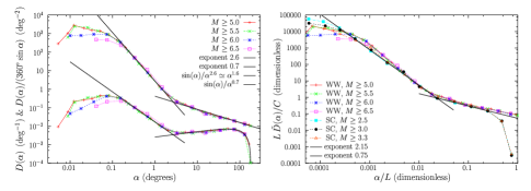
Figure 1: (color online) (a) Probability densities of earthquake jumps, defined per unit distance (angle), $D(\alpha)$, and per unit solid angle, $\tilde{D}(\alpha)=D(\alpha)/(360^{\circ}\sin\alpha)$ (shifted up a factor 1000 for clarity sake), for worldwide seismicity with lower magnitudes from $M_{c}=5$ to $M_{c}=6.5$. Lines come from power-law fits to $\tilde{D}(\alpha)$ for $M_{c}=5$. (b) Rescaled probability densities $\tilde{D}(\alpha)$ for worldwide seismicity (WW) and for several stationary periods in Southern California (SC), with different $M_{c}$ values. For each case, $L=180^{\circ}$ and $L=6.5^{\circ}$, and the normalization factors $C=0.0235$ and $C=1.14$ degrees^-1 are determined for $M_{c}=5$ and $M_{c}=2.5$ disregarding the smallest jumps. Power-law fits for SC with $M_{c}=2.5$ are shown.

The results for the NEIC-PDE worldwide catalog PDE , covering the period 1973-2002, are shown in Fig. 1(a) (bottom set of curves), using events with magnitude $M$ above different thresholds $M_{c}$ (i.e., $M\geq M_{c}$). An important conclusion drawn from the figure is the independence of the jump distributions on the magnitude threshold, as in Ref. Davidsen_distance , implying that the spatial occurrence of large earthquakes is no different than the occurrence of small ones, in contrast to claims by some authors Molchan04 . There is, nevertheless, an exception for small distances, less than about $0.1^{\circ}$ ($\simeq 10$ km) for $M_{c}$ from 5.5 to 6, comparable with the size of rupture Davidsen_Grassberger . The distributions are characterized by a decreasing power-law regime from about $0.1^{\circ}$ to $2^{\circ}$, with an exponent about 1.6, and a possible increasing second power law for $\alpha>2^{\circ}$, with exponent 0.3, decaying abruptly close to the maximum distance. Note the difference between these exponents and the value 0.6, obtained in Ref. Davidsen_distance mixing many areas in Southern California and including non-stationary periods.

However, the measurement of $D(\alpha)$ contains an inconsistency when it is used for distances over a sphere; for instance, after any event, there are many ways to obtain a jump of $\alpha=90^{\circ}$ (360 “ways” in intervals of $1^{\circ}$) but there is only one way to get $\alpha=180^{\circ}$ (which is the maximum possible distance, corresponding to the antipodes of the initiating event). Therefore, instead of working with the probability density defined per unit distance, i.e., per unit angle, it is preferable to use (and easier to interpret) the probability density defined per unit solid angle (taking into account all the possible orientations for a given distance $\alpha$). A straightforward way to estimate this quantity is by means of the transformation

$$D(\alpha)\rightarrow\tilde{D}(\alpha)\equiv{D(\alpha)}/{(2\pi\sin\alpha)},$$

due to the fact that $2\pi\sin\alpha\,d\alpha$ is the element of solid angle defined by the points at distance $\alpha$.

The results of the transformation are clearly seen in Fig. 1(a) (top curves). In addition to the power law for the range $0.1^{\circ}-2^{\circ}$, whose exponent turns out to be $\sim 2.6$, the second power law, now decreasing, becomes more apparent from about $2^{\circ}$ to the maximum distance, $180^{\circ}$, with an exponent $\sim 0.7$. This second power law seems to imply a dependence of events at large spatial scales. Indeed, for a given direction, it is more likely a jump with $\alpha=20^{\circ}$ than one of $160^{\circ}$ (independence would imply that the probabilities were the same); however, this effect is due to the fact that earthquake occurrence is not uniform over the Earth but fractal, and the power law reflects the fractal structure of the epicenters. If for long distances there is no causal relation between events, the distribution of earthquake jumps is equivalent to the distribution of distances between any pair of earthquakes (not necessarily consecutive); and as the density corresponding to this distance (per unit distance) is the derivative of the well-known correlation integral, widely used to obtain fractal dimensions, independence at long distances implies

$$D(\alpha)\sim\alpha^{d_{f}-1}\,\mbox{ and }\tilde{D}(\alpha)\sim 1/\alpha^{2-d_{f}}\,\mbox{ for long $\alpha$,}$$

where $d_{f}$ is the correlation dimension. We have measured the probability density of the distance between any two earthquakes (per unit solid angle), obtaining a behavior proportional to $1/\alpha^{0.85}$, for events with $M\geq 6$, which implies a correlation dimension $d_{f}\simeq 1.15$ in reasonable agreement with $\tilde{D}(\alpha)\sim 1/\alpha^{0.7}$, and confirming the independence of events for $\alpha>2^{\circ}$.

Turning back to the short-jump regime, the excess of probability given by the corresponding power-law with respect the long-jump power law (associated to the uncorrelated regime) is a clear sign of spatial clustering in earthquake occurrence, extending up to distances of about $2^{\circ}\simeq 200$ km. It is likely that this clustering extends beyond this limit, but it is not detectable with this procedure as it is hidden below the uncorrelated, long-distance regime. In any case, the power law behavior implies the no existence of a finite correlation length, at least up to 200 km, at variance with the findings of Ref. Huc_Main ; McKernon . In consequence we can consider the earthquake jumps as Lévy flights, which are one of the main causes of anomalous diffusion.

In contrast to worldwide seismicity, regional seismicity turns out to be nonstationary, in general, and in the same way as for waiting-time distributions Corral_prl.2004 , the distributions of earthquake jumps depend on the time window selected for analysis. This problem will be avoided here by considering specific time windows characterized by stationary seismicity; an important realization then is that stationary seismicity is characterized by stationary distributions. Additionally, stationary seismicity has the advantage of a lower magnitude threshold of completeness, due to the absence of large events.

We consider Southern-California seismicity, from the waveform cross-correlation catalog by Shearer et al. Shearer . The analysis has been performed on 11 stationary periods, comprised between the years 1986 and 2002, yielding a total time span of 9.25 years and containing 6072 events for $M\geq 2.5$. It is very striking, as Fig. 1(b) shows, that the distributions of jumps resemble very much those of the worldwide case, with two power-law regimes, but in a different scale (the separation is at about $0.1^{\circ}$). In principle, for a smaller area such as California one would expect that the distribution of jumps is just a truncation of the global one, but Fig. 1(b) clearly refutes this fact, providing a clear illustration of earthquake-occurrence self-similarity in space. In fact, the figure shows these distributions rescaled by a factor $L$, with $L$ the maximum distance for the region, which is $L\simeq 6.5^{\circ}$ for Southern California. and $L=180^{\circ}$ for the worldwide case (also included in the plot). The reasonable data collapse is a signature of the existence of a scaling law for the jump distribution,

$$D(\alpha)\simeq g(\alpha/L)/L$$

(for $\tilde{D}(\alpha)$ we need to include an extra factor $C$ of normalization). The scaling law can only be given the status of approximated, as the exponent for short jumps for Southern California seems to be different than in the worldwide case, 2.15 versus 2.6 for the distribution $\tilde{D}$. Nevertheless, this variation could be due to artifacts in the short-distance properties of the catalogs. On the other hand, the long-jump regime is well described by the worldwide exponent. We recall that the exponents are far from the value of Davidsen and Paczuski for the nonstationary California case Davidsen_distance . The main difference with the worldwide case is the abrupt decay of $\tilde{D}(\alpha)$ close to the maximum $\alpha$. Clearly, this is a boundary effect. We have tried several corrections for this effect (in particular the factor $2\pi\sin\alpha$ is not right when the ring defined by the set of points at a distance $\alpha$ is not totally included in the region under study) but we have not found a substantial improvement and then we have preferred to keep the things simple.

The distributions of jumps we have obtained, together with previous work on the distribution of waiting times Corral_prl.2004 , provide a simple picture of earthquake occurrence as a continuous-time random walk. This means that we can understand seismic activity as a random walk over the Earth surface, where one event comes after another at a distance that follows $D(\alpha)$ and after a waiting time $\tau$ given by the waiting-time probability density, $D(\tau)$. However, an important ingredient is missing in this picture, as we need to take into account the correlations between distances and waiting times.

With this goal in mind, we introduce the conditional waiting-time probability density, $D(\tau\,|\,X)$, where $|\,X$ means that only the cases where $X$ is verified are taken into account; in our case $X$ will be a set of values of the jumps. It turns out that if $D(\tau\,|\,X)$ does not depend on $X$, then $\tau$ and $X$ are independent, whereas when $D(\tau\,|\,X)$ changes with $X$, then $\tau$ and $X$ are correlated (nonlinearly, in general).

From the behavior of $D(\alpha)$, a natural threshold for the jumps in the worldwide case is $\alpha\simeq 2^{\circ}$. Figure 2(a) compares $D(\tau\,|\,\alpha\mbox{ short })$ with $D(\tau\,|\,\alpha\mbox{ long })$ for worldwide seismicity, where short and long refer to sets of distances below and above $2^{\circ}$, respectively. The differences are clear: for short jumps the waiting-time distribution is a decreasing power law for several decades, with an exponent close to 1, and ends in an exponential decay. We can identify these distributions with highly correlated events, i.e., aftershock sequences. On the other hand, for long $\alpha$ the waiting-time distribution seems to be exponential for its full range, compatible with a Poisson process and therefore with independent occurrence.

But more surprising than the differences between short and long jumps are perhaps the similarities for short jumps. In fact, there seems to be a radical change of behavior separated by $\alpha\simeq 2^{\circ}$, in the sense that if we are above, or below, this value, the distributions do not change, in other words, $D(\tau|\alpha<0.25^{\circ})=D(\tau|0.25\leq\alpha<1^{\circ})$, etc. and $D(\tau|2^{\circ}\leq\alpha<30^{\circ})=D(\tau|\alpha\geq 100^{\circ})$, etc., see Fig. 2(a) (for the range between $1^{\circ}$ and $2^{\circ}$ the behavior is not clear as the statistics is low). This means that for short jumps the waiting-time distribution is independent on the value of the jump, and the same happens for long jumps, but when the whole range of jumps is considered this is no longer true and both variables become dependent, in contrast to Ref. Davidsen_distance . For each set of curves we can fit a gamma distribution, $D(\tau|\alpha)\propto e^{-\tau/a}/\tau^{1-\gamma}$, turning out to be $\gamma\simeq 0.17$ for short $\alpha$ and $\gamma\simeq 0.9$ for long $\alpha$. The latter value is very close to 1, the characteristic value of a Poisson process; in fact, the difference between 1 and 0.9 is not significant within the uncertainty of our data, but if the hypothesis of a Poisson process for long distances could be rejected at any reasonable significance level (for which much more data would be necessary) and a value $\gamma<1$ could be significantly established, this would constitute a support for the existence of long-range earthquake triggering. In any case, our findings are in disagreement with the hypothesis put forward in Ref. Huc_Main , which considers seismicity as a process uncorrelated in time but correlated in space.

This result confirms that the universal scaling law found for stationary seismicity in Ref. Corral_prl.2004 is in fact a mixture of aftershocks and independent events, turning out to be very striking that this mixture leads to a universal behavior. The reason could be a universal proportion of aftershocks versus mainshocks in stationary seismicity Hainzl_bssa . Further, the conditional time distributions verify a scaling law,

$$D(\tau|\alpha_{\pm})=R(\mathcal{R},M_{c})f_{\pm}(R(\mathcal{R},M_{c})\tau),$$

where the indices $+$ and $-$ refer to long and short jumps, respectively, and $R^{-1}(\mathcal{R},M_{c})$ is the mean waiting time of the unconditional distribution for the region $\mathcal{R}$ and $M\geq M_{c}$ (obviously, a scaling with the mean of the conditional distribution also holds). Figure 2(b) shows this behavior.

The next step is to measure earthquake diffusion directly from data. The fundamental quantity is $p(\alpha,t)$, which we call diffusion profile and gives the probability density that two earthquakes (not consecutive) are at a distance $\alpha$ when they are separated by a time $t$, i.e.,

$$p(\alpha,t)d\alpha\equiv{\mbox{Prob}[\alpha\leq\mbox{ distance at a time }t<\alpha+d\alpha}].$$

In practice, the single value of $t$ is replaced by a range of values and, as above, we introduce $\tilde{p}(\alpha,t)\equiv p(\alpha,t)/(2\pi\sin\alpha)$. In the case of normal diffusion $\tilde{p}(\alpha,t)$ is given by a Gaussian distribution (more precisely, a semi-Gaussian, as $\alpha>0$), with a second moment scaling as $\langle\alpha^{2}\rangle\sim t$, whereas $p(\alpha,t)$ is given by a Rayleigh distribution (or a Maxwell distribution in three dimensions). In contrast, our measurements yield to results far from normality, see Fig. 3. For short times, the profile resembles the distribution of jumps with 2 regimes; as time evolves events migrate farther from the origin, towards the long-range part of the curve, which becomes dominant for all $\alpha$ for long times, with an exponent of value 0.8 for $\tilde{p}$.

A scaling law also holds for the diffusion profile, i.e.,

$$p(\alpha,t)=h(\alpha/L,t)/L.$$

Finally, the process turns out to be clearly subdiffusive, as $\langle\alpha^{2}\rangle$ grows more slowly than linearly, although we cannot provide a definite value of a exponent as in Refs. Marsan00 ; Helmstetter_jgr03 .

This paper would not have been possible without the effort of the researchers who have made earthquake catalogs publicly available. The Ramón y Cajal program and the projects BFM2003-06033 (MCyT) and 2001-SGR-00186 (DGRGC) are acknowledged.

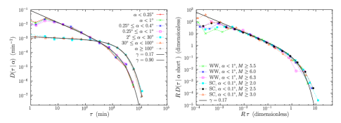
Figure 2: (color online) (a) Waiting-time probability densities conditioned to different sets of values of the jumps, in particular $\alpha$ short (below $1^{\circ}$) and $\alpha$ long (above $2^{\circ}$), using worldwide seismicity with $M\geq 5.5$. In each case, gamma fits to all the curves are shown, with parameter $\gamma=0.17$ ($\alpha$ short) and $\gamma=0.90$ ($\alpha$ long). (b) Rescaled waiting-time probability densities conditioned to short jumps, $\alpha<1^{\circ}$ for worldwide seismicity (WW) and $\alpha<0.1^{\circ}$ for Southern California (SC). Different $M_{c}$ values are used. The rescaling factor $R$ refers to the unconditional distribution, and only depends on $M_{c}$ and on the spatial region $\mathcal{R}$. The solid line is the gamma fit in (a) rescaled in the same way.

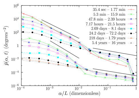
Figure 3: (color online) Diffusion profile $\tilde{p}(\alpha,t)$ versus $\alpha$ (rescaled by $L$) for worldwide seismicity with $M\geq 5.5$ (bottom curves) and for Southern California with $M\geq 2.5$ (top). Time ranges from tens of seconds to several years. The displayed power laws are indicative, and have the same exponents as the jump distributions.

References

- (1) S. Stein and M. Wysession. An Introduction to Seismology, Earthquakes, and Earth Structure. Blackwell Pub., 2003.
- (2) Y. Y. Kagan. Physica D, 77:160–192, 1994.
- (3) D. L. Turcotte. Fractals and Chaos in Geology and Geophysics. Cambridge University Press, 1997.
- (4) T. Utsu. International Handbook of Earthquake and Engineering Seismology, Part A. W. H. K. Lee, H. Kanamori, P. C. Jennings, and C. Kisslinger, eds., Academic Press, 2002.
- (5) D. Schorlemmer and S. Wiemer. Nature, 434:1086–1086, 2005.
- (6) D. Schorlemmer, S. Wiemer, and M. Wyss. Nature, 437:539–542, 2005.
- (7) P. A. Reasenberg and L. M. Jones. Science, 243:1173–1176, 1989.
- (8) P. Bak, K. Christensen, L. Danon, and T. Scanlon. Phys. Rev. Lett., 88:178501, 2002.
- (9) A. Corral. Phys. Rev. E, 68:035102, 2003.
- (10) A. Corral. Physica A, 340:590–597, 2004.
- (11) A. Corral and K. Christensen. http://arxiv.org/cond-mat/0509061, 2005.
- (12) A. Corral. Phys. Rev. Lett., 92:108501, 2004.
- (13) A. Corral. Phys. Rev. Lett., 95:028501, 2005.
- (14) K. Ito. Phys. Rev. E, 52:3232–3233, 1995.
- (15) S. Abe and N. Suzuki. J. Geophys. Res., B 108:2113, 2003.
- (16) J. Davidsen and M. Paczuski. Phys. Rev. Lett., 94:048501, 2005.
- (17) See http://wwwneic.cr.usgs.gov/neis/epic/epicglobal.html.
- (18) G. Molchan and T. Kronrod. On the frequency-magnitude law for fractal seismicity. http://arxiv.org/physics/0409142, 2004.
- (19) J. Davidsen, P. Grassberger, and M. Paczuski. Geophys. Res. Lett., (submitted), 2005.
- (20) M. Huc and I. G. Main. J. Geophys. Res., 108 B:2324, 2003.
- (21) C. McKernon and I. G. Main. J. Geophys. Res., 110:B05S05, 2005.
- (22) P. Shearer, E. Hauksson, G. Lin, and D. Kilb. Eos Trans. AGU, 84(46):Fall Meet. Suppl., Abstract S21D–0326, 2003. http://www.data.scec.org/ftp/catalogs/SHLK/.
- (23) S. Hainzl, F. Scherbaum, and C. Beauval. Bull. Seismol. Soc. Am., submitted, 2005.
- (24) D. Marsan, C. J. Bean, S. Steacy, and J. McCloskey. J. Geophys. Res., 105 B:28081–28094, 2000.
- (25) A. Helmstetter, G. Ouillon, and D. Sornette. J. Geophys. Res., 108 B:2483, 2003.