Full quantum distribution of contrast in interference experiments between interacting one dimensional Bose liquids

Abstract

We analyze interference experiments for a pair of independent one dimensional condensates of interacting bosonic atoms at zero temperature. We show that the distribution function of fringe amplitudes contains non-trivial information about non-local correlations within individual condensates and can be calculated explicitly using methods of conformal field theory. We point out interesting relations between these distribution functions, the partition function for a quantum impurity in a one-dimensional Luttinger liquid, and transfer matrices of conformal field theories. We demonstrate the connection between interference experiments in cold atoms and a variety of statistical models ranging from stochastic growth models to two dimensional quantum gravity. Such connection can be used to design a quantum simulator of unusual two-dimensional models described by nonunitary conformal field theories with negative central charges.

I Introduction

The hallmark of a Bose-Einstein condensate (BEC) is the existence of a well defined macroscopic phase. Indeed experiments with large condensates display robust matter wave interference with negligible fluctuations in the fringe contrast ketterle . From this point of view, large three dimensional condensates may be thought of as classical objects. However, there is a continuous range of possibilities intermediate between perfect condensates on one side and systems that do not display an interference pattern, like high temperature thermal gases, on the other pad . For example, one-dimensional interacting bosons display interference patterns with a reduced contrast and with non negligible shot to shot fluctuations of the fringe contrast schmiedmayer . In this paper we analyze the full distribution associated with this quantum noise, and discuss what it can tell us about the underlying strongly correlated state.

By virtue of its direct connection to the concepts of quantum measurement, study of quantum noise has deepened our understanding in a variety of areas. Understanding the noise in photo detection photon prompted the creation of nonclassical states of light and led to the development of quantum optics. In mesoscopic electron systems, current fluctuations contain information that is not available in simple transport measurements. For example, they can be used to distinguish electrical resistance due to diffusive scattering from the resistance due to point contact tunneling (see Ref. [meso, ] for a review). Single atom detectors have been used recently to perform Hanburry-Brown-Twiss experiments with cold atoms Esslinger ; Aspect . Finally, analysis of noise correlations in time of flight experiments of ultra cold atoms has been proposed pra and tested greiner ; bloch , promising a powerful new technique to access many-body correlations in such systems. In these applications, the quantities of direct interest are contained in the first few moments of the noise distribution, such as the noise power spectrum. However deeper insights into quantum systems may be gained by obtaining the full statistics of the fluctuations.

One of the central problems in the field of ultra cold atoms is finding new ways of characterizing many-body quantum states. In this paper we demonstrate that analysis of the distribution function of contrast in interference experiments between interacting one dimensional Bose liquids provides a novel probe of non-local correlations and entanglement present in these systems. It is known that the average amplitude of interference fringes can be used to extract two point correlation functions in fluctuating condensates pad . This idea has been successfully employed by Hadzibabic et al. to measure the Kosterlitz-Thouless transition in two dimensional systems hadzibabic . Interference experiments, however, contain more information than the average value of the contrast. Each observation of the interference pattern is a classical measurement of a quantum mechanical state, so the result of each individual measurement will be different from the average value. As we discuss below, higher moments of the distribution function of interference amplitudes correspond to high order correlation functions. Hence the knowledge of the entire distribution function reveals global properties of the system that depend on non-local correlation functions of arbitrarily high order. So far, the discussion of full counting statistics has been limited mainly to systems of non interacting particles levitov . The main result of this paper, by contrast, is an expression for the full distribution of amplitudes of interference fringes arising from one dimensional interacting Bose liquids, that can be described by a Luttinger liquid.

The approach used in this paper for analyzing interference experiments can be generalized to a variety of other measurements in cold atom systems. For example, one can analyze fluctuations in particle number in systems with pairing belzig and fluctuations in magnetization in Mott states of atoms with magnetic exchange interactions. In both cases distribution functions will contain non-trivial information about underlying many-body states. One can also consider time dependent phenomena such as evolution of phase coherence between a pair of condensates coupled by a finite tunneling amplitude schmiedmayer . In this paper we focus on the distribution function of contrast in interference experiments between independent Bose liquids in their ground states. Already in this case we find a non-trivial evolution of the distribution function from the non-fluctuating perfect contrast for the case of non-interacting atoms to the Poissonian distribution of contrast for atoms in the regime of infinitely strong repulsion. We think that our work constitutes one of the first steps in the direction of developing a new method for characterizing interacting many-body quantum states of cold atoms using full distribution function of some extensive quantum operator, such as the total magnetization or the interference amplitude operator defined in equation (1). Different kinds of cold atom systems and experimental probes can be studied following this general approach.

We start our analysis by establishing the relation between the probability distribution function of the interference amplitude and the partition function of a boundary sine-Gordon model. Using methods of conformal field theory, we reduce this problem to that of finding a spectral determinant of a simple one-dimensional, single-particle Schrödinger equation. We solve this problem numerically, as well as analytically using the WKB approximation, to obtain the desired fringe distribution for any value of the Luttinger parameter.

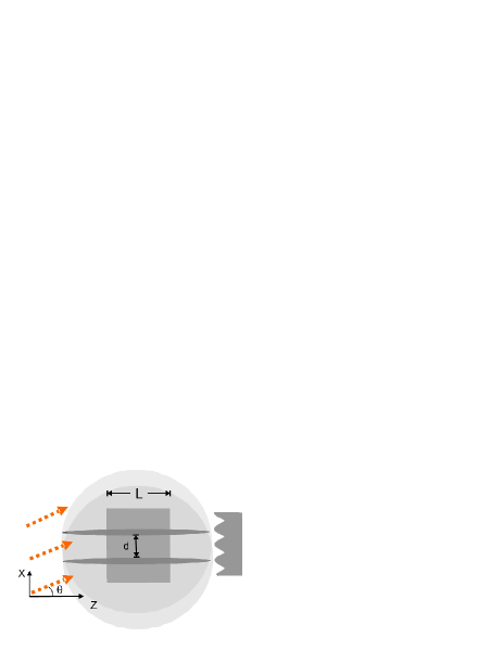
Figure 1: Schematic view of the possible experimental setup, which produces interference pattern between two independent 1D condensates.

It is interesting to point out that one can take the alternative point of view on the relation between interference experiments with BEC and the quantum impurity problem. By measuring the distribution function of the interference amplitudes experimentally one obtains the full partition function of the boundary Sine-Gordon problem (see eq. (6) below). This model describes a range of interesting problems such as an impurity in a Luttinger liquid kanefisher , the asymmetric Kondo model FLS2 , and the tunneling of a particle in the presence of dissipation within a Caldeira-Leggett approach caldeira-leggett . As we discuss below, interference experiments can be used to obtain the partition function of these systems not only in the ground state but also in the non-equilibrium regimes (e.g. in the presence of a finite voltage). Hence interference experiments can be considered as a quantum solver of these non-trivial many-body problems.

Another surprising implication of our analysis is that interference experiments with one dimensional cold atoms can be used as a quantum simulator of several fundamental problems in physics. This connection relies on the fact that many models of systems with critical behavior in two-dimensional statistical mechanics, one dimensional field theories and many-body quantum systems can be described by continuum theories with conformal invariance. Basic ingredients of any conformal field theory are the central charge and conformal dimensions of operators. One dimensional quantum systems of interacting particles have positive central charges and correspond to the so-called unitary class. On the other hand, there is a non-unitary class of models which have negative central charges. Such models appear in contexts as different as two dimensional quantum gravity and stochastic growth models and they have very unusual properties (see e.g. Ref. [difrancesco, ]). In this paper we demonstrate that interference experiments with one dimensional condensates can be used to analyze models in nonunitary universality class by virtue of the exact mathematical relation between the distribution function of interference amplitude and the so-called Q-operators of conformal field theories. In Fig. 4 below we show a diagram which illustrates several models that can be studied using interference experiments.

II Full Quantum Distribution of the Interference Contrast

The setup for the interference experiments we consider is sketched in Fig. 1. Two independent quasi-condensates are allowed to expand in the transverse direction. After sufficient time of expansion, the integrated density profile is measured by the imaging beam which is sent at an angle ${\theta}$ to the condensate axis. This setup is quite common for the interference experiments in cold atoms and was already realized by several groups [hadzibabic, ; schumm, ].

Everywhere in this paper we consider the two condensates to be identical, although our analysis can be generalized to the case of different condensates (see also Ref. [niu, ]). We assume that before the expansion, atoms are confined to the lowest transverse channels of their respective traps and that the optical imaging length $L$ (which is smaller than or equal to the size of the system in the axial direction) is much larger than the coherence length of the condensates. This allows us to use an effective Luttinger liquid description of the interacting bosons cazalilla . The operator corresponding to the interference signal of the two condensates pad is given by

$$A_{\tilde{p}}=\!\!\int_{0}^{L}\!\!dz\,a_{1}^{\dagger}(z)\,a_{2}(z)\,\mathrm{e}^{i\tilde{p}z}.$$ (1)

Here $a_{1}$ and $a_{2}$ are the bosonic operators in the two systems before the expansion, and the integrals are taken along the condensates. The seeming winding of the relative phase between the two systems, described by the exponential term in equation (1), can either come from the measurement process itself or from the actual motion of the condensates pad . If the condensates are at rest, we have $\tilde{p}=\left(md/\hbar t\right)\tan{\theta}$, where $m$ is the atom’s mass, $d$ is the separation between the two condensates and $t$ is the time when the measurement was done after the free expansion started. With some abuse of terminology we will call $\tilde{p}$ the relative momentum. When condensates one and two are independent, one finds that the expectation value of $\langle A_{\tilde{p}}\rangle$ vanishes, however $\langle|A_{\tilde{p}}|^{2}\rangle$ is finite. This means that individual measurements show a finite amplitude of interference fringes, however their phase is completely unpredictable. Higher moments of the interference fringe amplitude are given by pad

$$\langle|A_{\tilde{p}}|^{2n}\rangle=A_{0}^{2n}Z_{2n}^{(p)},\;\mbox{where}\;A_{0}=\sqrt{C\rho\,\xi_{h}^{1/K}L^{2-1/K}},$$ (2)

where $C$ is a constant of order unity, $\rho$ is the particle density in each condensate, $\xi_{h}$ is the short range cutoff equal to the healing length, and $K$ is the Luttinger parameter describing the interaction strength. In this letter we assume that $K>1$, which is always the case for bosons with $\delta$-function type repulsive interactions note1 . Coefficients $Z_{2n}$ in Eq. (2) are given bynote :

$$Z_{2n}^{(p)}(K)=\int_{0}^{2\pi}\!\dots\!\int_{0}^{2\pi}\prod_{i=1}^{n}{du_{i}\over 2\pi}{dv_{i}\over 2\pi}e^{i2p\sum_{i}(u_{i}-v_{i})}$$

$$\left|{\prod_{i<j}2\sin\left({u_{i}-u_{j}\over 2}\right)\prod_{k<l}2\sin\left({v_{k}-v_{l}\over 2}\right)\over\prod_{i,k}2\sin\left({u_{i}-v_{k}\over 2}\right)}\right|^{1/K},$$ (3)

where $p$ is the relative momentum measured in units of $2\pi/L$: $p=\tilde{p}L/2\pi$.

Coefficients $Z_{2n}^{(p)}$ originally appeared in the grand canonical partition function of a neutral two-component Coulomb gas on a circle

$$Z_{p}(K,x)=\sum_{n=0}^{\infty}{x^{2n}\over(n!)^{2}}Z_{2n}^{(p)}(K).$$ (4)

Here $x$ is the fugacity of Coulomb charges and $Z_{2n}$ describe contributions from configurations with $2n$ charges (i.e. canonical partition functions). The partition function (4) with $K>1$ and $p$ being half-integer describes several problems in statistical physics (see Ref. [FLS1, ] and references therein). In particular, it describes an impurity in a one-dimensional interacting electron liquid. At low energies this problem is described by a Luttinger liquid (LL) with an additional local non-linear term due to backscattering from the impurity:

$$S={\pi K\over 2}\int_{-\infty}^{\infty}dy\int_{0}^{\beta}d\tau\,\left[(\partial_{\tau}\phi)^{2}+(\partial_{y}\phi)^{2}\right]$$

$$~{}~{}~{}~{}~{}~{}~{}~{}~{}~{}~{}~{}~{}~{}~{}~{}~{}+2g\int_{0}^{\beta}d\tau\,\cos\left[2\pi\phi(0,\tau)+\frac{p}{\beta}\tau\right],$$ (5)

where $g$ is the amplitude of backscattering on the impurity and $\phi(x)$ is a bosonic phase field associated with the electron field operator $\psi(x)\sim e^{i\phi}$. In the bosonized form the electron-electron interaction becomes quadratic and is effectively described by the Luttinger parameter $K$. Perturbative expansion of the corresponding partition function in powers of $g$ produces the series (4) with the fugacity given by $x=g\,\beta(2\pi/\beta\kappa)^{1/2K}$. Here $\kappa$ is a non-universal renormalization factor, which sets the scale for the long distance asymptotics of the correlation functions: $\langle\exp[2i(\phi(x,\tau)-\phi(0,0))]\rangle\sim(\kappa\sqrt{x^{2}+\tau^{2}})^{-1/K}$. Finally, the single impurity Kondo model is related to $Z_{p}(K,x)$ as well FLS2 .

It is easy to understand the origin of the relation between interference experiments and a quantum impurity problem. Moments of fringe amplitudes are determined by high order correlation functions computed at the same time but in different points in space. On the other hand, expansion of the partition function for a quantum impurity contains correlation functions computed at the same spatial point but at different times. Lorentz invariance of the LL ensures that the two are the same. Note that the analogue of the finite imaging angle $\theta$ in the interference experiments is a finite voltage in the quantum impurity problem bazhanov98 . This analogy can be also understood from the interchanged roles of space and time in the two systems.

When describing interference experiments it is convenient to define the normalized amplitude of interference fringes ${\alpha}=A_{\tilde{p}}^{2}/A_{0}^{2}$. From eq. (2) we find that $\langle{\alpha}^{n}\rangle=Z^{(p)}_{2n}$, so by measuring the distribution function $W_{p}({\alpha})$ experimentally, we get direct access to the partition function (4). We point out that $W_{p}({\alpha})$ can be used to compute all moments of $A_{\tilde{p}}^{2}$, and therefore contains information about high order correlation functions of the interacting Bose liquids.

Using Taylor expansion of the modified Bessel function as well as Eq. (4) and the fact that $\langle{\alpha}^{n}\rangle=Z^{p}_{2n}$ we find

$$Z_{p}(K,x)=\int_{0}^{\infty}W_{p}({\alpha})\,I_{0}(2x\sqrt{{\alpha}})\,d{\alpha}.$$ (6)

Inverting Eq. (6) we can express the probability $W_{p}({\alpha})$ through the partition function $Z_{p}(K,x)$. Noting that $I_{0}(ix)=J_{0}(x)$ and using the completeness relation for Bessel functions, $\int_{0}^{\infty}J_{0}(\lambda x)J_{0}(\lambda y)|x|\lambda d\lambda=\delta(|x|-|y|)$, we obtain

$$W_{p}({\alpha})=2\int_{0}^{\infty}Z_{p}(K,ix)J_{0}(2x\sqrt{{\alpha}})xdx,$$ (7)

It is important that the last equation has the partition function at imaginary value of the coupling constant. This should be understood as analytic continuation of $Z_{p}(K,x)$.

There are several ways how one can compute $W_{p}({\alpha})$. The most straightforward approach is to evaluate the coefficients $Z_{2n}^{(p)}$ and thus determine all the moments of the distribution. Explicit expressions for $Z_{2n}^{(p)}$ can be obtained using orthogonal Jack-polynomials FLS1 . However, each of these coefficients is given as a series of products of $\Gamma$-functions and their evaluation becomes extremely cumbersome for $n\geq 3$. Another approach to finding $W_{p}({\alpha})$ is to compute $Z_{p}(K,x)$ using the thermodynamic Bethe Ansatz for the quantum impurity problem FLS1 . This method works only for half integer $K$ and requires solution of coupled integral equations. Besides, relating $Z_{p}(K,x)$ to the distribution function of interference amplitudes requires analytic continuation of $Z_{p}(K,x)$ into the complex plane, $x\to ix$ (see Eq. (7)), which introduces additional complications. In this paper we will use a different method, which is based on studies of the integrable structure of conformal field theories BLZ1-3 . In particular, it was shown that the vacuum expectation value of Baxter’s ${\bf Q}$ operator, central to the integrable structure of the models, coincides with the grand partition function of interest up to an overall prefactor BLZ1-3 (see supplementary material for more details):

$$Q_{p}^{\rm vac}(c,\lambda)=\lambda^{4p/K}Z_{p}(K,-ix),$$ (8)

where $x$ is related to the spectral parameter $\lambda$ as $x=\pi\lambda/\sin(\pi/2K)$ and the central charge $c=1-6(2K-1/(2K))^{2}$. It was conjectured in Refs. [DT, ,BLZ, ] that the vacuum expectation value $Q_{p}^{\rm vac}(\lambda)$ is proportional to the spectral determinant of the single particle Schrödinger equation

$$-\partial_{x}^{2}\Psi(x)+\left(x^{4K-2}+\frac{l(l+1)}{x^{2}}\right)\Psi(x)=E\Psi(x),$$ (9)

where $l=4pK-\frac{1}{2}$. So, $Q^{\rm vac}(\lambda)=\lambda^{4p/K}D(\rho\lambda^{2})$, where $\rho=(4K)^{2-1/K}\Gamma^{2}(1-1/2K)$, $D(E)$ is the spectral determinant defined as $D(E)=\prod_{n=1}^{\infty}(1-E/E_{n})$, and $E_{n}$ are the eigenvalues of (9). Thus, we get

$$Z_{p}(K,ix)=\prod_{n=1}^{\infty}\left(1-\frac{\rho\lambda^{2}}{E_{n}}\right).$$ (10)

To evaluate the distribution function we solve the Schrödinger Eq.(9) numerically. Details of the analytical treatment and comparison with numerics will be reported elsewhere ADGP . We checked the accuracy of the numerics as well as conjecture (10) by comparing coefficients $Z_{2}^{(p)}(K)$ and $Z_{4}^{(p)}(K)$ evaluated for various $K$ using (i) the spectral determinant (e.g. $Z_{2}^{(p)}\sim\sum 1/E_{n}$, $Z_{4}^{(p)}\sim(\sum 1/E_{n})^{2}-\sum 1/E_{n}^{2})$ ), and (ii) the exact expressions of Ref. [FLS1, ] based on Jack polynomials. We found perfect agreement between the two methods.

To compare distributions at different $K$ with each other it is convenient to use a normalized interference amplitude $\tilde{\alpha}={\alpha}/{\langle{\alpha}\rangle}=A^{2}/{\langle A^{2}\rangle}$ instead ${\alpha}$. This change of variable is also convenient for comparison with experiments. The distribution function $W_{0}(\tilde{\alpha})$ is shown in Fig. 2 for several values of $K$. For $K$ close to 1 (Tonks-Girardeau limit) $W_{0}$ is a wide Poissonian function, which gradually narrows as $K$ increases, finally becoming a narrow $\delta$-function at $K\to\infty$ (the limit of noninteracting bosons). Interestingly, the distribution function remains asymmetric for arbitrarily large $K$. In fact we find that $W_{0}(\tilde{\alpha}-1)$ tends to a universal scaling form, parameterized by a single number characterizing the width of the distribution: $\delta\tilde{\alpha}\equiv\sqrt{\langle\tilde{\alpha}^{2}\rangle-1}\approx\pi/\sqrt{6}K$ (see Ref. [pad, ]). We conjecture that this limiting form of $W_{0}$ is the Gumbel distribution Katzgraber , which frequently appears in problems of extreme value statistics Gumbel : $W_{0}(\tilde{\alpha}-1)\to W_{G}(\tilde{\alpha},K,\gamma)$, where $\gamma\approx 0.577$ is the Euler gamma-constant and

$$W_{G}(x,a,b)=a\exp\left(ax-b-\exp(ax-b)\right).$$ (11)

We plot the scaled distribution functions: $\delta\tilde{\alpha}\,W_{0}\left((\tilde{\alpha}-1\right)/\delta\tilde{\alpha})$. Note that $W_{0}$ was multiplied by ${\delta}\tilde{\alpha}$ to preserve the normalization condition (so that the total probability is equal to unity) for $K=10,20,40$. For comparison in Fig. 3 we also present the scaled Gumbel distribution. One can see that as $K$ increases the function $W_{0}$ indeed approaches to $W_{G}$. Gumbel distributions are frequently associated with random walks in strongly correlated systems Gumbel . Indeed one can view the interference signal in Eq. (1) as a sum of contributions coming from different points along the condensates. For weak interactions (large $K$) these contributions are strongly correlated because the phases of each of the condensates only weakly fluctuate along $z$. Thus there is no surprise that $W_{0}$ approaches the Gumbel distribution. One can also understand this result noting that for $K\gg 1$ the distribution function of the interference amplitude is dominated by rare events which reduce the contrast. The Gumbel distribution was introduced precisely to describe rare events such as stock market crashes or earthquakes. In supplementary materials (sec. V.2) we also discuss distribution functions for finite values of the observation angle (i.e. finite $p$).

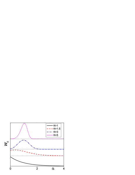
Figure 2: Evolution of the distribution function $W_{0}(\tilde{\alpha})$ for different values of $K$ at $p=0$. At larger values of $K$ the function $W_{p}$ tends to the delta-function (see text for details).

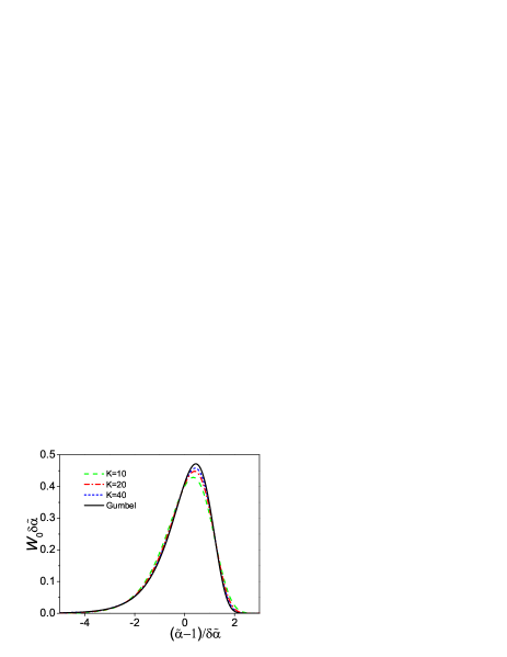
Figure 3: Scaled distribution function $\delta\tilde{\alpha}W_{0}\left((\tilde{\alpha}-1)/\delta\tilde{\alpha}\right)$, where $\delta\tilde{\alpha}$ is the width of the distribution, for large $K$. The function $W_{0}$ is multiplied by $\delta\tilde{\alpha}$ to preserve the total probability, which must be equal to unity. The dashed and dotted lines correspond to different values of $K$. The solid line corresponds to the conjectured Gumbel distribution.

Interestingly, the distribution function $W_{p}(\alpha)$ provides a very simple and convenient framework for describing both the partition function (4) and the expectation values of the $Q$-operator. Indeed, $W_{p}(\alpha)$ is a smooth well behaved function at all values of $K$ and it can be easily approximated by simple analytic expressions.

III Quantum simulation

As we mentioned earlier, the distribution function $W_{p}({\alpha})$ can be used to obtain the partition function $Z_{p}(K,x)$ (see Eq. (6)) describing a range of various problems like quantum impurity in a one-dimensional electron liquid, asymmetric Kondo problem, and dissipative tunneling. It is easy to see that momentum $p$ in the interference experiments corresponds to the external applied voltage in the impurity problem ($ip\sim V$). This follows from the interchanged roles of space and time in the two problems. Thus measuring $W({\alpha})$ experimentally and taking its integral transform one directly simulates these problems in or out of equilibrium. Moreover, after substituting $I_{0}(2x\sqrt{{\alpha}})\to J_{0}(2x\sqrt{{\alpha}})$ in Eq. (6) one obtains the partition functions of the above models with imaginary coupling constants. Such models have been actively investigated recently in the context of theories with PT-symmetric rather than Hermitean Hamiltonians bender .

The partition function with the imaginary coupling also gives the expectation values of the Baxter $Q$-operator (see Eq. (8)) corresponding to various conformal field theories (CFTs). In general, such theories are particularly important because many models of two-dimensional statistical mechanics, field theory, and many-body quantum systems at critical points can be described by some continuum theories having a property of conformal invariance. This leads to a description of critical systems on the basis of conformal field theory, which basic ingredients are the central charge and conformal dimensions. This set of data classify different universality classes, which often describe very different physical models. The property of positivity of the central charge leads to a unitary theory. Physically, the central charge determines the vacuum (Casimir) energy of the system and governs the finite-size scaling effects. On the other hand there is a class of models whose universality classes of critical behavior are described by the conformal-invariant models with negative central charges. These theories are nonunitary and their properties are thus very different from those described by positive central charges.

Conformal field theories corresponding to Eq. (8) are characterized by negative central charge $c=1-6(2K-1/(2K))^{2}$ and the highest weight $\Delta=(2pK)^{2}+(c-1)/24$ (see Ref. [BLZ1-3, ]). These relations give $c\leq-2$ for $K\geq 1$. Theories with negative central charges appear in different contexts of statistical mechanics, stochastic growth models, 2D quantum gravity, models of 2D turbulence and even high-energy QCD. In particular, $c=-2$ CFT has the field-theoretical representation in terms of the ghost (anticommuting) fields and also corresponds to the critical behavior of the non-intersecting loop model on a 2D lattice Nienhuis as well as to the special case of the stochastic Loewner evolution equation, describing the growth of random fractal stochastic conformal-invariant interface (see e.g. Ref. [Cardy, ]). The classic example of CFT with negative $c$ is the Yang-Lee singularity $c=-22/5$ describing the critical behavior of the Ising model in imaginary magnetic field. Models of 2D quantum gravity described by the fluctuating lattice geometry are related to negative $c$ as well. Possibly, the high-energy limit of multicolor QCD is described by the integrable CFT with negative (or zero) central charge Lipatov . We illustrate the dependence of $c$ on $K$ as well as particular examples of models corresponding to different values of $c$ in Fig. 4.

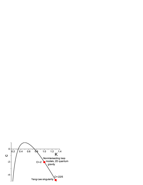
Figure 4: Dependence of the central charge of conformal field theories corresponding to interference experiments on the Luttinger liquid parameter $K$. The red circles correspond to some particular examples discussed in the text.

The spectrum of $Q$-operator can be used to reconstruct the transfer matrices of the above mentioned negative $c$ models. Particular example of such procedure for $c=-2$ universality class was explicitly constructed in Ref. [BLZ1-3, ]. In this case only the vacuum expectation value was needed to reconstruct the whole transfer matrix. The transfer matrices contain all the information about the properties of underlying models. In this sense interference experiments simulate these models. Experimentally, the central charge can be tuned by varying the interaction $K$ and the scaling dimensions $\Delta$ of corresponding physical operators can be manipulated by changing the observation angle $p$. An interesting challenge here is the experimental determination of nonvacuum values of the ${\bf Q}$ and ${\bf T}$ operators. This is an open question.

Needless to say that the range of models mentioned above, which belong to nonunitary universality classes is difficult (if possible at all) to realize by other ways. The interference of condensates provides a possible and a plausible way to explore the interesting physics of various models ranging from statistical to high energy physics.

IV summary

To summarize, in this paper we analyzed interference experiments between two independent one dimensional quasi-condensates. We computed the distribution function of the amplitude of interference fringes relating this problem to the properties of $Q$ operators of conformal field theories with negative central charges. We showed how one can use the distribution function of the interference amplitude to reconstruct the partition function of a two-dimensional Coulomb gas confined to a circle. This partition function is related to a variety of statistical and field-theoretical models. Thus studying the interference distribution function experimentally, one can directly simulate these interesting models.

We considered only a particular example of interference between two one-dimensional condensates and showed the connection between the distribution function of fringe amplitudes and the properties of various models. This analysis can be extended to other systems with quasi long-range order, e.g. to two-dimensional Bose systems at finite temperature. One can expect that there will be analogous connections to different classes of problems, some of which might not be exactly solvable. The interference experiments open new ways of solving these problems by direct simulation of the underlying models.

We are grateful to I. Affleck, C. Bender, P. Fendley, V. M. Galitski, M. Greiner, Z. Hadzibabic, H. Katzgraber, M. Lukin, S. L. Lukyanov, M. Oberthaller, M. Oshikawa, M. Pletyukhov, J. Schmiedmayer, V. Vuletic, D. Weiss, K. Yung and A. B. Zamolodchikov for useful discussions. This work was partially supported by the NSF grant DMR-0132874. V.G. is supported by Swiss National Science Foundation, grant PBFR2-110423.

V Supplementary material

V.1 Mathematical details

Function $Z(K,g)$ can be computed using the Thermodynamic Bethe Ansatz. This was used in Refs. [FLS1, ; FLS2, ] to evaluate the current through a boundary impurity. However to compute the distribution function $W$ we need analytic continuation of the partition function $Z(K,ig)$. Expression for $Z(K,g)$ is given as a solution of coupled integral equations and performing its analytic continuation is not easy. In this paper we use an alternative approach.

In a recent series of papers Bazhanov, Lukyanov, and Zamolodchikov explored an integrable structure of conformal field theories focusing on connections to solvable problems on lattices BLZ1-3 . Key ingredients of solvability of lattice models are is the so-called transfer matrix ${\bf T}(\lambda)$ operators. These operators contain information about all integrals of motion as well as excitation spectra of the system. Transfer matrices are defined as a function of the so-called spectral parameter $\lambda$ (in the continuum limit $\lambda$ corresponds to rapidity) and commute for different values of $\lambda$. The latter property is a direct manifestation of the existence of infinite number of commuting integrals of motion. In his studies of 8-vertex model, BaxterBaxter introduced the operator ${\bf Q}(\lambda)$ which helps to find an eigenvalues of ${\bf T}$. Operators ${\bf T}$ and ${\bf Q}_{\pm}$ satisfy a set of commutation relations, in particular BLZ1-3

$${\bf T}(\lambda){\bf Q}_{\pm}(\lambda)={\bf Q}_{\pm}(q\lambda)+{\bf Q}_{\pm}(q^{-1}\lambda)$$ (12)

where $q=\exp(i\pi/2K)$. So $T$ matrices can be obtained explicitly when one knows the Q operators.

Operators ${\bf A}_{\pm}(\lambda)={\bf Q}_{\pm}(\lambda)\lambda^{\mp 4p/K}$ act in the representation space of Virasoro algebra, which can be constructed from the Fock space of bosonic operators $a_{\pm n}$ satisfying $a_{n}|p\rangle=0$, $(n>0)$. The Fock vacuum state $|p\rangle$ is an eigenstate of the momentum operator, $P|p\rangle=p|p\rangle$. For $p=N/2$ ($N=0,1,2...$) the vacuum eigenvalues of the operator ${\bf A}_{\pm}(\lambda)$, ${\bf A}_{\pm}(\lambda)|p\rangle=A_{\pm}^{(vac)}|p\rangle$, are given by ( below we consider only the quantities with the $+$ subscript which correspond to the positive $p$)

$$A^{(vac)}(\lambda)=Z_{p}(K,-ix)$$ (13)

where

$$\lambda=\frac{x}{\pi}\sin\left(\frac{\pi}{2K}\right)$$ (14)

The function $A^{(vac)}$ has known large-$\lambda$ asymptotics BLZ1-3

$$\log(A^{vac})(\lambda)\sim M(K)\left(-\lambda^{2}\right)^{\frac{K}{2K-1}},$$ (15)

where the constant $M(K)$ is given by

$$M(K)=\frac{\sqrt{\pi}\,\Gamma(\frac{1}{4K-2})[\Gamma(\frac{2K-1}{2K})]^{\frac{2K}{2K-1}}}{\cos(\frac{\pi}{4K-2})\Gamma(\frac{K}{2K-1})}.$$ (16)

The function $A^{(vac)}(\lambda)$ is entire function for $K>1$ and is completely determined by its zeros $\lambda_{k}$, $k=0,1,...$. Therefore $A^{(vac)}(\lambda)$ can be represented by the convergent product

$$A^{(vac})(\lambda)=\prod_{k=0}^{\infty}\left(1-\frac{\lambda^{2}}{\lambda_{k}^{2}}\right),\ \ A^{(vac)}(0)=1$$ (17)

On the basis of analysis of a certain class of exactly solvable model, corresponding to the integrable perturbation of the conformal field theory, it was conjectured in DT that the so-called $Y$-system and related $T$ system (where $Y=e^{\epsilon_{r}}$ and $\epsilon_{r}$ are the Bethe-ansatz energies parametrized by $r$, the nodes of the Dynkin diagrams) satisfy the same functional equations and possess the same analytical structure and asymptotics as the spectral determinant of the one-dimensional anharmonic oscillator. Further, the same functional equations, analytical properties (17) and asymptotics (15) are satisfied for the vacuum eigenvalues of ${\bf Q}$-operator for special values of $p$ and the latter are given by the spectral determinant of the following Schrödinger equation

$$(-\partial_{x}^{2}+x^{2\alpha})\Psi(x)=E\Psi(x).$$ (18)

The spectral determinant is defined as

$$D(E)=\prod_{n=1}^{\infty}\left(1-\frac{E}{E_{n}}\right).$$ (19)

Soon after, in Ref. [BLZ, ], this conjecture has been extended to all values of $p$ :

$$A^{(vac)}(\lambda,p)=D(\rho\lambda^{2}),$$ (20)

where now $D(E)$ is the spectral determinant of Eq. (9) with $l=4pK-1/2$. Here $\rho=(4K)^{2-1/K}[\Gamma(1-1/(2K))]^{2}$.

Typically, for $n\geq 5-10$ the spectrum of the equation (9) is very well approximated by the standard WKB expression

$$E_{n}=\epsilon(K)(n-\gamma_{l}(K))^{\frac{2K-1}{K}}$$ (21)

where $n=1,2,..$. Here $\gamma_{l}(K)$ is the Maslov index. For $1/2<K<\infty$, $\gamma_{l}(K)=\frac{1}{4}-\frac{l}{2}$, for $K=\infty$, $\gamma_{l}(K)=-l/2$ and for $0<K<\frac{1}{2}$, $\gamma_{l}(K)=\frac{4K-2l-1}{8K}$. Note that the Eq. (9) has an interesting duality symmetry (generalizing the Coulomb-harmonic oscillator duality) which allows to relate the $K>1/2$ and $0<K<1/2$ sectors. The point $K=1/2$ is a self-dual point of this transformation. The function $\epsilon(K)$ in Eq. (21) reads

$$\epsilon(K)=\left[\frac{2\sqrt{\pi}\,\Gamma(\frac{3}{2}+\frac{1}{4K-2})}{\Gamma(1+\frac{1}{4K-2})}\right]^{\frac{2K-1}{K}}$$ (22)

In principle, the function $\gamma_{l}(K)$ can be a smooth function interpolating between limiting values given above and can be considered as a noninteger Maslov index FT . This interpolation allows to (approximately) evaluate the partition function and the distribution function in many cases. In the limiting cases $K\to 1$ and $K\to\infty$ the WKB approximation gives the exact spectrum, which was discussed in the main text. We point however, that the using the approximate WKB spectrum can result in non-physical results, e.g. negative values of the distribution function $W({\alpha})$, and thus have to be used with care.

V.2 Analysis of distribution functions

Analytic expressions for $Z$ can be obtained explicitly for $K=1$ since in this case equation (9) corresponds to a singular harmonic oscillator (with a parabolic potential replaced by the potential $x^{2}+l(l+1)/x^{2}$, singular at $x=0$). Eigenvalues of this Schrödinger equation are $E_{n}=4n+2l-1$, $n=1,2,...$. Exact result for the spectral determinant can be computed using the Weierstrass representation of the gamma function. We find,

$$Z_{p}(1,ix)=\Gamma(\textstyle{\frac{1}{2}}+2p)e^{-\frac{4C}{\pi}x^{2}}[\Gamma(\textstyle{\frac{1}{2}}+2p-\frac{x^{2}}{\pi})]^{-1}$$ (23)

where $C$ is a nonuniversal constant which arises due to the logarithmic divergence of the integrals in Eq. (3) and involves the cutoff dependence of $\langle\alpha\rangle$ at $K=1$. If we are interested in distances much larger than the cutoff then $C\gg 1$ and the function $Z_{p}$ becomes a simple gaussian. After the integral transform this leads to the Poissonian distribution $W_{p}({\alpha})$. The case $K\rightarrow\infty$ is recovered by the infinite well potential for which the eigenenergies are given by zeroes of the Bessel function. Therefore

$$Z_{p}(K,ix)=\Gamma(4pK+1)x^{-4pK}J_{4pK}(2x).$$ (24)

From equations (7) and (24) one sees that when $p=0$, the distribution function is a delta function. As $p$ increases, $W_{p}(\alpha)$ rapidly broadens. In the limit of large $K$, the function $W_{p}$ depends only on the product $Kp$ and takes a simple form: $W_{p}(\alpha)\approx 4Kp\,(1-{\alpha})^{4Kp-1}$ for ${\alpha}<1$ and zero for ${\alpha}>1$. This function is peaked at ${\alpha}=1$ for $Kp<1/4$, it becomes a step function exactly at $Kp=1/4$, and for $Kp>1/4$ $W_{p}$ is a monotonically decreasing function of $\alpha$. When the product $Kp$ becomes large $Kp\gtrsim 1$ the function $W_{p}$ becomes Poissonian: $W_{p}({\alpha})\approx 4Kp\exp(-4KP{\alpha})$. In general, the tendency of broadening of the distribution function remains true for all values of $K$. In particular, we show the behavior of $W$ at fixed $K=2$ for various $p$ in Fig. (5).

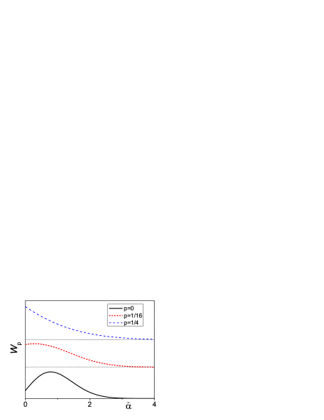
Figure 5: Evolution of distribution function at $K=2$ for different values of index $p$ (i.e. for different observation angles).

References

- (1) M. R. Andrews, C. G. Townsend, H. J. Miesner, D. S. Durfee, D. M. Kurn, and W. Ketterle, Science 275, 637 (1997).
- (2) A. Polkovnikov, E. Altman, and E. Demler, PNAS 103, 6125 (2006).
- (3) J. Schmiedmayer et al., unpublished
- (4) R. J. Glauber, Phys. Rev. Lett. , 10, 84 (1963).
- (5) Ya. M. Blanter and M. Büttiker, Phys. Rep. 336, 2 (2000).
- (6) A. Öttl, S. Ritter, M. Köhl, T. Esslinger, Phys. Rev. Lett. 95, 090404 (2005).
- (7) M. Schellekens, R. Hoppeler, A. Perrin, J. Viana Gomes, D. Boiron, A. Aspect, C. I. Westbrook, Science 310, 648 (2005).
- (8) E. Altman, E. Demler, and M. D. Lukin Phys. Rev. A 70, 013603 (2004).
- (9) M. Greiner, C. A. Regal, D. S. Jin, cond-mat/0502539.
- (10) S. Fölling, F. Gerbier, A. Widera, O. Mandel, T. Gericke, I. Bloch, Nature 434, 481 (2005).
- (11) Z. Hadzibabic, P. Kr ger, M. Cheneau, B. Battelier and J. Dalibard, preprint cond-mat/0605291, to be published in Nature.
- (12) L. S. Levitov, in ”Quantum Noise in Mesoscopic Systems”, ed. Yu. V. Nazarov (Kluwer, 2003).
- (13) W. Belzig, C. Schroll, C. Bruder, cond-mat/0412269.
- (14) C.L. Kane and M.P.A. Fisher, Phys. Rev. B 46, 15233 (1992).
- (15) P. Fendley, F. Lesage and H. Saleur, J. Stat. Phys. 85, 211 (1996).
- (16) A.O. Caldeira and A.J. Leggett, Phys. Rev. Lett. 46, 211 (1981); Physica A 121, 587 (1983).
- (17) P. DiFrancesco, P. Mathieu, D. Senechal, “Conformal Field Theory”, Springer, New York (1999).
- (18) T. Schumm, S. Hofferberth, L. M. Andersson, S. Wildermuth, S. Groth, I. Bar-Joseph, J. Schmiedmayer, P. Kr ger, Nature Physics 1, 57 (2005).
- (19) Q. Niu, I. Carusotto, A. B. Kuklov, Phys. Rev. A 73, 053604 (2006).
- (20) M. Cazalilla, J. of Phys. B: AMOP 37, S1 (2004).
- (21) We point out that Eq. (3) corresponds to periodic boundary contition. This may give a small quantitative change but will not affect the qualitative picture of the evolution of the distribution function with for long enough .
- (22) P. Fendley, F. Lesage and H. Saleur, J. of Stat. Phys. 79, 799 (1995).
- (23) V. Bazhanov, S. Lukyanov, A. Zamolodchikov, Nucl.Phys. B 549, 529 (1999).
- (24) V. V. Bazhanov, S. L. Lukyanov, A. B. Zamolodchikov, Commun. Math. Phys. 177, 381 (1996); ibid 190, 247 (1997); ibid 200, 297 (1999).
- (25) P. Dorey, R. Tateo, J. Phys. A: Math. Gen. 32, L419 (1999).
- (26) V. V. Bazhanov, S. L. Lukyanov, A. B. Zamolodchikov, J. Stat. Phys. 102, 567 (2001).
- (27) V. Gritsev, E. Altman, E. Demler, and A. Polkovnikov, in preparation.
- (28) We thank H. G. Katzgraber for pointing out to the Gumbel distribution.
- (29) E. Bertin, M. Clusel, Journal of Physics A 39, 7607 (2006).
- (30) C. M. Bender, H. F. Jones, R. J. Rivers, Phys. Lett. B 625, 333 (2005).
- (31) B. Nienhuis, Phys. Rev. Lett. 49, 1062 (1982).
- (32) J. Cardy, Ann. Phys. 318, 81 (2005).
- (33) L. N. Lipatov, Phys. Rep.; L.D. Faddeev, Korchemsky, Phys. Lett. B 342, 311 (1995); J. Ellis, N.E. Mavromatos, Eur.Phys.J. C 8, 91 (1999).
- (34) A. Stuart, J. K. Ord, Kendall’s Advanced Theory of Statistics, (New York: Oxford University Press, 1987).
- (35) R. J. Baxter, Exactly Solved Models in statistical Mechanics, Acad. Press, london (1982).
- (36) H. Friedrich and J. Trost, Phys. Rev. Lett. 76, 4869 (1996).
- (37) I. Affleck, W. Hofstetter, D. R. Nelson, U. Schollwock, J. Stat. Mech. 0410, P003 (2004).
- (38) We note that in general even purely repulsive bosons in one dimension can have effective positive scattering length and thus (see Ref. [affleck, ]).
- (39) V. Dunjko, V. Lorent, M. Olshanii, Phys. Rev. Lett. 86, 5413 (2001).