Three-body local correlation function in the Lieb-Liniger model: bosonization approach

Abstract

We develop a method for the calculation of vacuum expectation values of local operators in the Lieb-Liniger model. This method is based on a set of new identities obtained using integrability and effective theory (“bosonization”) description. We use this method to get an explicit expression for the three-body local correlation function, measured in a recent experiment [1].

1 Introduction

In this paper we present an approach to the calculation of the vacuum expectation values of local operators in the Lieb-Liniger model. Although the technique is general we shall concentrate on an particular operator, $\psi^{\dagger}(x)^{3}\psi(x)^{3},$ whose vacuum expectation value was measured in a recent experiment [1]. The physical motivation for the study of this problem and the analysis of the resulting expression has been given in Ref. [2]. Here we focus on the mathematical aspects of the problem and present the details of the derivation. In some integrable models used in condensed matter physics the exact expressions for expectation values of local operators are known, Refs. [3, 4]. However, it is not known how to use these results for the calculations in the Lieb-Liniger model.

The Lieb-Liniger model describes a one-dimensional gas of bosons interacting via a $\delta$-potential [5]. Its Hamiltonian is

$$H=\int_{0}^{L}dx\left[-\psi^{\dagger}(x)\partial_{x}^{2}\psi(x)+c\psi^{\dagger}(x)\psi^{\dagger}(x)\psi(x)\psi(x)\right],$$ (1.1)

where the units have been chosen such that $\hbar=2m=1.$ The boson fields $\psi$ and $\psi^{\dagger}$ satisfy canonical equal-time commutation relations:

$$[\psi(x),\psi^{\dagger}(y)]=\delta(x-y),\qquad[\psi^{\dagger}(x),\psi^{\dagger}(y)]=[\psi(x),\psi(y)]=0.$$ (1.2)

The system is placed on a ring of circumference $L$ and periodic boundary conditions are imposed:

$$\psi^{\dagger}(0)=\psi^{\dagger}(L),\qquad\psi(0)=\psi(L).$$ (1.3)

The particle number operator $N$ is

$$N=\int_{0}^{L}dx\,\psi^{\dagger}(x)\psi(x),$$ (1.4)

and the momentum operator $P$ is

$$P=\frac{i}{2}\int_{0}^{L}dx\left\{\left[\partial_{x}\psi^{\dagger}(x)\right]\psi(x)-\psi^{\dagger}(x)\partial_{x}\psi(x)\right\}.$$ (1.5)

These operators are integrals of motion:

$$[H,N]=[H,P]=0.$$ (1.6)

The interaction constant $c\geq 0$ has the dimension of inverse length. The dimensionless coupling strength $\gamma$ is given by

$$\gamma=\frac{c}{D},$$ (1.7)

where $D$ is the particle density,

$$D=\frac{N}{L}.$$ (1.8)

The model (1.1) has been studied extensively. Its exact eigenfunctions, spectrum, and thermodynamics were obtained during 1960s, while the calculation of its correlation functions still remains a challenge (for a review of the field see, for example, Ref. [9]). We obtain in the present paper an exact expression for the local correlation function

$$g_{3}(\gamma)=\langle\psi^{\dagger}(x)^{3}\psi(x)^{3}\rangle,$$ (1.9)

where $\langle\cdots\rangle$ denotes the expectation value in the ground state $|\mathrm{gs}\rangle$ of the system,

$$\langle\cdots\rangle\equiv\langle\mathrm{gs}|\cdots|\mathrm{gs}\rangle.$$ (1.10)

Let us formulate the main result: in the limit of the infinite number of particles taken at a finite density,

$$D\to\mathrm{const}\neq 0,\infty\qquad\text{as}\qquad N,L\to\infty,$$ (1.11)

the correlation function (1.9) is expressed as

$$\frac{g_{3}(\gamma)}{n^{3}}=\frac{3}{2\gamma}\epsilon_{4}^{\prime}-\frac{5\epsilon_{4}}{\gamma^{2}}+\left(1+\frac{\gamma}{2}\right)\epsilon_{2}^{\prime}-2\frac{\epsilon_{2}}{\gamma}-\frac{3\epsilon_{2}\epsilon_{2}^{\prime}}{\gamma}+\frac{9\epsilon_{2}^{2}}{\gamma^{2}},$$ (1.12)

where $\epsilon_{m}$ are moments of the quasi-momentum distribution function $\sigma(k)$

$$\epsilon_{m}=\left(\frac{\gamma}{\alpha}\right)^{m+1}\int_{-1}^{1}dz\,z^{m}\sigma(z),$$ (1.13)

and $\epsilon_{m}^{\prime}$ is the derivative of $\epsilon_{m}$ with respect to $\gamma.$ The function $\sigma(k)$ is the solution to the linear integral equation

$$\sigma(z)-\frac{1}{2\pi}\int_{-1}^{1}dy\,\frac{2\alpha\sigma(y)}{\alpha^{2}+(z-y)^{2}}=\frac{1}{2\pi},$$ (1.14)

where $\alpha$ is an implicit function of $\gamma:$

$$\alpha=\gamma\int_{-1}^{1}dz\,\sigma(z).$$ (1.15)

The paper is organized as follows: In section 2 we consider the $q$-boson lattice model. This is an integrable lattice model whose continuum limit is the Lieb-Liniger model. The studies of the Noether currents in the $q$-boson lattice and the Lieb-Liniger model are performed in section 3. In section 4 the $q$-boson lattice model is bosonized. In section 5 we write some contour-independent integral identities relating short- and long-distance properties of correlation functions in the $q$-boson lattice model. At long distances the results of section 4 are applicable. We thus get some non-trivial information about the short-distance properties of correlation functions. In section 6 we take the continuum limit of expressions obtained in section 5. This leads us to Eq. (1.12) for $g_{3}(\gamma).$ This equation and the contour-independent integral identities of section 5 are the main results of our paper.

2 $q$-boson lattice model

In this section a lattice regularization of the Lieb-Liniger model (1.1) is described. Lattice regularization is a natural tool to circumvent the short-range singularities discussed in section 3.2 and can, in principle, be done in many different ways. An integrable lattice regularization will be needed for our purposes. Several different regularization schemes preserving integrability are discussed in Ref. [6]. We shall use the so-called $q$-boson lattice model [7, 8] as an integrable lattice regularization of the Lieb-Liniger model. This choice is motivated by its simplicity.

In section 2.1 the $q$-boson algebra is constructed for a given lattice site. In section 2.2 we present the Hamiltonian of the $q$-boson lattice model defined on a lattice with an arbitrary number of sites, $M.$ In the continuum limit, defined by Eq. (2.19), this Hamiltonian becomes the Hamiltonian of the Lieb-Liniger model, Eq. (1.1). In section 2.3 we discuss the integrability of the $q$-boson lattice model. The generating functional of the integrals of motion is constructed using the formalism of the Quantum Inverse Scattering Method. By expanding this functional the explicit expressions for several integrals of motion are obtained. In section 2.4 we study the eigenfunctions and the eigenvalues of the integrals of motion in the $q$-boson lattice model. Finally, we apply the Hellmann-Feynman formula to one of the integrals of motion in section 2.5 with the aim of using the resulting identity in subsequent sections.

2.1 $q$-boson algebra

Consider the operators $B_{n},$ $B_{n}^{\dagger}$ and $N_{n}=N^{\dagger}_{n}$ satisfying the so-called $q$-boson algebra

$$B_{n}B_{n}^{\dagger}-q^{-2}B_{n}^{\dagger}B_{n}=1,$$ (2.1)

$$[N_{n},B_{n}]=-B_{n},\qquad[N_{n},B_{n}^{\dagger}]=B_{n}^{\dagger}.$$ (2.2)

The index $n$ labels the sites of a lattice; it will be held fixed in this section, where we work with the operators for a given lattice site. The parameter $q$ is a $c$-number and it is enough for our purposes to work with real $q\geq 1.$

Define now a Fock space for the $q$-boson algebra given by Eqs. (2.1) and (2.2). Let the basis states $|m_{j}\rangle_{j},$ $m_{j}=0,1,2,\ldots$ of the Fock space be the states of the harmonic oscillator

$$b_{n}|m_{n}\rangle_{n}=m_{n}^{1/2}|m_{n}-1\rangle_{n},\qquad b^{\dagger}_{n}|m_{n}\rangle_{n}=(m_{n}+1)^{1/2}|m_{n}+1\rangle_{n},$$ (2.3)

where $b^{\dagger}_{n}$ and $b_{n}$ are the canonically commuting creation and annihilation operators

$$[b_{n},b^{\dagger}_{n}]=1.$$ (2.4)

In this Fock space the operator $N_{n}$ entering Eqs. (2.2) acts in a manner identical with that of the operator

$$N_{n}=b^{\dagger}_{n}b_{n},$$ (2.5)

for which we have

$$N_{n}|0\rangle_{n}=0,\qquad N_{n}|m_{n}\rangle_{n}=m_{n}|m_{n}\rangle_{n},\qquad m_{n}=1,2,3,\ldots.$$ (2.6)

The operators $B^{\dagger}_{n}$ and $B_{n}$ entering Eqs. (2.1) and (2.2) act in the Fock space as follows

$$B_{n}|m_{n}\rangle_{n}=[m_{n}]_{q}^{1/2}|m_{n}-1\rangle_{n},\qquad B^{\dagger}_{n}|m_{n}\rangle_{n}=[m_{n}+1]_{q}^{1/2}|m_{n}+1\rangle_{n},$$ (2.7)

where

$$[x]_{q}\equiv\frac{1-q^{-2x}}{1-q^{-2}}.$$ (2.8)

It can be easily shown that the commutation relations (2.1) and (2.2) are consistent with Eqs. (2.6) and (2.7). Note that

$$[x]_{q}\to x\qquad\textrm{as}\qquad q\to 1,$$ (2.9)

and therefore

$$B^{\dagger}_{n}\to b^{\dagger}_{n}\qquad\textrm{and}\qquad B_{n}\to b_{n}\qquad\textrm{as}\qquad q\to 1.$$ (2.10)

It should be emphasized that the present paper deals with a representation, Eqs. (2.6) and (2.7), of the $q$-boson algebra, but not with the algebra itself. All statements concerning the $q$-boson algebra should be understood as statements about this particular representation. One can see from Eq. (2.5) that this choice of representation makes it possible to relate the operator $N_{n}$ entering Eqs. (2.2) with the canonical boson operators $b^{\dagger}_{n}$ and $b_{n}.$ It is also possible to express the operators $B^{\dagger}_{n}$ and $B_{n}$ in terms of $b^{\dagger}_{n}$ and $b_{n}:$

$$B_{n}=\sqrt{\frac{[N_{n}+1]_{q}}{N_{n}+1}}b_{n},\qquad B_{n}^{\dagger}=b^{\dagger}_{n}\sqrt{\frac{[N_{n}+1]_{q}}{N_{n}+1}}$$ (2.11)

and give an alternative form of the commutation relation (2.1):

$$[B_{n},B^{\dagger}_{n}]=q^{-2N_{n}}.$$ (2.12)

The relations (2.11) and (2.12) can be easily proven using Eqs. (2.3) and (2.7).

We see from Eqs. (2.5) and (2.11) that the relations between the $q$-boson operators $B^{\dagger}_{n}$ and $B_{n}$ and canonical boson operators $b^{\dagger}_{n}$ and $b_{n}$ are nontrivial. Furthermore, it follows from Eqs. (2.7) that

$$B_{n}^{\dagger}B_{n}|m_{n}\rangle_{n}=[m_{n}]_{q}|m_{n}\rangle_{n},$$ (2.13)

and therefore that

$$B_{n}^{\dagger}B_{n}=[N_{n}]_{q}=\frac{1-q^{-2N_{n}}}{1-q^{-2}}.$$ (2.14)

Thus, $B^{\dagger}_{n}B_{n}\neq N_{n},$ and $N_{n}$ is non-polynomial in terms of $B^{\dagger}_{n}$ and $B_{n}.$

2.2 Hamiltonian of the $q$-boson lattice model

In order to pass from the quantum mechanical (one-site) model considered in the previous section to a quantum field theory model we introduce a lattice with $M$ sites; the index $n$ in $B_{n},$ $B^{\dagger}_{n}$ and $N_{n}$ labels the lattice sites. We impose an “ultralocality” condition on the operators $B_{n_{1}},$ $B_{n_{2}}^{\dagger}$ and $N_{n_{3}}$ by requiring that they commute at different lattice sites. The basis states of the whole lattice are constructed as the tensor product of the local basis states:

$$|0\rangle=\otimes_{j=1}^{M}|0\rangle_{j},\qquad|m\rangle=\otimes_{j=1}^{M}|m_{j}\rangle_{j}.$$ (2.15)

The Hamiltonian for the $q$-boson lattice model is defined as follows:

$$H_{q}=-\frac{1}{\delta^{2}}\sum_{n=1}^{M}(B_{n}^{\dagger}B_{n+1}+B_{n+1}^{\dagger}B_{n}-2N_{n})$$ (2.16)

with the periodic boundary conditions $M+1=1$ imposed. Here $\delta$ is the lattice spacing. The factor $\delta^{-2}$ is introduced to ensure the proper continuum limit. One can check using the $q$-boson algebra, Eqs. (2.1) and (2.2), that $H_{q}$ commutes with the number operator

$$N=\sum_{n=1}^{M}N_{n}.$$ (2.17)

Since $N$ is non-polynomial in terms of $B^{\dagger}_{n}$ and $B_{n},$ which can be seen from Eq. (2.14), $H_{q}$ is non-polynomial in terms of these fields. It is non-polynomial in terms of the canonical lattice bosons $b^{\dagger}_{n}$ and $b_{n}$ as well, now due to the non-polynomiality of the hopping term. Thus the model is interacting and the interaction is encoded in the deformation parameter $q:$ if one takes $q\to 1$ the result will be a quadratic boson Hamiltonian on a lattice, describing nearest-neighbor hopping:

$$H_{q}\to-\frac{1}{\delta^{2}}\sum_{n=1}^{M}(b^{\dagger}_{n}b_{n+1}+b^{\dagger}_{n+1}b_{n}-2N_{n})\qquad\text{as}\qquad q\to 1.$$ (2.18)

The limit $q\to 1$ is somehow trivial. It is much more fruitful to consider the following limit: let $\delta\to 0,$ $M\to\infty,$ and $q\to 1,$ while $L$ and $c$ are kept constant:

$$L=M\delta,\qquad c/2=\kappa\delta^{-1},\qquad\text{as}\qquad\delta\to 0,\qquad M\to\infty,\qquad\kappa\to 0,$$ (2.19)

where $\kappa$ is related to $q$ as follows

$$q=e^{\kappa}.$$ (2.20)

The limit (2.19) will be called the continuum limit of the $q$-boson lattice model. The sums in the continuum limit are converted into integrals in the usual way

$$\delta\sum_{n=1}^{M}\to\int_{0}^{L}dx.$$ (2.21)

For any $q$-deformed quantity $[x]_{q}$, Eq. (2.8), the following expansion is valid

$$[x]_{q}=x-\kappa x(x-1)+\frac{\kappa^{2}}{3}x(x-1)(2x-1)+\dots,\qquad\kappa\to 0,$$ (2.22)

where $q$ is related to $\kappa$ by Eq. (2.20). Therefore

$$\sqrt{\frac{[N_{n}+1]_{q}}{N_{n}+1}}=1-\frac{\kappa}{2}N_{n}+\frac{\kappa^{2}}{24}N_{n}(5N_{n}+4)+\dots,\qquad\kappa\to 0.$$ (2.23)

We define the continuum boson fields $\psi(x)$ and $\psi^{\dagger}(x)$ by

$$\psi^{\dagger}(x)=\delta^{-1/2}b^{\dagger}_{n},\qquad\psi(x)=\delta^{-1/2}b_{n},$$ (2.24)

where

$$x=\delta n.$$ (2.25)

The fields $\psi^{\dagger}(x)$ and $\psi(x)$ satisfy canonical commutation relations (1.2). One can easily check that the $q$-boson Hamiltonian (2.16) becomes the Hamiltonian of the Lieb-Liniger model (1.1) in the continuum limit (2.19).

Finally, we discuss the number of particles and momentum operators in the $q$-boson lattice model and their continuum limit. We have defined the number operator in the $q$-boson lattice model by Eq. (2.17). The continuum limit (2.19) of this operator is given by Eq. (1.4). The momentum operator is defined in the $q$-boson lattice model as follows:

$$P_{q}=-\frac{i}{2}\frac{1}{\delta}\sum_{n=1}^{M}(B^{\dagger}_{n}B_{n+1}-B^{\dagger}_{n+1}B_{n}).$$ (2.26)

Its continuum limit is given by Eq. (1.5). To avoid any confusion, we note that $P_{q}$ is not a generator of lattice translations, that is

$$e^{-iP_{q}}B_{n}e^{iP_{q}}\neq B_{n+1}.$$ (2.27)

However, its continuum limit (1.5) is such a generator for the continuum model:

$$e^{-iaP}\psi(x)e^{iaP}=\psi(x+a).$$ (2.28)

It is due to the property (2.28) that we call $P_{q}$ the momentum operator. We shall not need to know an explicit form of the true momentum operator $P^{\mathrm{true}}_{q}$ which generates the lattice translations in the $q$-boson lattice model.

2.3 Integrals of motion in the $q$-boson lattice model

An infinite set of integrals of motion in the $q$-boson lattice model can be constructed using the Quantum Inverse Scattering Method. A detailed description of this method is given, for example, in Ref. [9], and it was applied to the $q$-boson lattice model, in particular, in Refs. [7, 8]. We give in the present section a schematic description of the method, referring the reader to the Refs. [7, 8, 9] for details. The main purpose of the section is to obtain Eqs. (2.44)–(2.47).

The so-called $L$-operator for the $q$-boson lattice model is defined by

$$L_{n}(\lambda)=\left(\begin{array}[]{cc}e^{\lambda}&\chi B_{n}^{\dagger}\\ \chi B_{n}&e^{-\lambda}\end{array}\right),$$ (2.29)

where

$$\chi=\sqrt{1-q^{-2}}=\sqrt{1-e^{-2\kappa}}.$$ (2.30)

The $L$-operator (2.29) is a $2\times 2$ matrix with the entries being quantum operators acting in the infinite-dimensional Fock space defined by Eq. (2.3). The Quantum Inverse Scattering Method is based on the existence of the intertwining relation for the $L$-operator:

$$R(\lambda,\mu)\left(L_{n}(\lambda)\otimes L_{n}(\mu)\right)=\left(L_{n}(\mu)\otimes L_{n}(\lambda)\right)R(\lambda,\mu)$$ (2.31)

with the $R$-matrix defined by

$$R(\lambda,\mu)=\left(\begin{array}[]{cccc}f(\mu,\lambda)&0&0&0\\ 0&g(\mu,\lambda)&q&0\\ 0&q^{-1}&g(\mu,\lambda)&0\\ 0&0&0&f(\mu,\lambda)\end{array}\right),$$ (2.32)

where

$$f(\lambda,\mu)=\frac{\sinh(\lambda-\mu+\kappa)}{\sinh(\lambda-\mu)},\qquad g(\lambda,\mu)=\frac{\sinh(\kappa)}{\sinh(\lambda-\mu)}.$$ (2.33)

Recall that the tensor product for $2\times 2$ matrices $a$ and $b$ is defined as follows:

$$a\otimes b=\left(\begin{array}[]{cc}a_{11}&a_{12}\\ a_{21}&a_{22}\end{array}\right)\otimes\left(\begin{array}[]{cc}b_{11}&b_{12}\\ b_{21}&b_{22}\end{array}\right)=\left(\begin{array}[]{cccc}a_{11}b_{11}&a_{11}b_{12}&a_{12}b_{11}&a_{12}b_{12}\\ a_{11}b_{21}&a_{11}b_{22}&a_{12}b_{21}&a_{12}b_{22}\\ a_{21}b_{11}&a_{21}b_{12}&a_{22}b_{11}&a_{22}b_{12}\\ a_{21}b_{21}&a_{21}b_{22}&a_{22}b_{21}&a_{22}b_{22}\end{array}\right).$$ (2.34)

The monodromy matrix $T(\lambda)$ is defined as a matrix product of the $L$-operators taken over all lattice sites

$$T(\lambda)=\left(\begin{array}[]{cc}A(\lambda)&B(\lambda)\\ C(\lambda)&D(\lambda)\end{array}\right)=L_{M}(\lambda)L_{M-1}(\lambda)\cdots L_{1}(\lambda).$$ (2.35)

The entries $A(\lambda),\ldots,D(\lambda)$ of the monodromy matrix are quantum operators acting in the tensor product of the local Fock spaces over all sites of the lattice. Due to the relation (2.31) and the commutativity of the entries of the $L$-operator (2.29) at different lattice sites one has the intertwining relation for the monodromy matrix

$$R(\lambda,\mu)\left(T(\lambda)\otimes T(\mu)\right)=\left(T(\mu)\otimes T(\lambda)\right)R(\lambda,\mu).$$ (2.36)

Equation (2.36) defines $16$ commutation relations for the operators entering the monodromy matrix. We write explicitly those relations which we shall use in deriving the Bethe equations in section 2.4:

$$qA(\lambda)B(\mu)=f(\lambda,\mu)B(\mu)A(\lambda)+g(\mu,\lambda)B(\lambda)A(\mu),$$ (2.37)

$$qD(\lambda)B(\mu)=f(\mu,\lambda)B(\mu)D(\lambda)+g(\lambda,\mu)B(\lambda)D(\mu),$$ (2.38)

$$[B(\lambda),B(\mu)]=0.$$ (2.39)

The transfer matrix $\tau(\lambda)$ is defined as the trace over the matrix space of the monodromy matrix

$$\tau(\lambda)=\mathrm{Tr}\,T(\lambda)=A(\lambda)+D(\lambda).$$ (2.40)

It can be proven (see chapter VI of Ref. [9] for details) that for any $\lambda$ and $\mu$

$$[\tau(\lambda),\tau(\mu)]=0$$ (2.41)

which implies that $\tau$ is a generating function of the integrals-of-motion of the problem: expanding $\tau(\lambda)$ in $\lambda$ one gets a set of commuting integrals-of-motion $I_{m}$. This set can be chosen in many different ways since any analytic function of $\tau(\lambda)$ can play the role of the generating functional. We, however, impose an additional very restrictive locality condition on these integrals by requiring them to be written in the following form

$$I_{m}=\delta\sum_{n=1}^{M}\mathcal{J}^{(m)}_{\tau}(n),$$ (2.42)

where the operators $\mathcal{J}^{(m)}_{\tau}(n)$ act nontrivially in $m$ neighboring lattice sites only. The subscript $\tau$ appears in $\mathcal{J}^{(m)}_{\tau}(n)$ since these local operators are $\tau$-components of the corresponding Noether currents, which will be discussed in section 3. To get the set $\{I_{m}\}$ we introduce the variable

$$\zeta=e^{\lambda}$$ (2.43)

and consider the expression

$$I_{m}=\left.\frac{1}{(2m)!}\frac{d^{2m}}{d\zeta^{2m}}\ln\left[\zeta^{M}\tau(\zeta)\right]\right|_{\zeta\to 0},\qquad m=1,2,3,\ldots.$$ (2.44)

We assume that $\lambda$ is real, therefore $\zeta$ is real and nonnegative. The local operators $\mathcal{J}_{\tau}^{(1)}(n),$ $\mathcal{J}_{\tau}^{(2)}(n)$ and $\mathcal{J}_{\tau}^{(3)}(n)$ are

$$\mathcal{J}_{\tau}^{(1)}(n)=\frac{1}{\delta}\chi^{2}B^{\dagger}_{n}B_{n+1}$$ (2.45)

$$\mathcal{J}_{\tau}^{(2)}(n)=\frac{1}{\delta}\chi^{2}\left(1-\frac{\chi^{2}}{2}\right)\left(B^{\dagger}_{n}B_{n+2}-\frac{\chi^{2}}{2-\chi^{2}}B_{n}^{\dagger}B_{n}^{\dagger}B_{n+1}B_{n+1}-\chi^{2}B_{n}^{\dagger}B_{n+1}^{\dagger}B_{n+1}B_{n+2}\right)$$ (2.46)

and

$$\mathcal{J}_{\tau}^{(3)}(n)=\frac{1}{\delta}\chi^{2}\left(1-\chi^{2}+\frac{\chi^{4}}{3}\right)\left(\vphantom{\frac{\chi^{4}}{3}}B^{\dagger}_{n}B_{n+3}-\chi^{2}B^{\dagger}_{n}B^{\dagger}_{n}B_{n+1}B_{n+2}-\chi^{2}B^{\dagger}_{n}B^{\dagger}_{n+1}B_{n+1}B_{n+3}\right.\\ -\chi^{2}B^{\dagger}_{n}B^{\dagger}_{n+1}B_{n+2}B_{n+2}-\chi^{2}B^{\dagger}_{n}B^{\dagger}_{n+2}B_{n+2}B_{n+3}+\frac{\chi^{4}}{3-3\chi^{2}+\chi^{4}}B^{\dagger}_{n}B^{\dagger}_{n}B^{\dagger}_{n}B_{n+1}B_{n+1}B_{n+1}\\ +\chi^{4}B^{\dagger}_{n}B^{\dagger}_{n}B^{\dagger}_{n+1}B_{n+1}B_{n+1}B_{n+2}+\chi^{4}B^{\dagger}_{n}B^{\dagger}_{n+1}B^{\dagger}_{n+1}B_{n+1}B_{n+2}B_{n+2}\\ +\left.\chi^{4}B^{\dagger}_{n}B^{\dagger}_{n+1}B^{\dagger}_{n+2}B_{n+1}B_{n+2}B_{n+3}\vphantom{\frac{\chi^{4}}{3}}\right)$$ (2.47)

respectively. To calculate $g_{3}(\gamma),$ Eq. (1.9), we will need $\mathcal{J}_{\tau}^{(1)}$ and $\mathcal{J}_{\tau}^{(2)}$; the explicit expression for $\mathcal{J}_{\tau}^{(3)}$ is displayed in order to illustrate how the complexity of $\mathcal{J}_{\tau}^{(m)}$ grows with increasing $m$.

The integrals $I_{m}$ are non-Hermitian, they contain both real and imaginary part. Using the involution

$$[\tau(\zeta)]^{\dagger}=\tau(\zeta^{-1})$$ (2.48)

it may be shown that

$$[I^{\dagger}_{m},I_{n}]=0\qquad\text{for any}\quad m,n.$$ (2.49)

For the integrals of motion $I^{\dagger}_{m},$ we use the following notation

$$I_{-m}\equiv I^{\dagger}_{m},\qquad m=1,2,3,\ldots,$$ (2.50)

and for the local operators $\mathcal{J}_{\tau}$

$$\mathcal{J}^{(-m)}_{\tau}(n)\equiv[\mathcal{J}^{(m)}_{\tau}(n)]^{\dagger},\qquad m=1,2,3,\dots.$$ (2.51)

Using the involution (2.48) one gets for $I_{-m}$

$$I_{-m}=\left.\frac{1}{(2m)!}\frac{d^{2m}}{d\zeta^{2m}}\ln\left[\zeta^{M}\tau(\zeta^{-1})\right]\right|_{\zeta\to 0},\qquad m=1,2,3,\ldots.$$ (2.52)

A set of common eigenfunctions of $I_{m},$ $m=\pm 1,\pm 2,\dots$ is constructed in section 2.4.

The local operators $\mathcal{J}_{\tau}^{(m)}(n)$ generated by Eqs. (2.42) and (2.44) are polynomial in $B^{\dagger}_{n}$ and $B_{n},$ while the one-site number operator $N_{n}$ is non-polynomial in these variables, as was noticed below Eq. (2.14). Therefore, the number operator $N,$ Eq. (2.17), cannot be expressed as a finite linear combination of the integrals of motion $I_{m},$ Eq. (2.44). It is, however, clear from the structure of $\mathcal{J}_{\tau}^{(m)}(n)$ that

$$[N,\mathcal{J}_{\tau}^{(m)}(n)]=0,\qquad m=\pm 1,\pm 2,\dots.$$ (2.53)

Indeed, $N$ commutes with any monomial containing an equal number of the creation and annihilation operators, $B^{\dagger}$ and $B.$ It follows from Eq. (2.53) that

$$[N,I_{m}]=0,\qquad m=\pm 1,\pm 2,\dots.$$ (2.54)

To stress that $N$ is one of the integrals of motion, we shall use the following notation

$$N\equiv I_{0},\qquad\mathcal{J}_{\tau}^{(0)}(n)\equiv\frac{1}{\delta}N_{n}.$$ (2.55)

The Hamiltonian (2.16) can thus be written as

$$H_{q}=-\frac{1}{\chi^{2}\delta^{2}}(I_{1}+I_{-1}-2\chi^{2}I_{0}),$$ (2.56)

and the momentum operator (2.26) as

$$P_{q}=-\frac{i}{2}\frac{1}{\chi^{2}\delta}(I_{1}-I_{-1}).$$ (2.57)

2.4 Eigenfunctions and eigenvalues of the integrals of motion in the $q$-boson lattice model

We have constructed in section 2.3 a set of integrals of motion $I_{m},$ Eq. (2.44), of the $q$-boson lattice model on a lattice with an arbitrary number of sites, $M$. We find in the present section their common eigenfunctions and their eigenvalues using the Algebraic Bethe Ansatz technique [9], an important ingredient of the Quantum Inverse Scattering Method. The eigenvalues of all $I_{m}$ are defined in the $N$-particle sector by $N$ parameters called quasi-momenta. These quasi-momenta are the solutions of the system of nonlinear equations called the Bethe equations. Following the presentation of Ref. [9], Chap. I, we find from the analysis of the Bethe equations the ground state quasi-momentum distribution and study its properties in the limit defined by Eq. (2.80).

The cornerstone of the Algebraic Bethe Ansatz method is the fact that the vacuum $|0\rangle$ defined by Eq. (2.15) annihilates the $C(\lambda)$ entry of the monodromy matrix (2.35) and is an eigenfunction for the $A(\lambda)$ and $D(\lambda)$ entries:

$$A(\lambda)|0\rangle=e^{M\lambda}|0\rangle,\qquad D(\lambda)|0\rangle=e^{-M\lambda}|0\rangle.$$ (2.58)

Since $N$ is a good quantum number, one can work in the $N$-particle sector. Define a set of states by the following formula

$$|\psi_{N}(\lambda_{1},\ldots,\lambda_{N})\rangle=\prod_{j=1}^{N}B(\lambda_{j})|0\rangle.$$ (2.59)

These states (often called the Bethe states) are eigenfunctions of the transfer matrix (2.40) and, hence, of the integrals of motion $I_{m},$ $m=\pm 1,\pm 2,\dots,$ if the parameters $\lambda_{1},\ldots,\lambda_{M}$ satisfy a system of coupled nonlinear equations (called the Bethe equations),

$$e^{2M\lambda_{j}}=\prod_{\genfrac{}{}{0.0pt}{1}{k=1}{k\neq j}}^{N}\frac{f(\lambda_{k},\lambda_{j})}{f(\lambda_{j},\lambda_{k})},\qquad j=1,\ldots,N.$$ (2.60)

The eigenvalues $\theta_{N}$ of the transfer matrix acting on the Bethe states (2.59) are given by

$$\tau(\lambda)|\psi_{N}\rangle=\theta_{N}(\lambda,\{\lambda_{j}\})|\psi_{N}\rangle,$$ (2.61)

$$q^{N}\theta_{N}(\lambda,\{\lambda_{j}\})=e^{M\lambda}\prod_{j=1}^{N}f(\lambda,\lambda_{j})+e^{-M\lambda}\prod_{j=1}^{N}f(\lambda_{j},\lambda).$$ (2.62)

The eigenvalues of the integrals of motion $I_{m},$ $m=\pm 1,\pm 2,\dots$ acting on the Bethe states (2.59) can be obtained by acting with the representations (2.44) and (2.52) onto $|\psi_{N}\rangle$ and using Eqs. (2.43), (2.61) and (2.62). The calculations are tedious, while the final result is surprisingly simple:

$$I_{m}|\psi_{N}\rangle=\left(1-q^{-2|m|}\right)\frac{1}{|m|}\sum_{j=1}^{N}e^{-2m\lambda_{j}}|\psi_{N}\rangle,\qquad m=\pm 1,\pm 2,\dots.$$ (2.63)

It is useful to mention that, in order to calculate the correlation function (1.9) we shall need to know the spectrum of the integrals $I_{\pm 1}$ and $I_{\pm 2}$ only. For $|m|>2$ we did not obtain Eq. (2.63) analytically. Instead, we simply checked that it is correct for some given values of $N,$ $M$ and $m$ using the Mathematica package.

It will be convenient to use instead of $\lambda_{1},\ldots,\lambda_{N}$ a set of quasi-momenta $p_{1},\ldots,p_{N}:$

$$\lambda_{j}=i\frac{p_{j}}{2},\qquad j=1,\ldots,N.$$ (2.64)

Written in these variables, the Bethe equations (2.60) are

$$e^{iMp_{j}}=\prod_{\genfrac{}{}{0.0pt}{1}{k=1}{k\neq j}}^{N}\frac{\sin[\frac{1}{2}(p_{j}-p_{k})+i\kappa]}{\sin[\frac{1}{2}(p_{j}-p_{k})-i\kappa]},\qquad j=1,\ldots,N.$$ (2.65)

Using Eqs. (2.56), (2.63) and (2.64), one gets for the eigenvalues of the Hamiltonian (2.16):

$$E_{N}=\frac{4}{\delta^{2}}\sum_{j=1}^{N}\sin^{2}\frac{p_{j}}{2}.$$ (2.66)

We now discuss some properties of the Bethe equations necessary to identify the ground state of the model and to take the limit (2.80). The analysis will be very similar to that one carried out for the Lieb-Liniger model in Ref. [9], Chap. I, so we omit several long proofs, referring the reader to Ref. [9] for details.

(i) All the solutions $p_{j}$ of the Bethe equations (2.65) are real. The proof is the same as that given for the Lieb-Liniger model in Ref. [9], page 11.

(ii) It follows from Eq. (2.66) that $E_{N}$ is a periodic function of the quasi-momenta $p_{j}$ with period $2\pi.$ We shall work with quasi-momenta lying in the interval

$$-\pi<p_{j}<\pi,\qquad j=1,\ldots,N.$$ (2.67)

The condition (2.67) will be assumed in all subsequent formulas.

(iii) We write the Bethe equations (2.65) in the logarithmic form

$$Mp_{j}+\sum_{k=1}^{N}\theta(p_{j}-p_{k})=2\pi\left(n_{j}+\frac{N-1}{2}\right),\qquad j=1,\ldots,N,$$ (2.68)

where the parameters $n_{j}$ take arbitrary integer values:

$$n_{j}\text{ is an arbitrary integer},\qquad j=1,\dots,N.$$ (2.69)

From now on we shall work with odd $N:$

$$N\text{ is odd}.$$ (2.70)

The function $\theta(p)$ is

$$\theta(p)=i\ln\frac{\sin\left(i\kappa+\frac{1}{2}p\right)}{\sin\left(i\kappa-\frac{1}{2}p\right)},\qquad\theta(-p)=-\theta(p).$$ (2.71)

The derivative of $\theta(p)$ is positive,

$$\theta^{\prime}(p)=\frac{i\sin(2i\kappa)}{2\sin(i\kappa+\frac{1}{2}p)\sin(i\kappa-\frac{1}{2}p)}=\frac{\sinh(2\kappa)}{\cosh(2\kappa)-\cos p}>0,$$ (2.72)

therefore $\theta(p)$ grows monotonously in the interval $-\pi<p<\pi$ (recall that the condition (2.67) is assumed).

(iv) For any set $\{n_{j}\},$ Eq. (2.69), there exists a uniquely defined set $\{p_{j}\}$ of solutions of the Bethe equations (2.68). The proof is the same as that given for the Lieb-Liniger model in Ref. [9], page 12.

(v) We write, using Eq. (2.68),

$$M(p_{j}-p_{s})+\sum_{k=1}^{N}\left[\theta(p_{j}-p_{k})-\theta(p_{s}-p_{k})\right]=2\pi(n_{j}-n_{s}),\qquad j,s=1,\ldots,N.$$ (2.73)

Since $\theta^{\prime}(p)>0,$ Eq. (2.72), the left hand side of the Eq. (2.73) is a monotonically growing function of the parameter $p_{j}-p_{k}.$ Therefore, if $n_{j}>n_{s}$ then $p_{j}>p_{s};$ if $n_{j}=n_{s}$ then $p_{j}=p_{s}.$ We have thus shown that the set of quasi-momenta $\{p_{j}\}$ is uniquely characterized by the set $\{n_{j}\},$ and vice versa.

(vi) Like for the Lieb-Liniger model (Ref. [9], page 14) the energy functional (2.66) taken on the sets $\{p_{j}\}$ of the solutions of the Bethe equations has the minimum in the sector with the fixed number of particles, $N,$ if $n_{j}$ take the values

$$n_{j}=-N+j,\qquad j=1,\ldots,N.$$ (2.74)

The Bethe equations (2.68) for the ground state are, therefore,

$$Mp_{j}+\sum_{k=1}^{N}\theta(p_{j}-p_{k})=2\pi\left(j-1-\frac{N-1}{2}\right),\qquad j=1,\ldots,N.$$ (2.75)

The ground state is obviously non-degenerate.

(vii) It is obvious that the set $\{p_{j}\}$ of the solutions of Eq. (2.75) is symmetric with respect to zero. It follows then from Eqs. (2.63) and (2.64) that the eigenvalues of $I_{m},$ $m=\pm 1,\pm 2,\dots$ corresponding to the ground state wave function $|\mathrm{gs}\rangle$ are real, and

$$\langle I_{m}\rangle=\langle I_{-m}\rangle,\qquad m=1,2,3,\dots$$ (2.76)

where $I_{-m}$ is defined by Eq. (2.50).

(viii) The ground state wave function is translationally invariant. This implies that the ground state average $\langle\mathcal{J}_{\tau}^{(m)}(n)\rangle$ is $n$-independent. Using this property, one gets from Eq. (2.42)

$$\langle I_{m}\rangle=\delta M\langle\mathcal{J}_{\tau}^{(m)}\rangle.$$ (2.77)

Comparing this with Eq. (2.76), one arrives at

$$\langle\mathcal{J}^{(-m)}_{\tau}\rangle=\langle\mathcal{J}^{(m)}_{\tau}\rangle,$$ (2.78)

where $\mathcal{J}_{\tau}^{(-m)}$ is defined by Eq. (2.51). We recall that the size of the system, $L,$ is the product of the number of the sites, $M,$ and the lattice spacing, $\delta,$ Eq. (2.19), therefore the particle density, Eq. (1.8), can be written as follows

$$D=\frac{\langle I_{0}\rangle}{L}=\langle\mathcal{J}_{\tau}^{(0)}\rangle.$$ (2.79)

We are interested in the ground-state properties of the $q$-boson lattice model in the limit

$$N\to\infty,\qquad M\to\infty.$$ (2.80)

We introduce the quasi-momentum distribution function $\rho(p_{j})$ by means of the following identity

$$\sum_{j=1}^{N}=M\sum_{j=1}^{N}\rho(p_{j})(p_{j+1}-p_{j}),$$ (2.81)

where

$$\rho(p_{j})=\frac{1}{M(p_{j+1}-p_{j})}.$$ (2.82)

The quasi-momenta $p_{j}$ fill the symmetric interval $-\Lambda\leq p_{j}\leq\Lambda$ and one has $p_{j+1}-p_{j}\sim M^{-1}$ (Ref. [9], page 14). For an arbitrary function $f(p_{j})$ one has

$$\sum_{j=1}^{N}f(p_{j})\to M\int_{-\Lambda}^{\Lambda}dp\,\rho(p)f(p).$$ (2.83)

The parameter $\Lambda$ plays a role analogous to that of the Fermi momentum: all states with $|p|<\Lambda$ are occupied, and all states with $|p|>\Lambda$ are empty. The value of $\Lambda$ is defined by the normalization condition

$$\frac{N}{M}=\int_{-\Lambda}^{\Lambda}dp\,\rho(p).$$ (2.84)

The Bethe equations (2.75) become in the limit (2.80) a linear integral equation for the ground state quasi-momentum distribution $\rho(p)$

$$\rho(p)-\frac{1}{2\pi}\int_{-\Lambda}^{\Lambda}d\tilde{p}\,K(p-\tilde{p})\rho(\tilde{p})=\frac{1}{2\pi},$$ (2.85)

with the kernel $K(p)$ given by Eq. (2.72),

$$K(p)=\theta^{\prime}(p)=\frac{\sinh(2\kappa)}{\cosh(2\kappa)-\cos p}.$$ (2.86)

Equation (2.85) is often called the Lieb equation.

Having defined $\rho(p)$ and $\Lambda$ one can easily get the ground-state expectation values of the integrals of motion, $\langle I_{m}\rangle,$ in the limit (2.80). In particular,

$$\frac{\langle I_{1}\rangle}{M}=\chi^{2}\int_{-\Lambda}^{\Lambda}dp\,\rho(p)\cos p,$$ (2.87)

and

$$\frac{\langle I_{2}\rangle}{M}=\chi^{2}\left(1-\frac{\chi^{2}}{2}\right)\int_{-\Lambda}^{\Lambda}dp\,\rho(p)\cos 2p.$$ (2.88)

The ground-state energy of the system can be obtained from Eq. (2.56) or (2.66):

$$\frac{E_{N}}{M}=\frac{\langle H_{q}\rangle}{M}=\frac{4}{\delta^{2}}\int_{-\Lambda}^{\Lambda}dp\,\rho(p)\sin^{2}\frac{p}{2}.$$ (2.89)

We shall make use of the properties of $\langle I_{m}\rangle$ in section 6.1.

2.5 Hellmann-Feynman theorem

In this section we use the Hellmann-Feynman theorem to derive an identity for the ground-state average of some local operator in the $q$-boson lattice model. This identity is given by Eqs. (2.92) and (2.96) below, and will be used in section 6.2.

It was shown in section 2.4 that the eigenfunctions (2.59) of the $q$-boson Hamiltonian (2.16) are the eigenfunctions for the integrals of motion Eq. (2.44) and their Hermitian conjugate Eq. (2.50). Since $I_{1}|\mathrm{gs}\rangle=I_{1}^{\dagger}|\mathrm{gs}\rangle,$ Eq. (2.76), one has

$$\frac{d}{dq}\langle I_{1}\rangle=\left\langle\frac{d}{dq}I_{1}\right\rangle.$$ (2.90)

where $\langle\cdots\rangle$ denotes the ground state average and $q$ is the deformation parameter defined by Eq. (2.1). Equation (2.90) is known under the name of the Hellmann-Feynman theorem. The explicit expression for $I_{1}$ via local fields $B_{n}^{\dagger}$ and $B_{n}$ is given by Eqs. (2.42) and (2.45). Using the translational invariance of the ground state, implying that

$$\langle B^{\dagger}_{j_{1}}\dots B_{j_{m}}\rangle=\langle B^{\dagger}_{j_{1}+k}\dots B_{j_{m}+k}\rangle$$ (2.91)

where $k$ is an arbitrary integer, equation (2.90) can be written as follows:

$$\frac{d}{dq}\langle\chi^{-2}I_{1}\rangle=M\left\langle\frac{d}{dq}(B^{\dagger}_{j}B_{j+1})\right\rangle.$$ (2.92)

The dependence of the operators $B_{j}$ and $B^{\dagger}_{j}$ on the parameter $q$ can be analyzed using the representation (2.11). One gets from this representation

$$\frac{d}{dq}B_{j}=[N_{j}+1]^{-1/2}_{q}\frac{d}{dq}[N_{j}+1]^{1/2}_{q}B_{j},$$ (2.93)

$$\frac{d}{dq}B_{j}^{\dagger}=B_{j}^{\dagger}[N_{j}+1]^{-1/2}_{q}\frac{d}{dq}[N_{j}+1]^{1/2}_{q}.$$ (2.94)

Introducing the notation

$$g(q,x)=[x+1]_{q}^{-1/2}\frac{d}{dq}[x+1]_{q}^{1/2}=\frac{1}{q}\left(\frac{x+1}{q^{2x+2}-1}-\frac{1}{q^{2}-1}\right)$$ (2.95)

and combining Eqs. (2.93) and (2.94) one finds

$$\frac{d}{dq}(B^{\dagger}_{j}B_{j+1})=B^{\dagger}_{j}g(q,N_{j})B_{j+1}+B^{\dagger}_{j}g(q,N_{j+1})B_{j+1}.$$ (2.96)

3 Noether currents

Noether’s theorem is an important ingredient of Quantum Field Theory. In short, it states that symmetries imply conservation laws. More precisely, if the action of a system is invariant under an infinitesimal transformation of the fields, then there exists a function of these fields whose divergence is zero. This function is called the Noether current associated with the symmetry. One can say more about this function if the symmetry transformation leaves the Lagrangian (or, even better, the Lagrangian density) and not just the action invariant [10].

For integrable models, however, it is often more natural to work within the Hamiltonian formalism rather than within the Lagrangian one. This is due to the fact that explicit expressions for the integrals of motion are usually known in these models. In case of the $q$-boson lattice model the local integrals of motion are generated by Eq. (2.44) and explicit expressions for $\mathcal{J}_{\tau}^{(m)},$ like (2.45)–(2.47), can be, in principle, written down up to an arbitrarily large $m.$ The operator $\mathcal{J}_{\tau}^{(m)}$ can be recognized as the imaginary-time component of the conserved current $\mathcal{J}^{(m)}.$ By calculating the commutator of $\mathcal{J}_{\tau}^{(m)}$ with the Hamiltonian one gets the space component $\mathcal{J}_{x}^{(m)}$ of the corresponding conserved current. The continuity equation for $\mathcal{J}^{(m)}$ will be extensively used further derivations.

In section 3.1 we recall briefly the notion of the Noether currents in the Hamiltonian formalism. Noether currents in the Lieb-Liniger model are considered in section 3.2. We demonstrate the problem of making an unambiguous definition of higher integrals of motion in this model. It is because of this problem that we are working with the $q$-boson lattice regularization (described in section 2) of the Lieb-Liniger model. Noether currents in the $q$-boson lattice model are considered in section 3.3. Finally, in section 3.4 we subject the $q$-boson lattice model to a local gauge transformation and study the behavior of the Noether currents under this transformation.

3.1 Noether currents in the Hamiltonian formalism

To begin with, let us introduce some notation. It is often more convenient in Quantum Field Theory to work with the Euclidean (imaginary) time $\tau$ rather than with the Minkowski time $t:$

$$\tau=it.$$ (3.1)

We denote by $g_{\mu\nu}$ the metric tensor for two-dimensional space-time theories:

$$g_{\mu\nu}=\left\{\begin{array}[]{ll}\mathrm{diag}(1,-1)&\qquad\text{Minkowski}\\ \mathrm{diag}(1,1)&\qquad\text{Euclidean}\end{array}\right.$$ (3.2)

The summation is performed over the contracted indices,

$$a_{\mu}b^{\mu}\equiv\sum_{\mu}a_{\mu}b^{\mu}$$ (3.3)

and the rules for converting between covariant and contravariant indices are

$$a_{\mu}=g_{\mu\nu}a^{\nu},\qquad a^{\mu}=g^{\mu\nu}a_{\nu},\qquad g_{\mu\nu}g^{\nu\sigma}=\delta_{\mu}^{\sigma}.$$ (3.4)

The Hamiltonian $H$ of a theory can be defined as the generator of time-translations for an arbitrary operator $\mathcal{O}:$

$$\mathcal{O}(x,t)=e^{itH}\mathcal{O}(x,0)e^{-itH}.$$ (3.5)

We assume that the Hamiltonian is time-independent:

$$\frac{\partial H}{\partial t}=\frac{dH}{dt}=0.$$ (3.6)

Then the equation of motion for $\mathcal{O}(x,t)$ following from Eq. (3.5) is

$$\frac{\partial}{\partial t}\mathcal{O}_{M}(x,t)=\frac{d}{dt}\mathcal{O}_{M}(x,t)=i[H,\mathcal{O}_{M}(x,t)].$$ (3.7)

We note that all the dependence on $t$ of the operator $\mathcal{O}_{M}(x,t)$ is explicitly given by the evolution operator $e^{itH},$ Eq. (3.5), and there is no need to distinguish the partial $\partial/\partial t$ and full $d/dt$ derivatives. The subscript $M$ is used in Eq. (3.7) to indicate that it is written in the Minkowski time $t.$ Written in the Euclidean time $\tau,$ Eq. (3.1), the equation of motion (3.7) takes the form

$$\frac{\partial}{\partial\tau}\mathcal{O}_{E}(x,\tau)=\frac{d}{d\tau}\mathcal{O}_{E}(x,\tau)=[H,\mathcal{O}_{E}(x,\tau)],$$ (3.8)

where $\mathcal{O}_{E}(x,\tau)=\mathcal{O}_{M}(x,t).$ We will mainly work with the Euclidean time and therefore we drop the subscript $E$ to shorten notation. We shall also drop one or both of the arguments $x,\tau$ in $\mathcal{O}(x,\tau)$ when they can be recovered from the context.

Impose a locality condition onto the operator $\mathcal{O}(x):$ suppose that this operator, taken at a point $x,$ depends on the basis fields $\psi$ and $\psi^{\dagger}$ (and their derivatives) taken at this point exclusively. Equations (3.13) and (3.16) provide us with examples of the operators of such type. If, in addition, $\int_{0}^{L}dx\,\mathcal{O}(x)$ is an integral of motion,

$$[H,\int_{0}^{L}dx\,\mathcal{O}(x)]=0,$$ (3.9)

then

$$[H,\mathcal{O}(x)]=-\partial_{x}\mathcal{J}_{x}(x).$$ (3.10)

The symbol $\mathcal{J}_{x}$ is called the $x$-component of the conserved (Noether) current. The operator $\mathcal{O}$ itself plays a role of the $\tau$-component of the Noether current:

$$\mathcal{J}_{\tau}(x)=\mathcal{O}(x).$$ (3.11)

Indeed, combining Eqs. (3.8), (3.10), and (3.11) one gets

$$\partial_{\tau}\mathcal{J}_{\tau}+\partial_{x}\mathcal{J}_{x}\equiv\partial_{\tau}\mathcal{J}^{\tau}+\partial_{x}\mathcal{J}^{x}=0\qquad(\text{Euclidean})$$ (3.12)

which is the continuity equation for the conserved (Noether) current $(\mathcal{J}_{\tau},\mathcal{J}_{x}).$ We thus derived Noether’s theorem within the Hamiltonian formalism: to every integral of motion, Eq. (3.9), there corresponds a conserved current, Eq. (3.12). It should be stressed that the time derivative $\partial_{\tau}\mathcal{J}_{\tau}$ is defined by the right hand side of Eq. (3.8); having $\partial_{\tau}\mathcal{J}_{\tau},$ one can use Eq. (3.12) to calculate $\mathcal{J}_{x}.$

3.2 Noether currents in the Lieb-Liniger model

We now consider the Lieb-Liniger model (1.1). The local density $\mathcal{N}(x)$ of the number operator Eq. (1.4) is

$$\mathcal{N}(x)\equiv\mathcal{J}^{(0)}_{\tau}(x)=\psi^{\dagger}(x)\psi(x).$$ (3.13)

Commuting $\mathcal{N}(x)$ with the Hamiltonian (1.1) one gets

$$[H,\mathcal{N}(x)]=-\partial_{x}\mathcal{J}^{(0)}_{x}(x),$$ (3.14)

where

$$\mathcal{J}^{(0)}_{x}(x)=[\partial_{x}\psi^{\dagger}(x)]\psi(x)-\psi^{\dagger}(x)\partial_{x}\psi(x).$$ (3.15)

Another conserved current is the current associated with the local density $\mathcal{P}(x)$ of the momentum operator (1.5)

$$\mathcal{P}(x)=\frac{i}{2}\left\{\left[\partial_{x}\psi^{\dagger}(x)\right]\psi(x)-\psi^{\dagger}(x)\partial_{x}\psi(x)\right\}.$$ (3.16)

Commuting $\mathcal{P}(x)$ with the Hamiltonian (1.1) one gets

$$[H,\mathcal{P}(x)]=-\partial_{x}\mathcal{M}(x)\qquad(\text{ill-defined, see Eq.~{}\eqref{epm}}),$$ (3.17)

where

$$\mathcal{M}(x)=\frac{i}{2}\left\{\left[\partial^{2}_{x}\psi^{\dagger}(x)\right]\psi(x)-2\left[\partial_{x}\psi^{\dagger}(x)\right]\partial_{x}\psi(x)+\psi^{\dagger}(x)\partial^{2}_{x}\psi(x)-2c\psi^{\dagger}(x)^{2}\psi(x)^{2}\right\}.$$ (3.18)

Let us discuss Eq. (3.18) in more detail. In getting this expression, one necessarily introduces objects like $\psi^{\dagger}(x)\partial_{x}^{3}\psi(x)$ (this is clearly seen from Eq. (3.17)) and we have assumed that such objects are well-defined. This is, however, an incorrect assumption. To show this we use results from Ref. [11]. Consider the ground state average $\langle\psi^{\dagger}(x)\psi(0)\rangle.$ When $x\to 0$ one can expand $\psi^{\dagger}(x)$ in the Taylor series:

$$\langle\psi^{\dagger}(x)\psi(0)\rangle=\langle\psi^{\dagger}(0)\psi(0)+\frac{x}{1!}\partial_{\epsilon}\psi^{\dagger}(\epsilon)\psi(0)\\ +\left.\frac{x^{2}}{2!}\partial^{2}_{\epsilon}\psi^{\dagger}(\epsilon)\psi(0)+\frac{x^{3}}{3!}\partial^{3}_{\epsilon}\psi^{\dagger}(\epsilon)\psi(0)+\cdots\rangle\right|_{\epsilon=0}.$$ (3.19)

All the terms written explicitly on the right hand side of Eq. (3.19) can be found in Ref. [11]:

$$\langle\psi^{\dagger}(0)\psi(0)\rangle=D,$$ (3.20)

where $D$ is the average density, Eq. (1.8),

$$\left.\langle\partial_{\epsilon}\psi^{\dagger}(\epsilon)\psi(0)\rangle\right|_{\epsilon\to 0}=0,$$ (3.21)

and

$$\left.\langle\partial^{2}_{\epsilon}\psi^{\dagger}(\epsilon)\psi(0)\rangle\right|_{\epsilon\to 0}=\mathrm{const}(\gamma)\,D^{3},$$ (3.22)

where $\mathrm{const}(\gamma)$ depends on $\gamma,$ Eq. (1.7), exclusively. Finally,

$$\left.\langle\partial^{3}_{\epsilon}\psi^{\dagger}(\epsilon)\psi(0)\rangle\right|_{\epsilon\to 0}=\mathrm{sgn}(\epsilon)\times\mathrm{const}(\gamma)\,D^{4}$$ (3.23)

where

$$\mathrm{sgn}(\epsilon)=\left\{\begin{array}[]{rl}+1&\qquad\epsilon>0\\ -1&\qquad\epsilon<0\end{array}\right..$$ (3.24)

Equation (3.23) is of crucial importance. It shows that

$$[\partial^{3}_{x}\psi^{\dagger}(x)]\psi(x+\epsilon)\neq[\partial^{3}_{x}\psi^{\dagger}(x)]\psi(x-\epsilon)\qquad\text{when}\qquad\epsilon\to 0$$ (3.25)

so one should indicate explicitly how the point-splitting procedure is performed whenever writing $[\partial_{x}^{3}\psi^{\dagger}(x)]\psi(x)$. The same is true for other operator products containing $\partial_{x}^{3},$ (in particular, Eqs. (3.17) and (3.18) need such a prescription) and more generally, for operator products containing the derivatives $\partial_{x}^{n}$ with $n\geq 3.$ We perform the point-splitting procedure by putting a system on a lattice and we discuss the corresponding Noether currents is section 3.3.

3.3 Noether currents in the $q$-boson lattice model

It follows from the results of sections 2.3 and 3.1 that the $q$-boson lattice model contains an infinite hierarchy of Noether currents. Since this model is a lattice model, all currents are well-defined. This is a major advantage as compared to the Lieb-Liniger model, which, as it was shown below Eq. (3.18), suffers from short-range singularities. We obtain in the present section various relations between conserved currents in the $q$-boson model. These relations will be exploited in sections 4 and 5.

The lattice version of the continuity equation (3.12) for a conserved current $\mathcal{J}=(\mathcal{J}_{\tau},\mathcal{J}_{x})$ is

$$\frac{\partial}{\partial\tau}\mathcal{J}_{\tau}(n,\tau)+\frac{1}{\delta}\left[\mathcal{J}_{x}(n,\tau)-\mathcal{J}_{x}(n-1,\tau)\right]=0$$ (3.26)

where, according to Eqs. (3.8) and (3.11), the derivative of $\mathcal{J}_{\tau}$ with respect to $\tau$ is defined as follows:

$$\frac{\partial}{\partial\tau}\mathcal{J}_{\tau}\equiv[H_{q},\mathcal{J}_{\tau}].$$ (3.27)

The Hamiltonian (2.16) commutes with the total number of particles, Eq. (2.17). The $\tau$-component, $\mathcal{J}_{\tau}^{(0)}(n),$ of the corresponding local current is given by Eq. (2.55):

$$\mathcal{J}^{(0)}_{\tau}(n)=\frac{1}{\delta}N_{n}.$$ (3.28)

We calculate the commutator $[H_{q},N_{n}]$ with the help of Eq. (2.2), then substitute the resulting expression into Eq. (3.26) and get

$$\mathcal{J}^{(0)}_{x}(n)=\frac{1}{\delta^{2}}(B^{\dagger}_{n+1}B_{n}-B^{\dagger}_{n}B_{n+1}).$$ (3.29)

Using Eq. (2.45) one can write Eq. (3.29) as follows:

$$\mathcal{J}^{(0)}_{x}(n)=-\frac{1}{\delta\chi^{2}}\left[\mathcal{J}^{(1)}_{\tau}(n)-\mathcal{J}^{(-1)}_{\tau}(n)\right].$$ (3.30)

In the continuum limit (2.19) equations (3.28) and (3.29) become

$$\mathcal{J}^{(0)}_{\tau}(x)=\psi^{\dagger}(x)\psi(x),$$ (3.31)

$$\mathcal{J}^{(0)}_{x}(x)=\left[\partial_{x}\psi^{\dagger}(x)\right]\psi(x)-\psi^{\dagger}(x)\partial_{x}\psi(x),$$ (3.32)

thus reproducing the expressions (3.13) and (3.15) for the $\tau$- and $x$-components of the conserved current $\mathcal{J}^{(0)}$ in the Lieb-Liniger model.

The $x$-component of the current $\mathcal{J}^{(1)}(n)$ can be calculated in very much the same way as $\mathcal{J}_{x}^{(0)}(n).$ Indeed, the $\tau$-component of $\mathcal{J}^{(1)}(n)$ is given by Eq. (2.45). Substituting this expression into Eq. (3.26) and calculating the commutator $[H_{q},\mathcal{J}_{\tau}^{(1)}(n)]$ with the help of Eqs. (2.1), (2.2), and (2.12), one gets

$$\mathcal{J}_{x}^{(1)}(n)=\frac{\chi^{2}}{\delta^{2}}\left[-B^{\dagger}_{n}B_{n+2}+\chi^{2}B^{\dagger}_{n}B^{\dagger}_{n+1}B_{n+1}B_{n+2}+B^{\dagger}_{n}B_{n}\right],$$ (3.33)

where $\chi$ is defined by Eq. (2.30). For the $x$-component of the current $\mathcal{J}^{(-1)}(n)$ one gets, taking into account the relation (2.51),

$$\mathcal{J}_{x}^{(-1)}(n)=-\left[\mathcal{J}_{x}^{(1)}(n)\right]^{\dagger}.$$ (3.34)

Having Eqs. (3.33) and (3.34) one can easily calculate the operator $\mathcal{M},$ Eq. (3.17), in the $q$-boson lattice model. The operator $\mathcal{M}$ is defined unambiguously on the lattice by equation (3.26):

$$[H_{q},\mathcal{P}(n)]=-\frac{1}{\delta}[\mathcal{M}(n)-\mathcal{M}(n-1)],$$ (3.35)

where $\mathcal{P}(n)$ is the density of the momentum operator (2.26):

$$\mathcal{P}(n)=-\frac{i}{2}\frac{1}{\delta^{2}}(B^{\dagger}_{n}B_{n+1}-B^{\dagger}_{n+1}B_{n})=-\frac{i}{2}\frac{1}{\delta\chi^{2}}\left[\mathcal{J}_{\tau}^{(1)}(n)-\mathcal{J}_{\tau}^{(-1)}(n)\right]$$ (3.36)

(recall that the local densities on a lattice are defined according to Eq. (2.42)). The resulting expression for $\mathcal{M}(n)$ is

$$\mathcal{M}(n)=-\frac{i}{2}\frac{1}{\delta\chi^{2}}\left[\mathcal{J}_{x}^{(1)}(n)-\mathcal{J}_{x}^{(-1)}(n)\right].$$ (3.37)

In the continuum limit (2.19) this expression transforms to Eq. (3.18).

Finally, we note the following property of $\mathcal{J}_{x}^{(m)}(n)$

$$[N,\mathcal{J}_{x}^{(m)}(n)]=0,\qquad m=0,\pm 1,\pm 2,\dots.$$ (3.38)

The proof of this expression is the same as that of Eq. (2.53). Equations (2.53) and (3.38) play an important role in the bosonization procedure for the $q$-boson lattice model, carried out in section 4.4.

3.4 Local gauge transformations in the $q$-boson lattice model

The operator $N$ in the $q$-boson model generates the global $U(1)$ rotation (it is often called the global $U(1)$ gauge transformation) of the fields $B_{n}$ and $B^{\dagger}_{n}$:

$$e^{-i\phi N}B_{n}e^{i\phi N}=B_{n}e^{i\phi},\qquad e^{-i\phi N}B^{\dagger}_{n}e^{i\phi N}=B^{\dagger}_{n}e^{-i\phi}.$$ (3.39)

The $\tau$-component of the Noether current $\mathcal{J}^{(m)}(n)$ is invariant under this rotation:

$$e^{-i\phi N}\mathcal{J}^{(m)}_{\tau}(n)e^{i\phi N}=\mathcal{J}^{(m)}_{\tau}(n),\qquad m=0,\pm 1,\pm 2,\ldots.$$ (3.40)

Whenever one works with a system possessing a global symmetry transformation, it is useful to extend this transformation to a local one. The local gauge transformation coming from the extension of the global $U(1)$ symmetry is performed by a unitary operator

$$Q_{\epsilon}=\exp\left[i\epsilon\delta\sum_{n=1}^{M}\eta(n)\mathcal{J}_{\tau}^{(0)}(n)\right],$$ (3.41)

where $\mathcal{J}_{\tau}^{(0)}(n)$ is the density operator (3.28), the parameter $\epsilon$ is an arbitrary real number, and $\eta(n)$ is an arbitrary function of the lattice coordinate $n.$ The $q$-boson fields $B_{n}$ and $B^{\dagger}_{n}$ (called “matter fields” in Quantum Field Theory) are transformed by the operator (3.41) as follows

$$Q^{-1}_{\epsilon}B_{n}Q_{\epsilon}=e^{i\epsilon\eta(n)}B_{n},\qquad Q^{-1}_{\epsilon}B_{n}^{\dagger}Q_{\epsilon}=e^{-i\epsilon\eta(n)}B_{n}^{\dagger}.$$ (3.42)

For $\eta(n)=\mathrm{const},$ Eq. (3.42) reproduces the transformation law (3.39).

The $\tau$-component of $\mathcal{J}^{(m)}(n)$ is not invariant under the action of $Q_{\epsilon};$ its evolution is described by the operator

$$\mathcal{J}_{\tau}^{(m)}(n,\epsilon)\equiv Q^{-1}_{\epsilon}\mathcal{J}_{\tau}^{(m)}(n)Q_{\epsilon},\qquad m=0,\pm 1,\pm 2,\ldots.$$ (3.43)

For the case when the function $\eta(n)$ is a linear function of $n,$

$$\eta(n)=a\delta n+b$$ (3.44)

one can get the following representation of the right hand side of Eq. (3.43):

$$\mathcal{J}_{\tau}^{(m)}(n,\epsilon)=e^{i\epsilon a\delta m}\mathcal{J}_{\tau}^{(m)}(n),\qquad m=0,\pm 1,\pm 2,\dots.$$ (3.45)

For $\mathcal{J}_{\tau}^{(1)},$ $\mathcal{J}_{\tau}^{(2)},$ and $\mathcal{J}_{\tau}^{(3)}$ this expression can be checked by applying $Q_{\epsilon}$ to Eqs. (2.45), (2.46), and (2.47), respectively. By investigating the structure of Eq. (2.44) one generalizes this calculation to the case of an arbitrary $m.$ It follows from Eq. (3.45) that

$$\left.\frac{d}{d\epsilon}\mathcal{J}_{\tau}^{(m)}(n,\epsilon)\right|_{\epsilon=0}=ia\delta m\mathcal{J}_{\tau}^{(m)}(n).$$ (3.46)

We shall need the ground state expectation value of this equation

$$\left.\left\langle\frac{d}{d\epsilon}\mathcal{J}_{\tau}^{(m)}(n,\epsilon)\right\rangle\right|_{\epsilon=0}=ia\delta m\langle\mathcal{J}_{\tau}^{(m)}\rangle.$$ (3.47)

We will also need to know the action of $Q_{\epsilon}$ onto the $x$-component of the current $\mathcal{J}^{(0)}(n)$, Eq. (3.29). Assuming that $\eta(n)$ is the linear function of $n,$ Eq. (3.44), one gets from Eqs. (3.30) and (3.46)

$$\left.\frac{d}{d\epsilon}\mathcal{J}_{x}^{(0)}(n,\epsilon)\right|_{\epsilon=0}=-\frac{ia}{\delta\chi^{2}}\left[\mathcal{J}_{\tau}^{(1)}(n)+\mathcal{J}_{\tau}^{(-1)}(n)\right].$$ (3.48)

Taking the ground state average and using Eqs. (2.77) and (2.78) one arrives at

$$\left.\left\langle\frac{d}{d\epsilon}\mathcal{J}_{x}^{(0)}(n,\epsilon)\right\rangle\right|_{\epsilon=0}=-\frac{2ia}{\delta\chi^{2}}\langle\mathcal{J}_{\tau}^{(1)}\rangle=-\frac{2ia}{\delta^{2}\chi^{2}}\frac{\langle I_{1}\rangle}{M}.$$ (3.49)

We define now the currents $j^{(m)}$ by the formula

$$j^{(m)}_{\mu}\equiv\mathcal{J}^{(m)}_{\mu}-\langle\mathcal{J}^{(m)}_{\mu}\rangle,\qquad\mu=\tau,x,\qquad m=0,\pm 1,\pm 2,\ldots,$$ (3.50)

The continuity equation for $j^{(m)}$ is

$$\partial^{\mu}j_{\mu}^{(m)}=0.$$ (3.51)

The $\epsilon$-dependent current $j_{\tau}^{(m)}(n,\epsilon)$ is defined in the same manner as $\mathcal{J}_{\tau}^{(m)}(n,\epsilon):$

$$j_{\tau}^{(m)}(n,\epsilon)\equiv Q^{-1}_{\epsilon}j_{\tau}^{(m)}(n)Q_{\epsilon},\qquad m=0,\pm 1,\pm 2,\ldots.$$ (3.52)

It is obvious that

$$\left.\frac{d}{d\epsilon}j_{\tau}^{(m)}{(n,\epsilon)}\right|_{\epsilon=0}=\left.\frac{d}{d\epsilon}\mathcal{J}_{\tau}^{(m)}{(n,\epsilon)}\right|_{\epsilon=0}.$$ (3.53)

One can, therefore, write Eq. (3.46) as follows

$$\left.\frac{d}{d\epsilon}j_{\tau}^{(m)}{(n,\epsilon)}\right|_{\epsilon=0}=ia\delta m\mathcal{J}_{\tau}^{(m)}(n),\qquad m=0,\pm 1,\pm 2,\dots.$$ (3.54)

In particular,

$$\left.\frac{d}{d\epsilon}j_{\tau}^{(0)}(n,\epsilon)\right|_{\epsilon=0}=0.$$ (3.55)

4 Bosonization of the $q$-boson lattice model.

In this section we discuss an effective field theory describing the low-energy properties of the $q$-boson lattice model. This effective field theory is the free boson theory in one space and one time dimension, studied in great detail in many review articles and textbooks, for example in Refs. [12, 13]. Some of its basic properties are reviewed briefly within the coordinate space formulation of section 4.1, the others are given within the momentum state formulation of section 4.2. All the correlation functions of the free boson theory can be calculated explicitly, making it possible to classify the operators of the theory according to their anomalous dimensions. This is the subject of section 4.3. In section 4.4 we perform the so-called bosonization procedure: we establish the correspondence between the operators of the microscopic theory (the $q$-boson lattice model) in the low energy limit, and the operators of the free boson theory (shortly, we take the bosonized limit of the microscopic operators). We continue the bosonization procedure in section 4.5 where we express the $c$-number coefficients in the bosonized representation of microscopic operators via $\langle I_{m}\rangle,$ studied in section 2.

4.1 Free boson theory in coordinate space

In the present section we review briefly the free boson theory in the coordinate space formulation. The Lagrangian density in Minkovski space is

$$\mathcal{L}_{M}=-\frac{1}{2\pi K}\left[-\frac{1}{v}(\partial_{t}\phi)^{2}+v(\partial_{x}\phi)^{2}\right].$$ (4.1)

and the corresponding Lagrangian density in the Euclidean space is

$$\mathcal{L}_{E}=\frac{1}{2\pi K}\left[\frac{1}{v}(\partial_{\tau}\phi)^{2}+v(\partial_{x}\phi)^{2}\right].$$ (4.2)

(the rules for converting between Minkovski and Euclidean spaces are given in section 3.1). The parameter $v$ has the dimension of velocity, the parameter $K$ is dimensionless, it is often called Luttinger parameter. The action $S_{M}$ in Minkovski space is defined as

$$S_{M}=\int dt\,dx\,\mathcal{L}_{M}.$$ (4.3)

The model is placed on a ring of circumference $L,$ the boundary conditions are discussed in the paragraph below Eq. (4.11). To define the Euclidean action $S_{E}$ note that the weight function $e^{iS_{M}},$ which appears in the functional integral formulation of the theory, oscillates in Minkovski space, while in Euclidean space it should decay rapidly and is conventionally written as $e^{-S_{E}}$. Therefore

$$e^{-S_{E}}=e^{iS_{M}}$$ (4.4)

and

$$S_{E}=\frac{1}{2\pi K}\int d\tau\,dx\,\left[\frac{1}{v}(\partial_{\tau}\phi)^{2}+v(\partial_{x}\phi)^{2}\right].$$ (4.5)

The field $\phi$ is a free massless real scalar boson field. An equation of motion for this field is the wave equation:

$$\partial_{\tau}^{2}\phi+v^{2}\partial_{x}^{2}\phi=0.$$ (4.6)

The canonical momentum $\Pi$ (the field canonically conjugated to $\phi$) is

$$\Pi=\frac{\partial\mathcal{L}_{M}}{\partial\partial_{t}\phi}=\frac{1}{\pi Kv}\partial_{t}\phi=\frac{i}{\pi Kv}\partial_{\tau}\phi.$$ (4.7)

It is often convenient to work with the field $\theta(x),$ defined as follows:

$$\Pi(x)=\frac{1}{\pi}\partial_{x}\theta(x).$$ (4.8)

We shall switch freely between $\partial_{\tau}\phi,$ $\partial_{x}\theta,$ and $\Pi$ in subsequent formulas. Being quantized, the fields $\phi$ and $\Pi$ obey canonical equal-time commutation relations

$$[\Pi(x),\phi(y)]=-i\delta(x-y).$$ (4.9)

The Hamiltonian $H$ of the system has the form

$$H=\int dx\,\mathcal{H}(x),\qquad\mathcal{H}(x)=\frac{v}{2\pi}:K\left[\pi\Pi(x)\right]^{2}+\frac{1}{K}\left[\partial_{x}\phi(x)\right]^{2}:,$$ (4.10)

where the symbol $::$ stands for normal ordering, discussed in section 4.2. Another important ordering prescription is the time-ordering $T.$ For any two boson operators $A(\tau)$ and $B(\tau^{\prime})$ it is defined as follows

$$TA(\tau)B(\tau^{\prime})=\left\{\begin{array}[]{ll}A(\tau)B(\tau^{\prime}),&\quad\tau>\tau^{\prime}\\ B(\tau^{\prime})A(\tau),&\quad\tau<\tau^{\prime}\end{array}\right..$$ (4.11)

We assume that $T$ acts on all the operators standing on the right.

Boundary conditions are an important issue in the theory. We impose periodic boundary conditions on the operators $\partial_{x}\phi$ and $\partial_{x}\theta:$

$$\partial_{x}\phi(x+L)=\partial_{x}\phi(x),\qquad\partial_{x}\theta(x+L)=\partial_{x}\theta(x),$$ (4.12)

Since the Hamiltonian (4.10) contains $\partial_{x}\phi$ and $\partial_{x}\theta,$ rather than these fields themselves, one has

$$\phi(x+L)=\phi(x)+\alpha_{1},\qquad\theta(x+L)=\theta(x)+\alpha_{2},$$ (4.13)

where $\alpha_{1}$ and $\alpha_{2}$ are some operators. Their properties are discussed in section 4.2.

4.2 Free boson theory in momentum space

In this section we give the momentum space representation of the free boson theory (4.10). This representation is a convenient starting point for calculating the correlation functions of the theory, like those considered in section 4.3.

The momentum space representation of the $\phi$ and $\theta$ fields is

$$\phi(x,t)=\phi_{0}+\pi vtK\frac{J}{L}-\pi x\frac{N-N_{0}}{L}\\ -\frac{i}{2}\sum_{q\neq 0}\left|\frac{2\pi K}{qL}\right|^{1/2}\mathrm{sgn}(q)e^{-iqx}\left(b^{\dagger}_{q}e^{ivt|q|}+b_{-q}e^{-ivt|q|}\right)$$ (4.14)

and

$$\theta(x,t)=\theta_{0}-\pi vt\frac{N-N_{0}}{KL}+\pi x\frac{J}{L}+\frac{i}{2}\sum_{q\neq 0}\left|\frac{2\pi}{qLK}\right|^{1/2}e^{-iqx}\left(b^{\dagger}_{q}e^{ivt|q|}-b_{-q}e^{-ivt|q|}\right),$$ (4.15)

respectively. The momentum space representation of the Hamiltonian (4.10) is:

$$H=\frac{\pi v}{2L}\left[\frac{1}{K}(N-N_{0})^{2}+KJ^{2}\right]+v\sum_{q\neq 0}|q|b^{\dagger}_{q}b_{q}.$$ (4.16)

The summation index $q$ in Eqs. (4.14)–(4.16) runs through the following set of values:

$$q=\frac{2\pi}{L}j,\qquad j=\pm 1,\pm 2,\ldots.$$ (4.17)

The operators $b^{\dagger}_{q}$ ($b_{q}$) are boson creation (annihilation) operators obeying canonical commutation relations

$$[b_{q},b^{\dagger}_{q^{\prime}}]=\delta_{qq^{\prime}}.$$ (4.18)

Thus, the last term in the right hand side of Eq. (4.16) represents a set of decoupled harmonic oscillators with the frequencies $v|q|$. The first three terms on the right hand side of Eqs. (4.14) and (4.15) give the so-called “zero-mode contribution”. They all commute with $b^{\dagger}_{q}$ and $b_{q};$ the only nontrivial commutation relations between themselves are

$$[J,\phi_{0}]=-i,\qquad[N,\theta_{0}]=i.$$ (4.19)

Comparing Eq. (4.13) with Eqs. (4.14) and (4.15), one can easily express $\alpha_{1}$ and $\alpha_{2}$ via $J$ and $N-N_{0}$ ($N_{0}$ is a $c$-number). The normal ordering symbol $::$ standing in Eqs. (4.10) and (4.26) means that in any given monomial one should place the creation operators $b_{q}^{\dagger}$ to the left of the annihilation operators $b_{q}.$

We denote the ground state of the theory as $|0\rangle\!\rangle;$ the ground state expectation value $\langle\!\langle\mathcal{O}\rangle\!\rangle$ of an arbitrary operator $\mathcal{O}$ is $\langle\!\langle 0|\mathcal{O}|0\rangle\!\rangle.$ We use the symbol $\langle\!\langle\cdots\rangle\!\rangle$ for the ground state expectation value of the free boson theory in order to distinguish it from the ground state expectation value $\langle\cdots\rangle$ of the microscopic model, Eq. (1.9). One has

$$b_{k}|0\rangle\!\rangle=0\qquad\text{for}\qquad k=\pm 1,\pm 2,\ldots$$ (4.20)

and

$$J|0\rangle\!\rangle=0,\qquad N|0\rangle\!\rangle=N_{0}|0\rangle\!\rangle.$$ (4.21)

Finally, we define the action of the operators $\phi_{0}$ and $\theta_{0}$ on $|0\rangle\!\rangle.$ We do this taking the exponent of these operators: the states $e^{im\phi_{0}}|0\rangle\!\rangle$ and $e^{in\theta_{0}}|0\rangle\!\rangle$ are non-vanishing states orthogonal to the vacuum state:

$$\langle\!\langle e^{im\phi_{0}}\rangle\!\rangle=\delta_{m0},\qquad\langle\!\langle e^{in\theta_{0}}\rangle\!\rangle=\delta_{n0},$$ (4.22)

where $\delta_{m_{1}m_{2}}$ is the Kronecker $\delta$ symbol

$$\delta_{m_{1}m_{2}}=\left\{\begin{array}[]{ll}1&m_{1}=m_{2}\\ 0&m_{1}\neq m_{2}\end{array}\right..$$ (4.23)

Any operator within the free boson theory we shall work with, will contain the fields $\phi_{0}$ and $\theta_{0}$ in the form $e^{im\phi_{0}}$ and $e^{in\theta_{0}}$ exclusively.

4.3 Correlation functions and spectrum on the anomalous dimensions in the free boson theory

The correlation functions of the free boson theory, Eq. (4.10), are known explicitly and are given in many textbooks on one-dimensional physics [12, 13]. They can be calculated, for example, starting from the momentum space representation, discussed in section 4.2. The knowledge of the correlation functions provides us with an efficient tool for classifying the operator content of the theory. We classify the operators according to their anomalous dimensions. The operators with the lowest anomalous dimensions are the most relevant in the low-energy sector of the microscopic model, assuming that this sector can be mapped onto the free boson theory.

We start by considering the following correlation function of the free boson theory

$$\langle\!\langle T\phi(x,\tau)\phi(x^{\prime},\tau^{\prime})\rangle\!\rangle=-\frac{K}{4}\ln[(x-x^{\prime})^{2}+v^{2}(\tau-\tau^{\prime})^{2}].$$ (4.24)

Equation (4.24) is written assuming that the limit $L\to\infty$ is taken. Moreover, to remove the ill-defined operator $\phi_{0}$ from the fields $\phi(x,\tau)$ and $\phi(x^{\prime},\tau^{\prime})$ one should differentiate them at least once with respect to $x$ or $\tau$ and $x^{\prime}$ or $\tau^{\prime}.$ Thus, an example of a well-defined correlation function is

$$\langle\!\langle T\partial_{x}\phi(x,\tau)\partial_{x^{\prime}}\phi(x^{\prime},\tau^{\prime})\rangle\!\rangle=-\frac{K}{2}\frac{(x-x^{\prime})^{2}-v^{2}(\tau-\tau^{\prime})^{2}}{[(x-x^{\prime})^{2}+v^{2}(\tau-\tau^{\prime})^{2}]^{2}}.$$ (4.25)

One can see that the correlation function (4.25) exhibits the power-law decay with the exponent equal to two as $x-x^{\prime}$ and $\tau-\tau^{\prime}$ goes to infinity. This exponent defines the so-called anomalous dimension (or conformal dimension) of the operator $\partial_{x}\phi:$ it is equal to one. Calculating the correlation function $\langle\!\langle T\partial_{x}\theta\partial_{x^{\prime}}\theta\rangle\!\rangle$ one gets that the anomalous dimension of the operator $\partial_{x}\theta$ is equal to one as well. The generalization of these results is obvious: the anomalous dimension of the operator $\partial^{n}_{\tau}\partial^{m}_{x}\phi$ is equal to $n+m.$ We recall that $\partial_{x}\theta\sim\partial_{\tau}\phi,$ which follows from Eqs. (4.7) and (4.8).

Next, we define two one-parametric families, $\mathcal{V}_{m}(x)$ and $\mathcal{W}_{m}(x),$ of the so-called vertex operators,

$$\mathcal{V}_{m}(x)=:e^{im\phi(x)}:,\qquad\mathcal{W}_{m}(x)=:e^{im\theta(x)}:,$$ (4.26)

where $m$ is an arbitrary real number. One has

$$\langle\!\langle T\mathcal{V}_{m_{1}}(x,\tau)\mathcal{V}_{-m_{2}}(x^{\prime},\tau^{\prime})\rangle\!\rangle=\frac{\delta_{m_{1}m_{2}}}{[(x-x^{\prime})^{2}+v^{2}(\tau-\tau^{\prime})^{2}]^{Km_{1}^{2}/4}},$$ (4.27)

$$\langle\!\langle T\mathcal{W}_{m_{1}}(x,\tau)\mathcal{W}_{-m_{2}}(x^{\prime},\tau^{\prime})\rangle\!\rangle=\frac{\delta_{m_{1}m_{2}}}{[(x-x^{\prime})^{2}+v^{2}(\tau-\tau^{\prime})^{2}]^{m_{1}^{2}/4K}},$$ (4.28)

$$\langle\!\langle T\mathcal{V}_{m_{1}}(x,\tau)\mathcal{W}_{-m_{2}}(x^{\prime},\tau^{\prime})\rangle\!\rangle=0.$$ (4.29)

Thus, the anomalous dimensions of the operators $\mathcal{V}_{m}$ and $\mathcal{W}_{m}$ are equal to $Km^{2}/4$ and $m^{2}/4K,$ respectively. There are no constraints within the free boson theory on the possible values of $K$ and $m.$ However, when one uses the free boson theory to describe the low-energy sector of a microscopic theory, some constraints can appear. In particular, to describe the low-energy sector of the Lieb-Liniger (as well as $q$-boson) model, the possible values of $m$ in (4.26) should be restricted by the following discrete set:

$$m=\pm 1,\pm 2,\ldots.$$ (4.30)

This condition will become clear from the arguments of sections 4.4 and 5.1.

We are interested in the following correlation function of an operator $A(x,\tau)$

$$\langle\!\langle TA(x,\tau)A(x^{\prime},\tau^{\prime})\rangle\!\rangle\qquad\text{as}\qquad x-x^{\prime}\to\infty\qquad\text{and}\qquad\tau-\tau^{\prime}\to\infty.$$ (4.31)

To calculate this function, we assume that the operator $A=A(\phi)$ can be expanded in a series and that every term of this series is a $\phi$-dependent operator with some conformal dimension. The fields with the lowest conformal dimension are either $\partial_{x}\phi$ and $\partial_{\tau}\phi$ with the conformal dimension $1$ or the vertex operators (4.26) with the conformal dimensions $\dim\mathcal{V}_{m}=Km^{2}/4$ and $\dim\mathcal{W}_{m}=m^{2}/4K.$ Which of these four operators has (or have) the lowest dimension, depends on the values of $K$ and $m.$ Thus, we write

$$A(\phi)=a_{1}\partial_{x}\phi+a_{2}\partial_{\tau}\phi+a_{3}\mathcal{V}_{m_{1}}+a_{4}\mathcal{W}_{m_{2}}+\text{h.o.t.},$$ (4.32)

where the symbol “h.o.t” stands for the subleading terms, and $a_{1},\ldots,a_{4}$ are some $c$-number coefficients. We want to stress that the correct usage of the expansion (4.32) is as follows: among four terms written explicitly on the right hand side, one should select the one (ones) with the lowest conformal dimension, and the rest should be included into the “h.o.t.”. In other words, if, for instance, $\mathcal{V}_{m_{1}}$ has the lowest conformal dimension, the first subleading term does not necessarily come from the remaining three terms written explicitly on the right hand side of Eq. (4.32).

4.4 Bosonization of the $q$-boson lattice model: operator relations

In this section we shall exploit an assumption that the low-energy physics of the $q$-boson lattice model, Eq. (2.16), is described by the Hamiltonian (4.10). In other words, we will exploit an assumption that the $q$-boson lattice model (and its continuum limit, the Lieb-Liniger model) belongs to a universality class usually referred as the Luttinger Liquid [12, 13]. This assumption becomes useful in practice when the correspondence between the operators of the microscopic theory (the fields $B_{n}$ and $B^{\dagger}_{n}$ in our case) and the operators of the free boson theory is established (shortly, establishing this correspondence, one “bosonizes” the microscopic theory).

Our aim is to bosonize the currents $j^{(m)},$ Eq. (3.50). We write them in the form given by Eq. (4.32) and we should find the spectrum of the anomalous dimensions and the values of $a_{1},\dots,a_{4}$ from the properties of the microscopic theory. To distinguish the microscopic currents $j^{(m)}$ from their bosonized form, we write the latter as $\mathbf{j}^{(m)}$:

$$j^{(m)} q$$ the current in the microscopic (-boson) theory

$$\mathbf{j}^{(m)} \text{ an operator within the free boson theory corresponding to }j^{(m)}$$

(i) We associate the operator $N$ appearing in section 4.2 with the particle number operator of the microscopic model. The particle number operator commutes with $j^{(m)},$ Eqs. (2.53), (3.38), and (3.50), while it follows from Eqs. (4.15), (4.19), and (4.26) that $[N,\mathcal{W}_{m}]\neq 0.$ Therefore, the vertex operators $\mathcal{W}_{m}$ are not present in the expansion (4.32) of the currents $j^{(m)}.$

(ii) We require the bosonized form of $j^{(m)}$ to be unchanged under the transformation $x\to x+L.$ It can be easily seen from Eqs. (4.14) and (4.26) that for the vertex operators $\mathcal{V}_{m}$ this implies the following constraints on the possible values of $m:$

$$m=0,\pm 2,\pm 4,\dots$$ (4.33)

Upon bosonization, the ground state average $\langle\cdots\rangle$ should be replaced with the average $\langle\!\langle\cdots\rangle\!\rangle.$ Since $\langle j^{(m)}\rangle=0,$ one has $\langle\!\langle\mathbf{j}^{(m)}\rangle\!\rangle=0$ in the bosonized theory and the operator $\mathcal{V}_{m=0}=1$ is not present in the expansion (4.32) of $j^{(m)}.$

(iii) One can see from (II) and Eq. (4.27) that the lowest possible anomalous dimension of $\mathcal{V}_{m}$ is $K.$ It can be easily shown, using the results of Ref. [14], that

$$K>1\qquad\text{as}\qquad\gamma>0$$ (4.34)

in the Lieb-Liniger model. For the $q$-boson lattice model, we shall always assume that we are sufficiently close to the continuum limit to satisfy Eq. (4.34) as well. Taking Eq. (4.34) into account, one bosonizes $j^{(m)}$ as follows

$$\mathbf{j}^{(m)}_{\tau}=-\frac{\alpha_{m}}{\pi}\partial_{x}\phi+\frac{\beta_{m}}{\pi}\partial_{\tau}\phi+\text{h.o.t.}$$ (4.35)

and

$$\mathbf{j}^{(m)}_{x}=\frac{\alpha_{m}}{\pi}\partial_{\tau}\phi+\frac{\beta_{m}v^{2}}{\pi}\partial_{x}\phi+\text{h.o.t.}$$ (4.36)

The bosonized form of the continuity equation (3.51),

$$\partial^{\mu}\mathbf{j}_{\mu}^{(m)}=0$$ (4.37)

together with the equation of motion (4.6) imply that the coefficients $\alpha_{m}$ and $\beta_{m}$ in Eq. (4.35) are the same as in Eq. (4.36).

(iv) The coefficients $\alpha_{0}$ and $\beta_{0}$ are

$$\alpha_{0}=1,\qquad\beta_{0}=0,$$ (4.38)

and therefore

$$\mathbf{j}^{(0)}_{\tau}=-\frac{1}{\pi}\partial_{x}\phi+\text{h.o.t.}$$ (4.39)

$$\mathbf{j}^{(0)}_{x}=\frac{1}{\pi}\partial_{\tau}\phi+\text{h.o.t.}$$ (4.40)

The proof of Eq. (4.38) will be given in section 5.1.

(v) It follows from (iv) that $\mathbf{j}_{\tau}^{(m)}$, Eq. (4.35), can be written in terms of the components of the current $\mathbf{j}^{(0)}$:

$$\mathbf{j}^{(m)}_{\tau}=\alpha_{m}\mathbf{j}_{\tau}^{(0)}+\beta_{m}\mathbf{j}_{x}^{(0)}+\text{h.o.t.},\qquad m=0,\pm 1,\pm 2,\dots.$$ (4.41)

To use this relation, we need to know the coefficients $\alpha_{m}$ and $\beta_{m}.$ They will be expressed in section 4.5 in terms of the ground state averages of the conserved currents of the $q$-boson lattice model.

4.5 Bosonization of the $q$-boson lattice model: averages of the Noether currents

An important part of the bosonization procedure is the calculation of the non-universal $c$-number parameters of the effective theory (Luttinger parameter $K,$ sound velocity $v,$ coefficients $\alpha_{m}$ and $\beta_{m}$) by establishing their correspondence with the properties of the microscopic theory under consideration. This is done for the $q$-boson lattice model in the present section. The methodology used is standard for the Bethe-ansatz solvable models [14], so the presentation will be rather brief.

From the representation (4.41) it is evident that the coefficients $\alpha_{m}$ and $\beta_{m}$ describe the response of the system to large scale (smooth) variations of the local density $\mathbf{j}^{(0)}_{\tau}$ and the particle current $\mathbf{j}^{(0)}_{x}$. To calculate this response, we take our microscopic model and calculate the variation of $\mathcal{J}_{\tau}^{(m)}$ in response to the variation of $\mathcal{J}_{\tau}^{(0)}$ and $\mathcal{J}_{x}^{(0)}$ in the vicinity of the ground state. It follows from Eqs. (2.78) and (3.30) that

$$\langle\mathcal{J}_{x}^{(0)}\rangle=0$$ (4.42)

in the $q$-boson lattice model (recall that the symbol $\langle\cdots\rangle$ denotes the ground state average). Consider a homogeneous density variation, which satisfies Eq. (4.42). Than the coefficient $\alpha_{m}$ in Eq. (4.41) is defined by the response of $\langle\mathcal{J}_{\tau}^{(m)}\rangle$ to this density variation:

$$\alpha_{m}=\frac{\partial}{\partial D}\langle\mathcal{J}_{\tau}^{(m)}\rangle,$$ (4.43)

where the density $D$ is given by Eq. (2.79). To find $\beta_{m},$ we bosonize the operator $Q_{\epsilon}$ defined by Eq. (3.41):

$$\mathbf{Q}_{\epsilon}=\exp\left[i\epsilon\int dx\,\eta(x)\mathbf{j}_{\tau}^{(0)}(x)\right]$$ (4.44)

and apply to Eq. (4.41) the same gauge transformation as was discussed in section 3.4. We thus get

$$\left.\frac{d}{d\epsilon}\mathbf{j}^{(m)}_{\tau}\right|_{\epsilon=0}=\left.\alpha_{m}\frac{d}{d\epsilon}\mathbf{j}_{\tau}^{(0)}\right|_{\epsilon=0}+\left.\beta_{m}\frac{d}{d\epsilon}\mathbf{j}_{x}^{(0)}\right|_{\epsilon=0}+\text{h.o.t.},\qquad m=0,\pm 1,\pm 2,\dots.$$ (4.45)

Assuming that $\eta(x)$ is a linear function of $x$,

$$\eta(x)=ax+b,$$ (4.46)

we use Eqs. (3.47) and (3.49) with $a$ playing the role of an infinitesimal variational parameter, and finally obtain

$$\beta_{m}=-\frac{\delta^{2}\chi^{2}m}{2}\frac{\langle\mathcal{J}_{\tau}^{(m)}\rangle}{\langle\mathcal{J}_{\tau}^{(1)}\rangle}.$$ (4.47)

Using Eq. (2.77) one can rewrite the relations (4.43) and (4.47) in terms of the integrals of motion:

$$\alpha_{m}=\frac{\partial\langle I_{m}\rangle}{\partial\langle I_{0}\rangle}$$ (4.48)

and

$$\beta_{m}=-\delta^{2}\chi^{2}\frac{m}{2}\frac{\langle I_{m}\rangle}{\langle I_{1}\rangle}.$$ (4.49)

Finally, we calculate the quantity $Kv$ using the local gauge transformation generated by the operator $\mathbf{Q}_{\epsilon},$ Eq. (4.44). Comparing Eqs. (4.7) and (4.40) we find

$$\mathbf{j}_{x}^{(0)}(x)=-iKv\Pi(x)+\text{h.o.t.}$$ (4.50)

This gives the following commutation relation, with the use of Eqs. (4.39), (4.40) and (4.9),

$$\left[\mathbf{j}_{x}^{(0)}(x),\mathbf{j}_{\tau}^{(0)}(y)\right]=i\frac{Kv}{\pi}\frac{\partial}{\partial y}[\Pi(x),\phi(y)]=-\frac{Kv}{\pi}\partial_{x}\delta(x-y).$$ (4.51)

Now we apply the local gauge transformation generated by the operator $\mathbf{Q}_{\epsilon},$ Eq. (4.44), to the $x$-component of the current $\mathbf{j}^{(0)},$ Eq. (4.40). Using Eq. (4.51) we get

$$\left.\frac{d}{d\epsilon}\mathbf{j}_{x}^{(0)}(x,\epsilon)\right|_{\epsilon=0}=\left.\frac{d}{d\epsilon}\left[\mathbf{Q}_{\epsilon}^{-1}\mathbf{j}_{x}^{(0)}(x)\mathbf{Q}_{\epsilon}\right]\right|_{\epsilon=0}\\ =i\int dy\,\eta(y)\left[\mathbf{j}_{x}^{(0)}(x),\mathbf{j}_{\tau}^{(0)}(y)\right]=-\frac{iKv}{\pi}\partial_{x}\eta(x).$$ (4.52)

Imposing the condition (4.46) onto $\eta(x)$ and comparing Eqs. (4.52) and (3.49) we find

$$Kv=\frac{2\pi}{\delta^{2}\chi^{2}}\frac{\langle I_{1}\rangle}{M}=\frac{2\pi}{\delta\chi^{2}}\frac{\langle I_{1}\rangle}{L},$$ (4.53)

where $L,$ $\delta,$ and $M$ are related by Eq. (2.19).

5 Contour-independent integral identities

The bosonization procedure, discussed in section 4, is an effective tool for calculating the correlation functions of the microscopic model in the low-energy (long-distance) limit. Our task is, however, to calculate the local function (1.9). In the present section we construct some contour-independent integral identities relating the short- and long-distance correlation functions of the microscopic model using its integrable structure. The long-distance contribution can be found by making use of the bosonization procedure, and we are thus getting “for free” an infinite set of non-trivial local correlation functions. To calculate the function (1.9) we need only one equation from this set; for other local observables more equations could be needed. It will be also clear from the calculations that the method proposed is general and can be used for finding local correlation functions within other integrable models.

In section 5.1 we calculate the coefficients $\alpha_{0}$ and $\beta_{0},$ thus proving Eq. (4.38). The method we use in this proof is generalized in section 5.2 to get some nontrivial identities relating the conserved currents of the microscopic ($q$-boson lattice) model with the properties of this model in the bosonized limit. In section 5.3 we use these identities to relate some local operator of the $q$-boson lattice model to the properties of this model in the bosonized limit. The result is given by Eq. (5.40). Its continuum limit, studied in section 6, is the exact expression (1.12) for the function $g_{3}(\gamma)$.

5.1 Contour-independent integral identities and the bosonized limit of the density operator

We consider in the present section a method of calculating the coefficients $\alpha_{0}$ and $\beta_{0}.$ This method provides us with a proof of Eq. (4.38) and, at the same time, it is an important component of more general construction studied in section 5.2 and relating the short- and long-distance correlation functions of the microscopic model.

Consider the commutator of the vertex operator $\mathcal{W}_{m},$ Eq. (4.26), with the number operator $N.$ This commutator can be calculated using formulas of section 4.2 and gives

$$[N,\mathcal{W}_{m}(x)]=-m\mathcal{W}_{m}(x).$$ (5.1)

The boson annihilation operator $\psi(x)$ of an arbitrary microscopic theory, obeying the property

$$[N,\psi(x)]=-\psi(x),$$ (5.2)

can, therefore, be written in the low-energy sector as follows

$$\psi(x)=c\mathcal{W}_{1}(x)+\text{h.o.t.}$$ (5.3)

Here $c$ is an unknown constant which depends on the structure of the microscopic theory.

Using Eqs. (1.4), (3.13), and (3.50), we represent Eq. (5.2) as follows:

$$\int_{0}^{L}dx\,\left[j^{(0)}_{\tau}(x),\psi(y)\right]=-\psi(y).$$ (5.4)

It would be tempting to substitute the bosonized expressions (4.35) and (5.3) into Eq. (5.4) and in such a way obtain an equation for $\alpha_{0}$ and $\beta_{0}.$ One should keep in mind, however, that the bosonization technique is an approximation working in the long-distance limit. Whenever the arguments of two operators, $j_{\tau}^{(0)}(x)$ and $\psi(y),$ are close to each other, their product $j_{\tau}^{(0)}(x)\psi(y)$ cannot be bosonized by simply bosonizing each of the two operators. To circumvent this difficulty, we use a trick which will play a crucial role for our studies of the function (1.9). Let us explain this trick in detail.

To begin with, we recall first the definition of a Green’s formula in the classical analysis. Consider a domain $\mathcal{D}$ in the $(x,\tau)$ plane (we assume, for simplicity, that $\mathcal{D}$ is compact and has a piecewise-smooth boundary $\partial\mathcal{D}$). For any functions $P(x,\tau)$ and $Q(x,\tau)$ with continuous first derivatives in $\mathcal{D},$ the following formula (Green’s formula) is valid

$$\iint\limits_{\mathcal{D}}dx\,d\tau\left(\frac{\partial Q}{\partial x}-\frac{\partial P}{\partial\tau}\right)=\int\limits_{\partial\mathcal{D}}P\,dx+Q\,d\tau.$$ (5.5)

The boundary $\partial\mathcal{D}$ is oriented counterclockwise: when going along $\partial\mathcal{D}$ the exterior of $\mathcal{D}$ is kept on the right. We now consider the contour integral

$$\int\nolimits_{\Gamma}P\,dx+Q\,d\tau,$$ (5.6)

where the contour $\Gamma$ is not necessarily closed. If

$$\frac{\partial Q}{\partial x}=\frac{\partial P}{\partial\tau}$$ (5.7)

in some region $\mathcal{D}^{\prime}$, than, according to Eq. (5.5), any deformation of $\Gamma$ within $\mathcal{D}^{\prime}$ does not change the value of the integral (5.6).

As our next step, we perform a sequence of transformations of Eq. (5.4). It is clear that one can set $y=0$ and integrate over the interval $(-L/2,L/2)$ without loss of generality. Then we write

$$\int_{-L/2}^{L/2}dx\,\left[j^{(0)}_{\tau}(x),\psi(0)\right]=\int_{-L/2}^{L/2}dx\,\left[j^{(0)}_{\tau}(x,\tau\to+0)\psi(0,0)\right.\\ \left.-\psi(0,0)j^{(0)}_{\tau}(x,\tau\to-0)\right]=-\int_{\Gamma}dx\,Tj_{\tau}^{(0)}(x,\tau)\psi(0,0).$$ (5.8)

The second argument of the operators $j^{(0)}_{\tau}$ and $\psi$ is the imaginary time. The symbol $T$ denotes imaginary time ordering, defined by Eq. (4.11). The contour $\Gamma$ is shown in Fig. 1(a).

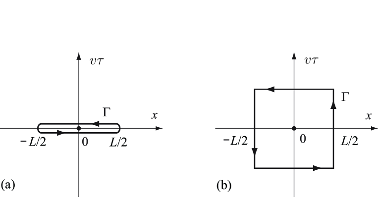
Figure 1: In (a) we show the integration contour $\Gamma$ of Eq. (5.8). It consists of two horizontal segments of length $L$, infinitesimally close to the $x$-axis. The integration contour $\Gamma$ of Eq. (5.14) is shown in (b). It has the shape of a square with side-length $L.$ Both contours are oriented counterclockwise.

We now prove that the expression on the right hand side of Eq. (5.8) is contour-independent. Consider an arbitrary contour enclosing the point $(0,0)$ in the $(x,v\tau)$ plane. To make contact with Eqs. (5.5)–(5.7), we write

$$P=-Tj_{\tau}^{(0)}(x,\tau)\psi(0,0),\qquad Q=Tj_{x}^{(0)}(x,\tau)\psi(0,0),$$ (5.9)

resulting in

$$\frac{\partial Q}{\partial x}-\frac{\partial P}{\partial\tau}=\partial^{\mu}Tj_{\mu}^{(0)}(x,\tau)\psi(0,0).$$ (5.10)

Recall that $j_{x}^{(0)}$ is given by Eqs. (3.15) and (3.50). The $T$-operator in the expression (5.10) commutes with $\partial^{\mu}$ at all points in the $(x,v\tau)$ plane except at the origin of the coordinate system. Therefore

$$\frac{\partial Q}{\partial x}-\frac{\partial P}{\partial\tau}=T\partial^{\mu}j_{\mu}^{(0)}(x,\tau)\psi(0,0)=0,\qquad(x,v\tau)\neq(0,0),$$ (5.11)

where the last equality is ensured by the continuity equation (3.51). We have thus shown that the expression

$$\int_{\Gamma}Pdx+Qd\tau\equiv\int_{\Gamma}-Tj_{\tau}^{(0)}(x,\tau)\psi(0,0)dx+Tj_{x}^{(0)}(x,\tau)\psi(0,0)d\tau\\ =\int_{\Gamma}dx_{\mu}\epsilon^{\mu\nu}Tj_{\nu}^{(0)}(x,\tau)\psi(0,0),$$ (5.12)

where

$$\epsilon_{xx}=\epsilon_{\tau\tau}=0,\qquad\epsilon_{\tau x}=-1,\qquad\epsilon_{x\tau}=1,$$ (5.13)

is contour-independent, unless the contour crosses the origin of the coordinate system. For the contour $\Gamma$ plotted in Fig. 1(a), the equation (5.12) reduces to Eq. (5.8). We have thus proved that the right hand side of Eq. (5.8) is contour-independent, and Eq. (5.4) can be written as follows:

$$\int_{\Gamma}dx_{\mu}\epsilon^{\mu\nu}Tj_{\nu}^{(0)}(x,\tau)\psi(0,0)=-\psi(0,0).$$ (5.14)

Now we choose the shape of the contour $\Gamma$ in Eq. (5.14) as shown in Fig. 1(b): a square with side-length $L$. For large system size, $L,$ the operators $j_{\nu}^{(0)}(x,\tau)$ and $\psi(0,0)$ are well-separated, and their product can be bosonized using Eqs. (4.35), (4.36) and (5.3). Equation (5.14) then reduces to a condition

$$\alpha_{0}=1,$$ (5.15)

as already announced in Eq. (4.38).

The other statement announced in Eq. (4.38), $\beta_{0}=0,$ can be proven by considering the commutation relation of $\psi(x)$ with the momentum operator $P,$ Eq. (1.5):

$$[P,\psi(x)]=i\partial_{x}\psi(x).$$ (5.16)

We write, using Eqs. (3.15) and (3.50),

$$[P,\psi(0)]=\frac{i}{2}\int_{-L/2}^{L/2}\left[j_{x}^{(0)}(x),\psi(0)\right]=-\frac{i}{2}\int_{\Gamma}dx\,Tj_{x}^{(0)}(x,\tau)\psi(0,0),$$ (5.17)

where the contour $\Gamma$ is chosen as shown in Fig. 1(a). Like Eq. (5.8), this expression can be written in a contour-independent form, after which the contour can be deformed to the shape shown in Fig. 1(b), and the operators $j^{(0)}$ and $\psi$ can be bosonized. One gets for $[P,\psi(0)]$ in the bosonized limit

$$[P,\psi(0)]\to\frac{i}{2}\beta_{0}c\mathcal{W}_{1}(0)+\text{h.o.t}$$ (5.18)

On the other hand, it follows from Eq. (5.3) that the operator $\partial_{x}\psi(x)$ in the bosonized limit is proportional to the operator $\partial_{x}\theta\mathcal{W}_{1}(x),$ whose anomalous dimension is higher than that of $\mathcal{W}_{1}(x).$ Thus the only way to satisfy Eq. (5.16) is to require

$$\beta_{0}=0.$$ (5.19)

This completes the proof of Eq. (4.38). It is important to stress that the result (4.38) is valid for any interacting system, the only condition that should be fulfilled is the existence of well-defined number and momentum operators for the system.

5.2 Contour-independent integral identities and the bosonized limit of the Noether currents

We have considered in section 5.1 a contour-invariant integral representation of the operators $[N,\psi(x)]$ and $[P,\psi(x)].$ This method establishes a connection between the short- and long-distance properties of the microscopic theory. The long-distance sector of the theory can be bosonized, with the result of getting explicit answers for the correlation functions. We will continue to work in the present section with the contour-invariant integral representation, studying the Noether currents in the Lieb-Liniger model. Recall that we do not distinguish the Lieb-Liniger and $q$-boson lattice model unless the lattice regularization is required explicitly. Therefore, to shorten notation, we will use in the most cases the continuum space variable $x$ instead of the discrete variable $n.$ The modifications necessary to take into account the discreetness of the space variable are obvious.

We introduce an operator

$$W^{(m)}(x,\tau)=\int_{-L/2}^{x}dx^{\prime}\,j^{(m)}_{\tau}(x^{\prime},\tau),$$ (5.20)

where $j^{(m)}_{\tau}$ is the $\tau$-component of the conserved current $j^{(m)},$ Eq. (3.50). The object which will play a crucial role in our further calculations is

$$G_{\Gamma}^{(n,m)}\equiv\int_{\Gamma}dx\,\left\langle Tj_{\tau}^{(n)}(x,\tau)W^{(m)}(0,0)\right\rangle-d\tau\,\left\langle Tj_{x}^{(n)}(x,\tau)W^{(m)}(0,0)\right\rangle\\ =\int_{\Gamma}dx_{\mu}\epsilon^{\mu\nu}\,\left\langle Tj_{\nu}^{(n)}(x,\tau)W^{(m)}(0,0)\right\rangle,$$ (5.21)

where $\epsilon_{\mu\nu}$ is defined by Eq. (5.13), and $T$ by Eq. (4.11). Like in section 5.1, denote the terms in the integrand of Eq. (5.21) as follows:

$$P=-\left\langle Tj_{\tau}^{(n)}(x,\tau)W^{(m)}(0,0)\right\rangle,\qquad Q=\left\langle Tj_{x}^{(n)}(x,\tau)W^{(m)}(0,0)\right\rangle,$$ (5.22)

therefore,

$$\frac{\partial Q}{\partial x}-\frac{\partial P}{\partial\tau}=\left\langle\partial^{\mu}Tj_{\mu}^{(n)}(x,\tau)W^{(m)}(0,0)\right\rangle.$$ (5.23)

The $T$-operator in this expression commutes with $\partial_{t}$ at all the points of $(x,v\tau)$ plane except the segment

$$\Upsilon=(-L/2\leq x\leq 0,0),$$ (5.24)

therefore

$$\frac{\partial Q}{\partial x}-\frac{\partial P}{\partial\tau}=\left\langle T\partial^{\mu}j_{\mu}^{(n)}(x,\tau)W^{(m)}(0,0)\right\rangle=0,\qquad(x,\tau)\notin\Upsilon,$$ (5.25)

where the last equality is ensured by the continuity equation (3.51).

Let the contour $\Gamma$ in Eq. (5.21) be a square centered around the origin and with the side of length $l$, as shown in Fig. 2a.

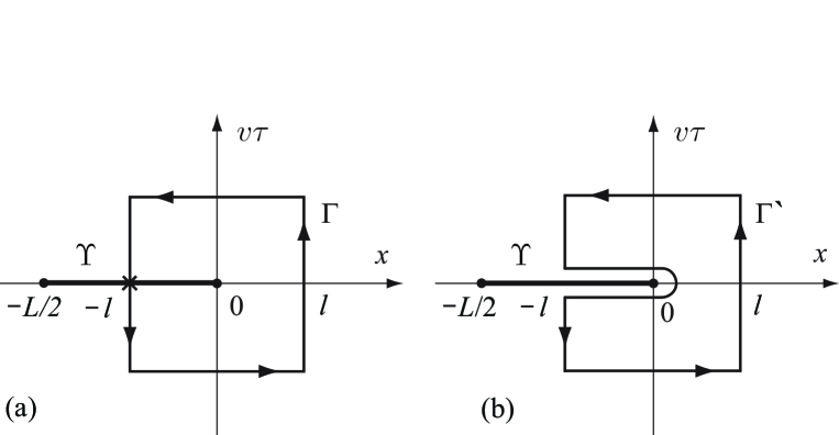
Figure 2: In (a) we show the integration contour $\Gamma$ used in section 5.2. It has the shape of a square with side-length $L.$ The integration contour $\Gamma^{\prime}$ used in section 5.3 is exhibited in (b).

The segment $\Upsilon$ of the $(x,\tau)$ plane is shown there by a thick solid line. The cross in Fig. 2a indicates the intersection point of $\Gamma$ and $\Upsilon.$ Any deformation of $\Gamma$ not changing the position of the intersection point, leaves the value of $G_{\Gamma}^{(n,m)}$ unchanged.

We want to replace the exact currents $j_{\mu}^{(m)}$ entering Eq. (5.21) by their approximate expressions (4.35) and (4.36) obtained within the free boson theory. There is, however, a problem: the operator $j_{\nu}^{(n)}(x,\tau)$ and the operator $j_{\tau}^{(m)}(x^{\prime},0)$ entering $W^{(m)}(0,0)$ are not separated by the asymptotically large space-time interval in a vicinity of the intersection point of $\Gamma$ and $\Upsilon$, and one cannot apply Eqs. (4.35) and (4.36) to the operator $j_{\nu}^{(n)}(x,\tau)j_{\tau}^{(m)}(x^{\prime},0).$ To circumvent this problem we use the following trick: Introduce an operator

$$\tilde{W}^{(m)}(x,\tau)\equiv-\int_{x}^{L/2}dx^{\prime}\,j_{\tau}^{(m)}(x^{\prime},\tau).$$ (5.26)

Combining Eqs. (5.20) and (5.26), one gets

$$W^{(m)}(x,\tau)-\tilde{W}^{(m)}(x,\tau)=\int_{-L/2}^{L/2}dx^{\prime}\,j_{\tau}^{(m)}(x^{\prime},\tau)=I_{m}-\langle I_{m}\rangle,$$ (5.27)

where $I_{m}$ are the integrals of motion of the $q$-boson lattice model, discussed in section 2.3. Then, we split the contour $\Gamma$ into two parts:

$$\Gamma=\left\{\begin{array}[]{cc}\Gamma_{+}&x>0\\ \Gamma_{-}&x<0\end{array}\right..$$ (5.28)

Using Eqs. (5.26)–(5.28) we rewrite the expression (5.21) in the following form

$$G_{\Gamma}^{(n,m)}=\int_{\Gamma_{+}}dx_{\mu}\epsilon^{\mu\nu}\left\langle Tj_{\nu}^{(n)}(x,\tau)W^{(m)}(0,0)\right\rangle\\ +\int_{\Gamma_{-}}dx_{\mu}\epsilon^{\mu\nu}\left\langle Tj_{\nu}^{(n)}(x,\tau)\tilde{W}^{(m)}(0,0)\right\rangle+\int_{\Gamma_{-}}dx_{\mu}\epsilon^{\mu\nu}\left\langle Tj_{\nu}^{(n)}(x,\tau)(I_{m}-\langle I_{m}\rangle)\right\rangle.$$ (5.29)

The third term on the right hand side of Eq. (5.29) vanishes because the ground state $|\mathrm{gs}\rangle$ is an eigenfunction of $I_{m}.$ In the first (second) term the distance between the local field $j_{\nu}^{(n)}(x,\tau)$ and the local field $j_{\tau}^{(m)}(x^{\prime},0)$ entering the operator $W^{(m)}(0,0)$ (the operator $\tilde{W}^{(m)}(0,0)$) is larger than $l.$

A nontrivial output from Eq. (5.29) comes in the limit

$$L\to\infty,\qquad l\to\infty,\qquad\frac{l}{L}\to 0.$$ (5.30)

Since the operators $j_{\nu}^{(n)}(x,\tau)$ and $j_{\tau}^{(m)}(x^{\prime},0)$ entering Eq. (5.29) are separated by a distance larger than $l,$ one can use the bosonized expressions (4.35) and (4.36) in the limit (5.30). Taking into account Eq. (4.24), one gets after some algebra

$$G_{\Gamma}^{(n,m)}=-\frac{Kv}{\pi}(\alpha_{n}\beta_{m}+\alpha_{m}\beta_{n}).$$ (5.31)

5.3 Contour-independent integral identities: the main result

In present section we relate the ground-state average of some nontrivial local operator of the $q$-boson lattice model to the properties of this model in the bosonized limit. Establishing this relation, Eq. (5.40), we get all necessary information for the calculation of the function $g_{3}(\gamma),$ Eq. (1.9).

We use the techniques developed in sections 5.1 and 5.2. Choose the contour $\Gamma^{\prime}$ in $(x,v\tau)$ plane as shown in Fig. 2(b). Namely, $\Gamma^{\prime}$ consists of the two horizontal segments, $(-l\leq x\leq\epsilon,+0)$ and $(-l\leq x\leq\epsilon,-0)$, and the square with the side $l,$ centered around the origin. The latter part is just the contour $\Gamma$ used in sections 5.1 and 5.2. Using the techniques developed there we write

$$G_{\Gamma}^{(n,m)}+\int_{-l}^{\epsilon}dx\left\langle\left[j^{(n)}_{\tau}(x,0),W^{(m)}(0,0)\right]\right\rangle=0.$$ (5.32)

The parameter $\epsilon>0$ plays the role of a regularization parameter, as it is necessary to treat unambiguously the behavior of the integral in the vicinity of $x=0.$ We shall work with Eq. (5.32) in the limit (5.30), and we can therefore use Eq. (5.31) to get

$$\int_{-l}^{\epsilon}dx\int_{-L/2}^{0}dx^{\prime}\,\left\langle\left[j_{\tau}^{(n)}(x),j_{\tau}^{(m)}(x^{\prime})\right]\right\rangle=\frac{Kv}{\pi}(\alpha_{m}\beta_{n}+\alpha_{n}\beta_{m}).$$ (5.33)

We remind the reader that we write the lattice regularization explicitly only when it is necessary. Here is the proper place to do it. Equation (5.33) then takes the form

$$\delta^{2}\sum_{k=-l\delta^{-1}}^{\epsilon\delta^{-1}}\sum_{p=-L\delta^{-1}/2}^{0}\left\langle\left[j_{\tau}^{(n)}(k),j_{\tau}^{(m)}(p)\right]\right\rangle=\frac{Kv}{\pi}(\alpha_{m}\beta_{n}+\alpha_{n}\beta_{m}).$$ (5.34)

Let us take the limit (5.30), keeping $\delta^{-1}$ finite. Therefore

$$L\delta^{-1}\to\infty,\qquad l\delta^{-1}\to\infty$$ (5.35)

in Eq. (5.34). We then choose the parameter $\epsilon$ such that

$$\epsilon\delta^{-1}>m.$$ (5.36)

We set $n=-1$ and $m=2$ in Eq. (5.34). The local operators $j_{\tau}^{(-1)}(k)$ and $j_{\tau}^{(2)}(p)$ are defined by Eqs. (2.45), (2.46), (2.51), and (3.50). Using these definitions, we calculate the expression on the left hand side of Eq. (5.34) under the conditions (5.35) and (5.36):

$$\frac{\delta^{2}}{\chi^{2}}\left(1-\frac{\chi^{2}}{2}\right)^{-1}\sum_{k=-l\delta^{-1}}^{\epsilon\delta^{-1}}\sum_{p=-L\delta^{-1}/2}^{0}\left\langle\left[j_{\tau}^{(-1)}(k),j_{\tau}^{(2)}(p)\right]\right\rangle\\ =\left\langle-\chi^{2}B^{\dagger}_{j}B_{j+1}+\chi^{4}B^{\dagger}_{j}B^{\dagger}_{j}B_{j}B_{j+1}\right\rangle.$$ (5.37)

Comparing this result with the right hand side of Eq. (5.34) one gets

$$\langle-\chi^{2}B^{\dagger}_{j}B_{j+1}+\chi^{4}B^{\dagger}_{j}B^{\dagger}_{j}B_{j}B_{j+1}\rangle=\frac{1}{\chi^{2}}\left(1-\frac{\chi^{2}}{2}\right)^{-1}\frac{Kv}{\pi}(\alpha_{-1}\beta_{2}+\alpha_{2}\beta_{-1}).$$ (5.38)

This expression relates the ground-state average of the local operator of the microscopic model to the properties of this model in the bosonized limit.

Let us combine Eqs. (5.38), (2.45), and (2.77)

$$\langle B^{\dagger}_{j}B^{\dagger}_{j}B_{j}B_{j+1}\rangle=\frac{\delta}{\chi^{4}}\frac{\langle I_{1}\rangle}{L}+\frac{1}{\chi^{6}}\left(1-\frac{\chi^{2}}{2}\right)^{-1}\frac{Kv}{\pi}(\alpha_{-1}\beta_{2}+\alpha_{2}\beta_{-1}),$$ (5.39)

and substitute into Eq. (5.39) the results (4.48), (4.49) and (4.53). This gives

$$\langle B^{\dagger}_{j}B^{\dagger}_{j}B_{j}B_{j+1}\rangle=\frac{\delta}{\chi^{4}}\frac{\langle I_{1}\rangle}{L}\left[1+\left(1-\frac{\chi^{2}}{2}\right)^{-1}\frac{1}{\chi^{2}}\left(\frac{\partial\langle I_{2}\rangle}{\partial\langle I_{0}\rangle}-2\frac{\langle I_{2}\rangle}{\langle I_{1}\rangle}\frac{\partial\langle I_{1}\rangle}{\partial\langle I_{0}\rangle}\right)\right].$$ (5.40)

6 Three-body local correlation function

Working with the $q$-boson lattice model, we obtained in previous sections all the formulas necessary to calculate $g_{3}(\gamma).$ The remaining task is to take the continuum limit in these formulas and to collect all them together. The limit is taken in section 6.1 and the formulas are collected together in section 6.2.

6.1 Properties of $\langle I_{m}\rangle$ close to the continuum limit

In this section we continue our studies of $\langle I_{m}\rangle$ in the $q$-boson lattice model, started in section 2.4. The continuum limit (2.19) of the $q$-boson lattice model gives the Lieb-Liniger model, Eq. (1.1). The limit in which we are interested is the continuum limit together with the extra condition $L\to\infty,$ coming from Eq. (5.30). Therefore, we consider

$$\delta\to 0,\qquad M\to\infty,\qquad\kappa\to 0,\qquad L\to\infty,$$ (6.1)

where

$$L=\delta M,\qquad q=e^{\kappa},\qquad c/2=\kappa\delta^{-1}.$$ (6.2)

Let us renormalize the quasi-momenta $p_{j}$ used in section 2.4:

$$k_{j}=\delta^{-1}p_{j}.$$ (6.3)

The kernel (2.86) can be represented in the limit (6.1) as follows

$$K(p)=\delta^{-1}K(k),\qquad K(k)=\frac{2c}{c^{2}+k^{2}}+\frac{\delta^{2}}{6}c+\frac{\delta^{4}}{360}\left(3ck^{2}-c^{3}\right)+\dots.$$ (6.4)

When written in terms of the variables $k_{j},$ the normalization condition (2.84) becomes

$$n=\int_{-\Lambda(\delta)}^{\Lambda(\delta)}dk\,\rho(k,\delta),$$ (6.5)

and the Lieb-Liniger equation (2.85) becomes

$$\rho(k,\delta)-\frac{1}{2\pi}\int_{-\Lambda(\delta)}^{\Lambda(\delta)}d\tilde{k}\,K(k-\tilde{k})\rho(\tilde{k},\delta)=\frac{1}{2\pi}.$$ (6.6)

Here the ground-state density $D$ is defined by Eq. (2.79). Note that the functions $\Lambda$ and $\rho$ in Eqs. (6.5) and (6.6) are different from those used in Eqs. (2.84) and (2.86). We, however, use the same symbols for these two couples, since we shall work with Eqs. (6.5) and (6.6) exclusively.

The ground state expectation values of $I_{1}$ and $I_{2},$ Eqs. (2.87) and (2.88), can be represented in the limit (6.1) as follows

$$\frac{\langle I_{1}\rangle}{L}=\chi^{2}\left(D-\frac{\delta^{2}}{2!}h_{2}+\frac{\delta^{4}}{4!}h_{4}+\dots\right),$$ (6.7)

and

$$\frac{\langle I_{2}\rangle}{L}=\chi^{2}\left(1-\frac{\chi^{2}}{2}\right)\left(D-\frac{(2\delta)^{2}}{2!}h_{2}+\frac{(2\delta)^{4}}{4!}h_{4}+\dots\right),$$ (6.8)

where

$$h_{m}(\delta)=\int_{-\Lambda(\delta)}^{\Lambda(\delta)}dk\,\rho(k,\delta)k^{m}.$$ (6.9)

Equations (6.7) and (6.8) are not series expansions in powers of $\delta$ since the functions $h_{m}$ themselves depend on $\delta$ through the quasi-momentum distribution $\rho$ and through $\Lambda.$ The series expansion of $h_{m}$ in powers of $\delta$ is

$$h_{m}(\delta)=h_{m}^{(0)}+\delta^{2}h_{m}^{(1)}+\dots$$ (6.10)

Let us consider Eqs. (6.5) and (6.6) at $\delta=0:$

$$D=\int_{-\Lambda(0)}^{\Lambda(0)}dk\,\rho(k,0)$$ (6.11)

and

$$\rho(k,0)-\frac{1}{2\pi}\int_{-\Lambda(0)}^{\Lambda(0)}d\tilde{k}\,\frac{2c}{c^{2}+(k-\tilde{k})^{2}}\rho(\tilde{k},0)=\frac{1}{2\pi}.$$ (6.12)

Following Ref. [5] we change the variables

$$k=\Lambda(0)z,\qquad c=\Lambda(0)\alpha,\qquad\rho(\Lambda(0)z,0)=\sigma(z).$$ (6.13)

When written in these variables, Eqs. (6.11) and (6.12) become Eqs. (1.15) and (1.14), respectively. The function $h_{m}^{(0)}$ introduced by (6.10) can be written as

$$h_{m}^{(0)}(D,c)=D^{m+1}\epsilon_{m}\left(\gamma\right),$$ (6.14)

where the function $\epsilon_{m}(\gamma),$ given by Eq. (1.13), depends on the dimensionless parameter $\gamma,$ Eq. (1.7), only. One verifies readily that $h_{m}^{(0)}$ satisfies the following differential equation

$$D\frac{\partial}{\partial D}h_{m}^{(0)}+c\frac{\partial}{\partial c}h_{m}^{(0)}-(m+1)h_{m}^{(0)}=0.$$ (6.15)

Next, we consider the solution of Eqs. (6.5) and (6.6) to second order in $\delta.$ Substituting Eq. (6.4) into (6.6) and keeping the terms up to the order of $\delta^{2}$ we find

$$\rho(k,\delta)-\frac{1}{2\pi}\int_{-\Lambda(\delta)}^{\Lambda(\delta)}d\tilde{k}\frac{2c}{c^{2}+(k-\tilde{k})^{2}}\rho(\tilde{k},\delta)=\frac{1}{2\pi}\left(1+\frac{c\delta^{2}}{6}D\right).$$ (6.16)

By rescaling the quasi-momentum distribution function

$$\rho(k,\delta)=\left(1+\frac{c\delta^{2}}{6}D\right)\tilde{\rho}(k,\delta)$$ (6.17)

we find that $\tilde{\rho}(k,\delta)$ satisfies the integral equation

$$\tilde{\rho}(k,\delta)-\frac{1}{2\pi}\int_{-\Lambda(\delta)}^{\Lambda(\delta)}d\tilde{k}\frac{2c}{c^{2}+(k-\tilde{k})^{2}}\tilde{\rho}(\tilde{k},\delta)=\frac{1}{2\pi}$$ (6.18)

with the condition (6.5) renormalized as follows:

$$D\left(1-\frac{c\delta^{2}}{6}D\right)=\int_{-\Lambda(\delta)}^{\Lambda(\delta)}dk\,\tilde{\rho}(k,\delta).$$ (6.19)

It is clear from comparison of Eqs. (6.19) and (6.18) with Eqs. (6.11) and (6.12) that the function $h_{2},$ Eq. (6.9), can be represented to order $\delta^{2}$ as follows

$$h_{2}(D,c)=\left(1+\frac{c\delta^{2}D}{6}\right)\int_{-\Lambda(\delta)}^{\Lambda(\delta)}dk\,k^{2}\tilde{\rho}(k,\delta)=\left(1+\frac{c\delta^{2}D}{6}\right)h_{2}^{(0)}\left(D-\frac{c\delta^{2}D^{2}}{6},c\right).$$ (6.20)

Expanding this equation and dropping terms of higher order than $\delta^{2},$ we get

$$h_{2}=h_{2}^{(0)}+\frac{c\delta^{2}D}{6}\left(h_{2}^{(0)}-D\frac{\partial h_{2}^{(0)}}{\partial D}\right).$$ (6.21)

Finally, combining Eqs. (6.15) and (6.21), we get the following differential equation for $h_{2}:$

$$D\frac{\partial h_{2}}{\partial D}+c\frac{\partial h_{2}}{\partial c}-3h_{2}=\frac{c\delta^{2}D}{3}\left(h_{2}-D\frac{\partial h_{2}}{\partial D}\right)+\dots$$ (6.22)

where we have dropped all the terms of the order higher than $\delta^{2}.$

6.2 Three-body local correlation function: the result

We are now in the position to derive the main result of this paper: equation (1.12) for the three-body local correlation function $g_{3}(\gamma),$ Eq. (1.9), of the Lieb-Liniger model in the limit (1.11). To do this, we take the limit (6.1) in the ground-state averages of local operators of the $q$-boson model, which were obtained in earlier sections. The corresponding calculations are straightforward but rather lengthy, and we shall only sketch their main steps.

The desired ground state expectation value (1.9) in the Lieb-Liniger model can be obtained by taking the limit (6.1) of the following $q$-boson local field:

$$\left\langle(1-\chi^{2})B^{\dagger}_{j}B^{\dagger}_{j}B_{j}B_{j+1}+\left(1-\frac{\chi^{2}}{2}\right)q\frac{d}{dq}(B_{j}^{\dagger}B_{j+1})\right\rangle\\ =-\frac{c\delta^{4}}{3}\left[\langle\psi^{\dagger}(x)^{3}\psi(x)^{3}\rangle+\dots\right],$$ (6.23)

where the dots denote terms of higher order in $\delta.$ To prove Eq. (6.23) we use Eq. (2.96) and then take the limit (6.1) in the way discussed in section 2.2, Eqs. (2.22)–(2.25). After rather lengthy algebra we got the right hand side of Eq. (6.23).

As our next step we rewrite the left hand side of Eq. (6.23) using the identities (5.40) and (2.92)

$$\left\langle(1-\chi^{2})B^{\dagger}_{j}B^{\dagger}_{j}B_{j}B_{j+1}+\left(1-\frac{\chi^{2}}{2}\right)q\frac{d}{dq}(B_{j}^{\dagger}B_{j+1})\right\rangle=\left(1-\frac{\chi^{2}}{2}\right)q\frac{d}{dq}\left(\frac{\langle I_{1}\rangle}{L}\frac{\delta}{\chi^{2}}\right)\\ +(1-\chi^{2})\frac{\delta}{\chi^{4}}\frac{\langle I_{1}\rangle}{L}\left[1+\left(1-\frac{\chi^{2}}{2}\right)^{-1}\frac{1}{\chi^{2}}\left(\frac{\partial\langle I_{2}\rangle}{\partial\langle I_{0}\rangle}-2\frac{\langle I_{2}\rangle}{\langle I_{1}\rangle}\frac{\partial\langle I_{1}\rangle}{\partial\langle I_{0}\rangle}\right)\right]$$ (6.24)

and take the limit (6.1) in the resulting expression. Substituting the expansions (6.7) and (6.8) into the right hand side of Eq. (6.24) one arrives at

$$\left\langle(1-\chi^{2})B^{\dagger}_{j}B^{\dagger}_{j}B_{j}B_{j+1}+\left(1-\frac{\chi^{2}}{2}\right)q\frac{d}{dq}(B_{j}^{\dagger}B_{j+1})\right\rangle\\ =\left(\frac{\delta^{3}}{2}-\frac{\delta^{2}}{c}\right)\left(D\frac{\partial h_{2}}{\partial D}+c\frac{\partial h_{2}}{\partial c}-3h_{2}\right)-\delta^{4}\left[\frac{c}{12}\left(D\frac{\partial h_{2}}{\partial D}+3c\frac{\partial h_{2}}{\partial c}-3h_{2}\right)\right.\\ -\left.\frac{1}{12c}\left(7D\frac{\partial h_{4}}{\partial D}+c\frac{\partial h_{4}}{\partial c}-15h_{4}\right)+\frac{h_{2}}{c}\frac{\partial h_{2}}{\partial D}\right].$$ (6.25)

where we have dropped terms of higher order than $\delta^{4}.$ Using Eq. (6.22) to transform the first term on the right hand side of Eq. (6.25) one can see that the expansion (6.25) starts from the terms of order $\delta^{4}.$ Comparing these leading order terms with the term written explicitly on the right hand side of Eq. (6.23) and replacing $h_{m}$ with $h_{m}^{(0)},$ Eq. (6.14), one gets after some algebra the final result, Eq. (1.12).

Acknowledgments

The authors would like to thank N.M. Bogoliubov and V. Tarasov for helpful discussions. M.B. Zvonarev’s work was supported by the Danish Technical Research Council via the Framework Programme on Superconductivity and by the Swiss National Fund for research under MANEP and Division II.

References

- [1] Tolra B L, O’Hara K M, Huckans J H, Phillips W D, Rolston S L and Porto J V 2004 Observation of Reduced Three-Body Recombination in a Correlated 1D Degenerate Bose Gas Phys Rev Lett 92 190401
- [2] Cheianov V V, Smith H and Zvonarev M B 2005 Exact results for three-body correlations in a degenerate one-dimensional Bose gas e-print cond-mat/0506609
- [3] Smirnov F A 1992 Form Factors in Completely Integrable Models of Quantum Field Theory (World Scientific: Singapore)
- [4] Lukyanov S and Zamolodchikov Alexander 1997 Exact expectation values of local fields in the quantum sine-Gordon model Nucl Phys. B 493 [FS] 571–587
- [5] Lieb E H and Liniger W 1963 Exact Analysis of an Interacting Bose Gas. I. The General Solution and the Ground State Phys Rev 130 1605–1616
- [6] Amico L and Korepin V E 2004 Universality of the one-dimensional Bose gas with delta interaction Annals of Physics 314 496–507
- [7] Bogoliubov N M, Bullough R K and Pang G D 1993 Exact solution of a -boson hopping model Phys Rev B 47 11495–11498.
- [8] Bogoliubov N M, Izergin A G and Kitanine N A 1998 Correlation functions for a strongly correlated boson system Nucl Phys B 516 [FS] 501–528
- [9] Korepin V E, Bogoliubov N M and Izergin A G 1993 Quantum Inverse Scattering Method and Correlation Functions (Cambridge: Cambridge University Press)
- [10] Weinberg S 1995 The quantum theory of fields (Cambridge: Cambridge University Press)
- [11] Olshanii M and Dunjko V 2003 Short-Distance Correlation Properties of the Lieb-Liniger System and Momentum Distributions of Trapped One-Dimensional Atomic Gases Phys. Rev. Lett. 91 090401
- [12] Giamarchi T 2004 Quantum Physics in One Dimension (Oxford University Press)
- [13] Gogolin A O, Nersesyan A A and Tsvelik A M 1993 Bosonization and Strongly Correlated Systems (Cambridge: Cambridge University Press)
- [14] Haldane F D M 1981 Demonstration of the “Luttinger Liquid” character of Bethe-ansatz soluble models of 1-D quantum fluids Phys Lett A 81 153–155