Detecting the quantum zero-point motion of vortices in the cuprate superconductors

Abstract

We explore the experimental implications of a recent theory of the quantum dynamics of vortices in two-dimensional superfluids proximate to Mott insulators. The theory predicts modulations in the local density of states in the regions over which the vortices execute their quantum zero point motion. We use the spatial extent of such modulations in scanning tunnelling microscopy measurements (Hoffman et al, Science 295, 466 (2002)) on the vortex lattice of Bi₂Sr₂CaCu₂O_8+δ to estimate the inertial mass of a point vortex. We discuss other, more direct, experimental signatures of the vortex dynamics.

, , and

1 Introduction

It is now widely accepted that superconductivity in the cuprates is described, as in the standard Bardeen-Cooper-Schrieffer (BCS) theory, by the condensation of charge $-2e$ Cooper pairs of electrons. However, it has also been apparent that vortices in the superconducting state are not particularly well described by BCS theory. While elementary vortices do carry the BCS flux quantum of $hc/2e$, the local electronic density of states in the vortex core, as measured by scanning tunnelling microscopy (STM) experiments, has not been explained naturally in the BCS framework. Central to our considerations here are the remarkable STM measurements of Hoffman et al. [1] (see also Refs. [2, 3]) who observed modulations in the local density of states (LDOS) with a period of approximately 4 lattice spacings in the vicinity of each vortex core of a vortex lattice in Bi₂Sr₂CaCu₂O_8+δ.

This paper shall present some of the physical implications of a recent theory of two-dimensional superfluids in the vicinity of a quantum phase transition to a Mott insulator [4, 5] (see also Ref. [6]). By ‘Mott insulator’ we mean here an incompressible state which is pinned to the underlying crystal lattice, with an energy gap to charged excitations. In the Mott insulator, the average number of electrons per unit cell of the crystal lattice, $n_{MI}$, must be a rational number. If the Mott insulator is not ‘fractionalized’ and if $n_{MI}$ is not an even integer, then the Mott insulator must also spontaneously break the space group symmetry of the crystal lattice so that the unit cell of the Mott insulator has an even integer number of electrons. There is evidence that the hole-doped cuprates are proximate to a Mott insulator with $n_{MI}=7/8$ [7], and such an assumption will form the basis of our analysis of the STM experiments on Bi₂Sr₂CaCu₂O_8+δ. The electron number density in the superfluid state, $n_{S}$, need not equal $n_{MI}$ and will be assumed to take arbitrary real values, but not too far from $n_{MI}$.

A key ingredient in our analysis will be the result that the superfluid carries a subtle quantum order, which is distinct from Landau-Ginzburg order of a Cooper pair condensate. In two dimensions, vortices are point-like excitations, and are therefore bona fide quasiparticle excitations of the superfluid. The quantum order is reflected in the wavefunction needed to describe the motion of the vortex quasiparticle. For $n_{MI}$ not an even integer, the low energy vortices appear in multiple degenerate flavors, and the space group symmetry of the underlying lattice is realized in a projective unitary representation that acts on this flavor space. Whenever a vortex is pinned (either individually due to impurities, or collectively in a vortex lattice), the space group symmetry is locally broken, and hence the vortex necessarily chooses a preferred orientation in its flavor space. As shown in Ref. [4], this implies the presence of modulations in the LDOS in the spatial region over which the vortex executes its quantum zero point motion [8]. The short-distance structure and period of the modulations is determined by that of the Mott insulator at density $n_{MI}$, while its long-distance envelope is a measure of the amplitude of the vortex wavefunction (see Fig. 1).

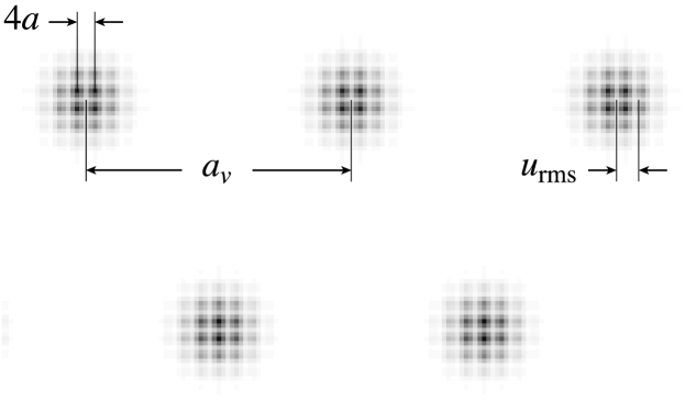
Figure 1: Schematic of the modulations in the LDOS of a vortex lattice. The short distance modulations in each vortex halo are determined by the orientation of the vortex in flavor space, as discussed in Ref. [4]. The envelope of these modulations is $|\Psi({\bf r}_{j})|^{2}$ where $\Psi$ is the wavefunction of the vortices, and its characteristics are computed in the present paper.

Consequently, the size of the region where the modulations are present is determined by the inertial mass of the vortex. Here we will show how these ideas can be made quantitatively precise, and use current experiments to obtain an estimate of the vortex mass, $m_{v}$. There have been a number of theoretical discussions of $m_{v}$ using BCS theory [9, 10, 11, 12, 13, 14, 15], and they lead to the order of magnitude estimate $m_{v}\sim m_{e}(k_{F}\xi)^{2}$, where $m_{e}$ is the electron mass, $k_{F}$ is the Fermi wavevector, and $\xi$ is the BCS coherence length.

2 Vortex equations of motion

We begin with a very simple, minimal model computation of the vortex dynamics, in which retardation, dissipation, and inter-layer Coulomb interactions will be neglected. This serves the purpose of exposing the basic physics. The following section will present a much more complete derivation, in which these effects will be re-instated, and the connection to the field theory analysis of Refs. [4] will also be made explicit.

Consider a system of point vortices moving in a plane at positions ${\bf r}_{j}$, where $j$ is a label identifying the vortices. We do not explicitly identify the orientation of each vortex in flavor space, because we are interested here only in the long-distance envelope of the LDOS modulations; the flavor orientation does not affect the interactions between well-separated vortices, and so plays no role in determining the wavefunction of the vortex lattice. In a Galilean-invariant superfluid, the vortices move under the influence of the Magnus force

$$m_{v}\frac{d^{2}{\bf r}_{j}}{dt^{2}}=\frac{hn_{S}}{2a^{2}}\left({\bf v}_{s}({\bf r}_{j})-\frac{d{\bf r}_{j}}{dt}\right)\times\hat{\bf z},$$ (1)

where $t$ is time, $h=2\pi\hbar$ is Planck’s constant, ${\bf v}_{s}({\bf r})$ is the superfluid velocity at the position ${\bf r}$, and $n_{S}/a^{2}$ is the electron number density per unit area ($a^{2}$ is the area of a unit cell of the underlying lattice). One point of view is that the force in Eq. (1) is that obtained from classical fluid mechanics after imposing the quantization of circulation of a vortex. However, Refs. [16] emphasized the robust topological nature of the Magnus force and its connection to Berry phases, and noted that it applied not only to superfluids of bosons, but quite generally to superconductors of paired electrons. Here, we need the modification of Eq. (1) by the periodic crystal potential and the proximate Mott insulator. This was implicit in the results of Ref. [4], and we present it in more physical terms. It is useful to first rewrite Eq. (1) as

$$m_{v}\frac{d^{2}{\bf r}_{j}}{dt^{2}}={\bf F}_{E}(j)+{\bf F}_{B}(j),$$ (2)

where ${\bf F}_{E}$ is the first term proportional to ${\bf v}_{s}$ and ${\bf F}_{B}$ is the second term. Our notation here is suggestive of a dual formulation of the theory in which the vortices appear as ‘charges’, and these forces are identified as the ‘electrical’ and ‘magnetic’ components. In the Galilean invariant superfluid, the values of ${\bf F}_{E}$ and ${\bf F}_{B}$ are tied to each other by a Galilean transformation. However, with a periodic crystal potential, this constraint no longer applies, and their values renormalize differently as we now discuss.

The influence of the crystal potential on ${\bf F}_{E}$ is simple, and replaces the number density of electrons, $n_{S}$, by the superfluid density. Determining ${\bf v}_{s}({\bf r}_{j})$ as a sum of contributions from the other vortices, we obtain [17]

$${\bf F}_{E}(j)=2\pi\rho_{s}\sum_{k(\neq j)}\frac{{\bf r}_{j}-{\bf r}_{k}}{|{\bf r}_{j}-{\bf r}_{k}|^{2}}\;,$$ (3)

where $\rho_{s}$ is the superfluid stiffness (in units of energy). It is related to the London penetration depth, $\lambda$, by

$$\rho_{s}=\frac{\hbar^{2}c^{2}d}{16\pi e^{2}\lambda^{2}},$$ (4)

where $d$ is the interlayer spacing.

The modification of ${\bf F}_{B}$ is more subtle. This term states that the vortices are ‘charges’ moving in a ‘magnetic’ field with $n_{S}/2$ ‘flux’ quanta per unit cell of the periodic crystal potential. In other words, the vortex wavefunction is obtained by diagonalizing the Hofstadter Hamiltonian which describes motion of a charged particle in the presence of a magnetic field and a periodic potential. As argued in Ref. [4], it is useful to examine this motion in terms of the deviation from the rational ‘flux’ $n_{MI}/2=p/q$ ($p$, $q$ are relatively prime integers) associated with the proximate Mott insulator. The low energy states of the rational flux Hofstadter Hamiltonian have a $q$-fold degeneracy, and this constitutes the vortex flavor space noted earlier [18]. However, these vortex states describe particle motion in zero ‘magnetic’ field, and only the deficit $(n_{S}-n_{MI})/2$ acts as a ‘magnetic flux’. This result is contained in the action in Eq. (2.46) of Ref. [4] (see also Eq. (17) below), which shows that the dual gauge flux fluctuates about an average flux determined by $(n_{S}-n_{MI})$. The action in Ref. [4] has a ‘relativistic’ form appropriate to a system with equal numbers of vortices and anti-vortices. Here, we are interested in a system of vortices induced by an applied magnetic field, and can neglect anti-vortices; so we should work with the corresponding ‘non-relativistic’ version of Eq. (2.46) of Ref. [4]. In its first-quantized version, this ‘non-relativistic’ action for the vortices leads to the ‘Lorentz’ force in Eq. (2) given by

$${\bf F}_{B}(j)=-\frac{h(n_{S}-n_{MI})}{2a^{2}}\frac{d{\bf r}_{j}}{dt}\times\hat{\bf z},$$ (5)

If the density of the superfluid equals the commensurate density of the Mott insulator, then ${\bf F}_{B}=0$; however, ${\bf F}_{E}$ remains non-zero because we can still have $\rho_{s}\neq 0$ in the superfluid. These distinct behaviors of ${\bf F}_{E,B}$ constitute a key difference from Galilean-invariant superfluids. In experimental studies of vortex motion in superconductors [19], a force of the form of Eq. (5) is usually quoted in terms of a ‘Hall drag’ co-efficient per unit length of the vortex line, $\alpha$; Eq. (5) implies

$$\alpha=-\frac{h(n_{S}-n_{MI})}{2a^{2}d}.$$ (6)

Thus the periodic potential has significantly reduced the magnitude of $\alpha$ from the value nominally expected [20] by subtracting out the density of the Mott insulator. A smaller than expected $|\alpha|$ is indeed observed in the cuprates [19]. It is worth emphasizing that ${\bf F}_{B}$ (but not ${\bf F}_{E}$) is an intrinsic property of a single vortex. Moreover, we expect that, taken together, the relation Eq. (6) and the flavor degeneracy $q$ are robust “universal” measures of the quantum order of a clean superconductor, independent of details of the band structure, etc.

3 Derivation from field theory

We will now rederive the results of the previous section from a more sophisticated perspective. We will use a field theoretic approach to derive an effective action for the vortices, a limiting case of which will be equivalent to the equations of motion already presented. The effective action will include retardation effects, and can be easily extended to include inter-layer interactions and dissipation.

Our starting point is a model of ordinary bosons on the square lattice interacting via the long-range Coulomb interaction. Following Ref. [4] we will briefly review a duality mapping of this model into a field theory for vortices in a superfluid of bosons which is in the vicinity of a transition to a Mott insulator. The density of bosons per unit cell of the underlying lattice is $\rho_{B}=n_{B}/a^{2}$, while the density of bosons in the Mott insulator is $\rho_{MI}=n_{MI}^{(B)}/a^{2}=(p/q)/a^{2}$; here $a^{2}$ is the unit cell area of the underlying lattice. Closely related field theories apply to models of electrons on the square lattice appropriate to the cuprate superconductors [5, 21], with the boson density replaced by the corresponding density of Cooper pairs; the needed extensions do not modify any of the results presented below. It should be noted that since two electrons pair to form one Cooper pair the average number of electrons in the Mott insulating state is $n_{MI}=2n_{MI}^{(B)}$ (and the average number of electrons in the superfluid phase is $n_{s}=2n_{B}$).

In zero applied magnetic field, the Hamiltonian of our system is given by

$$\mathcal{H}=-\rho_{s}\sum_{i\alpha}\cos\left(\Delta_{\alpha}\hat{\phi}_{i}\right)+\frac{e^{\ast\,2}}{2}\sum_{i\neq j}\frac{(\hat{n}_{i}-n_{B})(\hat{n}_{j}-n_{B})}{|{\bf r}_{i}-{\bf r}_{j}|}\;,$$ (7)

where $\rho_{s}$ is the superfluid stiffness and $-e^{\ast}$ ($=-2e$) is the charge of a boson (Cooper pair). The bosons are represented by conjugate rotor and number operators $\hat{\phi}_{i}$ and $\hat{n}_{i}$ which live on the sites $i$ of the square lattice (with position vector ${\bf r}_{i}$) and satisfy the commutation relations

$$[\hat{\phi}_{i},\hat{n}_{j}]=i\delta_{ij}\;.$$ (8)

We subtract the average boson density $n_{B}$ from the number operators $\hat{n}_{i}$ to account for global charge neutrality of the system. Finally, we have introduced the discrete lattice derivative $\Delta_{\alpha}\hat{\phi}_{i}=\hat{\phi}_{i+\alpha}-\hat{\phi}_{i}$ along one of the two spatial directions $\alpha=x$ or $y$.

3.1 Dual lattice representation

Let us now briefly review the duality analysis of the above model with special emphasis on the long-range Coulomb interaction. Following Ref. [4] we represent the partition function of $\mathcal{H}$ as a Feynman path integral by inserting complete sets of eigenstates to the number operators $\hat{n}_{i}$ at times separated by the imaginary time slice $\Delta\tau$. While the Coulomb interaction term is diagonal in this basis, the hopping term in $\mathcal{H}$ can be easily evaluated by making use of the Villain representation

$$\exp\left(\rho_{s}\Delta\tau\cos\left(\Delta_{\alpha}\hat{\phi}_{i}\right)\right)\rightarrow\sum_{\{J_{i\alpha}\}}\exp\left(-\frac{J_{i\alpha}^{2}}{2\rho_{s}\Delta\tau}+iJ_{i\alpha}\Delta_{\alpha}\hat{\phi}_{i}\right)\;.$$ (9)

Here, we have set $\hbar=1$ and have dropped an unimportant normalization constant which we will also do in the following. The $J_{i\alpha}$ are integer variables residing on the links of the direct lattice, representing the current of the bosons.

Extending the lattice index $i$ to spacetime and introducing the integer-valued boson current in spacetime, $J_{i\mu}\equiv(n_{i},J_{ix},J_{iy})$, the partition function can be written as

$$\mathcal{Z}={\sum_{\{J_{i\mu}\}}}^{\prime}\exp\left(-\frac{1}{2\Delta\tau\rho_{s}}\sum_{i\alpha}J_{i\alpha}^{2}-\frac{\Delta\tau\,e^{\ast\,2}}{2}\sum_{i\neq j}\frac{(J_{i0}-n_{B})(J_{j0}-n_{B})}{|{\bf r}_{i}-{\bf r}_{j}|}\right)\;,$$ (10)

where the prime on the sum over the $J_{i\mu}$ restricts this sum to configurations satisfying the continuity equation

$$\Delta_{\mu}J_{i\mu}=0\;.$$ (11)

This constraint can explicitly be solved by writing

$$J_{i\mu}=\epsilon_{\mu\nu\lambda}\Delta_{\nu}A_{\bar{i}\lambda}\;,$$ (12)

where $A_{\bar{i}\mu}$ is an integer-valued gauge field on the links of the dual lattice with lattice sites $\bar{i}$. We can now promote $A_{\bar{i}\mu}$ from an integer-valued field to a real field by the Poisson summation method. We then soften the integer constraint with a vortex fugacity $y_{v}$ and make the gauge invariance of the dual theory explicit by by replacing $2\pi A_{{\bar{i}}\mu}$ by $2\pi A_{{\bar{i}}\mu}-\Delta_{\mu}\vartheta_{\bar{i}}$. The operator $e^{i\vartheta_{\bar{i}}}$ is then the creation operator for a vortex in the boson phase variable $\phi_{i}$. We now arrive at the dual partition function

$$\mathcal{Z}_{d}=\, \prod_{\bar{i}}\int dA_{{\bar{i}}\mu}\int d\vartheta_{\bar{i}}\,\exp\Biggl{(}y_{v}\sum\cos\left(2\pi A_{\bar{i}\mu}-\Delta_{\mu}\vartheta_{\bar{i}}\right)$$

$$\qquad{}-\frac{1}{2\Delta\tau\rho_{s}}\sum\left(\epsilon_{\alpha\nu\lambda}\Delta_{\nu}A_{{\bar{i}}\lambda}\right)^{2}$$

$$\qquad{}-\frac{\Delta\tau\,e^{\ast\,2}}{2}\sum\frac{(\epsilon_{0\nu\lambda}\Delta_{\nu}A_{\bar{i}\lambda}-n_{B})(\epsilon_{0\nu^{\prime}\lambda^{\prime}}\Delta_{\nu^{\prime}}A_{\bar{j}\lambda^{\prime}}-n_{B})}{|{\bf r}_{i}-{\bf r}_{j}|}\Biggr{)}\;.$$ (13)

As a last step we can replace the hard-core vortex field $e^{i\vartheta_{\bar{i}}}$ by the “soft-spin” vortex field $\psi_{\bar{i}}$, resulting in

$$\mathcal{Z}_{d}=\, \prod_{\bar{i}}\int dA_{{\bar{i}}\mu}\int d\psi_{\bar{i}}\,\exp\Biggl{(}\frac{y_{v}}{2}\sum\left[\psi_{\bar{i}+\mu}^{\ast}e^{2\pi iA_{\bar{i}\mu}}\psi_{\bar{i}}+\mbox{c.c.}\right]-\sum\left[s|\psi_{\bar{i}}|^{2}+\frac{u}{2}|\psi_{\bar{i}}|^{4}\right]$$

$$\qquad{}-\frac{1}{2\Delta\tau\rho_{s}}\sum\left(\epsilon_{\alpha\nu\lambda}\Delta_{\nu}A_{{\bar{i}}\lambda}\right)^{2}$$

$$\qquad{}-\frac{\Delta\tau\,e^{\ast\,2}}{2}\sum\frac{(\epsilon_{0\nu\lambda}\Delta_{\nu}A_{\bar{i}\lambda}-n_{B})(\epsilon_{0\nu^{\prime}\lambda^{\prime}}\Delta_{\nu^{\prime}}A_{\bar{j}\lambda^{\prime}}-n_{B})}{|{\bf r}_{i}-{\bf r}_{j}|}\Biggr{)}\;.$$ (14)

The first two terms in the exponent describe the action of the vortex fields $\psi_{\bar{i}}$ which are minimally coupled to the gauge field $A_{\bar{i}\mu}$. While the system is in a superfluid phase for $s\gg 0$ it is in a Mott insulating phase for $s\ll 0$.

At boson filling $n_{MI}^{(B)}=p/q$ the gauge field $A_{\bar{i}\mu}$ in the action in Eq. (14) fluctuates around the saddle point $\bar{A}_{\bar{i}\mu}$ with $\epsilon_{\mu\nu\lambda}\Delta_{\nu}A_{\bar{i}\lambda}=n_{MI}^{(B)}\delta_{\mu,\tau}$. It is therefore customary to substitute the gauge field $A_{\bar{i}\mu}$ by

$$A_{\bar{i}\tau}\to\, \bar{A}_{\bar{i}\tau}+\frac{\Delta\tau}{2\pi}A_{\bar{i}\tau}\;,$$ (15)

$$A_{\bar{i}\alpha}\to\, \bar{A}_{\bar{i}\alpha}+\frac{a}{2\pi}A_{\bar{i}\alpha}\;.$$ (16)

Here we have already rescaled the deviations of the gauge field from the saddle point such that later on we can easily take the continuum limit. A careful analysis of the symmetry properties of the above dual vortex theory (see Ref. [4]) shows that the vortex fields transform under a projective symmetry group whose representation is at least $q$-fold degenerate. It was also argued in Ref. [4] that while $q$ cannot be chosen too large the boson density in the superfluid phase $n_{B}$ can take any value not too far away from the boson density in the Mott insulating phase, $n_{MI}^{(B)}$.

In zero applied magnetic field, and at a generic boson density $\rho_{B}$, the field theory for such a superfluid is then given by

$$\mathcal{S}_{\varphi}=\int d^{2}rd\tau\left(\sum_{\ell=0}^{q-1}\left[|(\partial_{\mu}-iA_{\mu})\varphi_{\ell}|^{2}+m_{v}^{2}|\varphi_{\ell}|^{2}\right]+\frac{1}{8\pi^{2}\rho_{s}}\left(\nabla A_{\tau}-\partial_{\tau}{\bf A}\right)^{2}\right)$$

$$\qquad{}+\frac{e^{\ast 2}}{8\pi^{2}}\int d^{2}r\int d^{2}r^{\prime}\int d\tau$$

$${}\times\frac{\left(\hat{\bf z}\cdot(\nabla\times{\bf A}({\bf r},\tau))-2\pi(\rho_{B}-\rho_{MI})\right)\left(\hat{\bf z}\cdot(\nabla\times{\bf A}({\bf r}^{\prime},\tau))-2\pi(\rho_{B}-\rho_{MI})\right)}{|{\bf r}-{\bf r}^{\prime}|}$$

$$\qquad{}+\ldots$$ (17)

This equation is a modified version of Eq. (2.46) in Ref. [4] with the short-range interaction between bosons replaced by the long-range Coulomb interaction. $\varphi_{\ell}$ is a vortex field operator which is the sum of a vortex annihilation and an anti-vortex creation operator, and $\ell$ is the vortex flavor index. As discussed above, as long as the vortices are well separated, the flavor index $\ell$ plays no role in determining the zero-point motion of the vortices, and hence the envelope of the modulations illustrated in Fig 1; we will therefore drop the flavor index in the subsequent discussion. Recall that the index $\mu$ runs over the spacetime co-ordinates $\tau$, $x$, $y$ (while the index $\alpha$ runs only over the spatial co-ordinates $x$, $y$). We have rescaled the $\tau$ co-ordinate so that the ‘relativistic velocity’ appearing in the first term is unity.

The vortices in $\mathcal{S}_{\varphi}$ are coupled to a non-compact U(1) gauge field $A_{\mu}=(A_{\tau},{\bf A})$. The central property of boson-vortex duality is that the ‘magnetic’ flux in this gauge field, $\hat{\bf z}\cdot(\nabla\times{\bf A})/(2\pi)$ is a measure of the boson density. However, notice from the last term in $\mathcal{S}_{\varphi}$ with co-efficient $e^{\ast 2}$ that the action is minimized by an average gauge flux (or boson density) of $(\rho_{B}-\rho_{MI})$, the deviation in the density from that of the Mott insulator, and not at the total boson density $\rho_{B}$, as one would expect from usual considerations of the Magnus force on continuum superfluids. The origin of this shift in the average flux is explained in detail in Ref. [4]; briefly stated, the combination of the periodic potential and ‘magnetic’ flux acting on the vortices has the effect of transmuting the flux associated with the density of the Mott insulator into the $q$ vortex flavors. Only the deficit $\rho_{B}-\rho_{MI}$ then acts as a ‘magnetic’ field on the vortices.

The vortices also experience an ‘electric’ field, whose fluctuations are controlled in the action $\mathcal{S}_{\varphi}$ by the boson superfluid density $\rho_{s}$.

The vortex component of the action $\mathcal{S}_{\varphi}$ has a ‘relativistic’ form and so describes both vortices and anti-vortices with vanishing net mean vorticity. We are interested here in the case of a vortex lattice induced by an applied (real, not dual) magnetic field. In the dual language, this magnetic field appears as a static background ‘charge’ density which interacts via the ‘electric’ force with the ‘charged’ vortices and anti-vortices. Finiteness of energy requires that this background charge density induces a neutralizing density of vortex ‘charges’, which, in the classic Abrikosov theory, form a vortex lattice (in the dual language this lattice is a Wigner crystal of charges). We will neglect anti-vortices from now on, and focus only on the dynamics of these vortices induced by the applied field. For the action $\mathcal{S}_{\varphi}$ this restriction means that we should work with the ‘non-relativistic’ limit. The formal procedure for taking this limit was discussed in Section IV.B of Ref. [4], and leads to an action for a non-relativistic field $\Psi$, which is a vortex annihilation operator (anti-vortices have been eliminated from the spectrum). As shown earlier, the action for $\Psi$ takes the form

$$\mathcal{S}_{\Psi}=\int d^{2}rd\tau\left(\Psi^{\ast}(\partial_{\tau}-iA_{\tau})\Psi+\frac{1}{2m_{v}}|(\nabla-i{\bf A})\Psi|^{2}+\frac{1}{8\pi^{2}\rho_{s}}\left(\nabla A_{\tau}-\partial_{\tau}{\bf A}\right)^{2}\right)$$

$$\qquad{}+\frac{e^{\ast 2}}{8\pi^{2}}\int d^{2}r\int d^{2}r^{\prime}\int d\tau$$

$${}\times\frac{\left(\hat{\bf z}\cdot(\nabla\times{\bf A}({\bf r},\tau))-2\pi(\rho_{B}-\rho_{MI})\right)\left(\hat{\bf z}\cdot(\nabla\times{\bf A}({\bf r}^{\prime},\tau))-2\pi(\rho_{B}-\rho_{MI})\right)}{|{\bf r}-{\bf r}^{\prime}|}$$

$$\qquad{}+\dots$$ (18)

We now transform from this second quantized form of the vortex action to a first quantized form with vortices at spatial positions ${\bf r}_{j}(\tau)$ where, as before, $j$ is a vortex label. In this form the action is

$$\mathcal{S}_{R}=\int d\tau\sum\frac{m_{v}}{2}\left(\frac{d{\bf r}_{j}}{d\tau}\right)^{2}+\int d^{2}rd\tau\Biggl{(}iA_{\tau}\rho+i{\bf A}\cdot{\bf J}+\frac{1}{8\pi^{2}\rho_{s}}\left(\nabla A_{\tau}-\partial_{\tau}{\bf A}\right)^{2}$$

$$\qquad{}+\frac{e^{\ast 2}}{8\pi^{2}}\int d^{2}r\int d^{2}r^{\prime}\int d\tau$$

$${}\times\frac{\left(\hat{\bf z}\cdot(\nabla\times{\bf A}({\bf r},\tau))-2\pi(\rho_{B}-\rho_{MI})\right)\left(\hat{\bf z}\cdot(\nabla\times{\bf A}({\bf r}^{\prime},\tau))-2\pi(\rho_{B}-\rho_{MI})\right)}{|{\bf r}-{\bf r}^{\prime}|}$$

$$\qquad{}+\ldots$$ (19)

where $\rho$ and ${\bf J}$ are vortex density and currents respectively:

$$\rho({\bf r},\tau)= \,\sum\delta({\bf r}-{\bf r}_{j}(\tau))\;,$$

$${\bf J}({\bf r},\tau)= \,\sum\frac{d{\bf r}_{j}}{d\tau}\delta({\bf r}-{\bf r}_{j}(\tau))\;.$$ (20)

Now it is useful to shift the vector potential $A_{\alpha}$ to absorb the mean background flux

$${\bf A}\rightarrow\frac{\hat{\bf z}\times{\bf r}}{2}B+{\bf A}\;,$$ (21)

where

$$B\equiv 2\pi(\rho_{B}-\rho_{MI})\;.$$ (22)

The fluctuations of the flux about this average value are controlled by the long-range Coulomb interactions. We assume that the vortices are located near the positions of a regular vortex lattice with equilibrium positions ${\bf R}_{j}$, and make displacements ${\bf u}_{j}$ from these positions such that ${\bf r}_{j}={\bf R}_{j}+{\bf u}_{j}$. Adopting the Coulomb gauge, $\nabla\cdot{\bf A}=0$, the resulting action for the vortices is $\mathcal{S}_{u}=\mathcal{S}_{1}+\mathcal{S}_{2}+\mathcal{S}_{3}$ where

$$\mathcal{S}_{1}= \,\int d\tau\sum_{j}\left(\frac{m_{v}}{2}\left(\frac{d{\bf u}_{j}}{d\tau}\right)^{2}+i\frac{B}{2}\hat{\bf z}\cdot\left({\bf u}_{j}\times\frac{d{\bf u}_{j}}{d\tau}\right)\right)\;,$$

$$\mathcal{S}_{2}= \,\int\frac{d^{2}qd\omega}{8\pi^{3}}\Biggl{(}\frac{1}{8\pi^{2}\rho_{s}}\left[q^{2}|A_{\tau}(q,\omega)|^{2}+\omega^{2}|{\bf A}(q,\omega)|^{2}\right]+\frac{e^{\ast 2}}{4\pi q}|{\bf q}\times{\bf A}({\bf q},\omega)|^{2}\Biggr{)}\;,$$

$$\mathcal{S}_{3}= \,\int d^{2}rd\tau\left(iA_{\tau}\rho+i{\bf J}\cdot{\bf A}\right)\;.$$ (23)

It is interesting to note that all couplings in this action are known from experiments, apart from the vortex mass $m_{v}$.

Now we integrate out the $A_{\tau}$ and ${\bf A}$, and expand the resulting action carefully to second order in the ${\bf u}$. (We also use the component notation $u_{\alpha}$, where the index ${\alpha}$ extends over the $x$ and $y$ components.) This directly yields the result

$$\mathcal{S}=\frac{1}{2}\sum_{\alpha,\beta}\int\frac{d\omega}{2\pi}\int_{1{\rm BZ}}\frac{d^{2}q}{4\pi^{2}}u_{\alpha}(-{\bf q},-\omega)D_{\alpha\beta}({\bf q},\omega)u_{\beta}({\bf q},\omega)\;,$$ (24)

where the momentum integral is over the first Brillouin zone of the vortex lattice,

$${\bf u}({\bf q},\omega)=\int d\tau\sum_{j}{\bf u}_{j}e^{-i{\bf q}\cdot{\bf R}_{j}+i\omega\tau}\;,$$ (25)

and the dynamical matrix is

$$D_{\alpha\beta}({\bf q},\omega) = A_{0}m_{v}\omega^{2}\delta_{\alpha\beta}+A_{0}\omega B\epsilon_{\alpha\beta}-\sum_{{\bf G}\neq 0}\frac{4\pi^{2}\rho_{s}G_{\alpha}G_{\beta}}{|{\bf G}|^{2}}$$ (26)

$$+ \sum_{{\bf G}}\frac{4\pi^{2}\rho_{s}(q_{\alpha}+G_{\alpha})(q_{\beta}+G_{\beta})}{|{\bf q}+{\bf G}|^{2}+\omega^{2}|{\bf q}+{\bf G}|/(2\pi\rho_{s}e^{\ast 2})}$$

$$+ \delta_{\alpha\beta}\sum_{{\bf G}}\frac{4\pi^{2}\rho_{s}\omega^{2}}{\omega^{2}+2\pi\rho_{s}e^{\ast 2}|{\bf q}+{\bf G}|}\;,$$

where $A_{0}$ is the area of a unit cell of the vortex lattice, and ${\bf G}$ extends over all the reciprocal lattice vectors of the vortex lattice of points ${\bf R}_{j}$.

It is now not difficult to show (see Appendix A) that, after dropping retardation effects, the action in Eqs. (24, 26) is equivalent to the harmonic equations of motion that would be obtained for the vortex lattice from Eqs. (2-5). Instantaneous interactions are obtained by taking the $e^{\ast}\rightarrow\infty$ limit of Eq. (26). Clearly, the present formalism allows us to include these without much additional effort.

So far, the action is free from dissipation effects associated with the Bardeen-Stephen viscous drag. We will consider these in Section 5.1 below. For now we note that these can be included in the above action simply by the transformation

$$D_{\alpha\beta}({\bf q},\omega)\rightarrow D_{\alpha\beta}({\bf q},\omega)+\delta_{\alpha\beta}\,\eta\,d\,|\omega|.$$ (27)

As we will see in Eq. (36), $\eta$ is the viscous drag co-efficient, and $d$ is the spacing between the layers.

The present formalism also allows us to consider the coupling between different two-dimensional layers in the cuprate system, and this will be examined in the following subsection.

3.2 Interlayer Coulomb interactions

Even in the absence of any Josephson or magnetic couplings between the layers, it is clear that we at least have to account for the interlayer Coulomb interactions because the vortex spacing is much larger than the layer spacing $d$.

We create a copy of all fields in all layers, labelled by the layer index $n$. In particular, we now have gauge fields $A_{\mu}^{(n)}$. The Coulomb couplings between the layers modify $\mathcal{S}_{2}$ to

$$\mathcal{S}_{2}= \,\int\frac{d\omega}{2\pi}\int_{1{\rm BZ}}\frac{d^{2}q}{4\pi^{2}}\Biggl{(}\frac{1}{8\pi^{2}\rho_{s}}\sum_{n}\left[q^{2}|A_{\tau}^{(n)}({\bf q},\omega)|^{2}+\omega^{2}|{\bf A}^{(n)}({\bf q},\omega)|^{2}\right]$$

$$~{}~{}~{}~{}+\frac{e^{\ast 2}}{4\pi q}\sum_{n,n^{\prime}}e^{-|n-n^{\prime}|qd}({\bf q}\times{\bf A}^{(n)}(-{\bf q},-\omega))\cdot({\bf q}\times{\bf A}^{(n^{\prime})}({\bf q},\omega))\Biggr{)}\;.$$ (28)

The interlayer interaction comes from the Fourier transform of $1/\sqrt{r^{2}+(n-n^{\prime})^{2}d^{2}}$. Now we perform a Fourier transform of the layer index, into a momentum perpendicular to the layer, $p_{\perp}$, leading to the field $A_{\mu}({\bf q},\omega,p_{\perp})$. In terms of this field

$$\mathcal{S}_{2}= \,\int_{-\pi}^{\pi}\frac{dp_{\perp}}{2\pi}\int\frac{d\omega}{2\pi}\int_{1{\rm BZ}}\frac{d^{2}q}{4\pi^{2}}\Biggl{(}\frac{1}{8\pi^{2}\rho_{s}}\sum_{n}\left[q^{2}|A_{\tau}({\bf q},\omega,p_{\perp})|^{2}+\omega^{2}|{\bf A}({\bf q},\omega,p_{\perp})|^{2}\right]$$

$${}+\frac{e^{\ast 2}}{4\pi q}\frac{1-e^{-2qd}}{1+e^{-2qd}-2e^{-qd}\cos p_{\perp}}({\bf q}\times{\bf A}(-{\bf q},-\omega,-p_{\perp}))\cdot({\bf q}\times{\bf A}({\bf q},\omega,p_{\perp}))\Biggr{)}\;.$$ (29)

Because we always have $qd\ll 1$, we can simplify this to

$$\mathcal{S}_{2}= \,\int_{-\pi}^{\pi}\frac{dp_{\perp}}{2\pi}\int\frac{d\omega}{2\pi}\int_{1{\rm BZ}}\frac{d^{2}q}{4\pi^{2}}\Biggl{(}\frac{1}{8\pi^{2}\rho_{s}}\sum_{n}\left[q^{2}|A_{\tau}({\bf q},\omega,p_{\perp})|^{2}+\omega^{2}|{\bf A}({\bf q},\omega,p_{\perp})|^{2}\right]$$

$${}+\frac{e^{\ast 2}d}{4\pi(1-\cos p_{\perp})}({\bf q}\times{\bf A}(-{\bf q},-\omega,-p_{\perp}))\cdot({\bf q}\times{\bf A}({\bf q},\omega,p_{\perp}))\Biggr{)}\;.$$ (30)

Now, as before, we integrate out the $A_{\mu}$ and obtain the effective action for the ${\bf u}$ in a single layer. This has the form as in Eq. (24), but with the dynamical matrix in Eq. (26) replaced by

$$D_{\alpha\beta}({\bf q},\omega) = A_{0}m_{v}\omega^{2}\delta_{\alpha\beta}+A_{0}\omega B\epsilon_{\alpha\beta}-\sum_{G\neq 0}\frac{4\pi^{2}\rho_{s}G_{i}G_{j}}{|{\bf G}|^{2}}$$ (31)

$$+ \sum_{{\bf G}}\int_{-\pi}^{\pi}\frac{dp_{\perp}}{2\pi}\frac{4\pi^{2}\rho_{s}(q_{\alpha}+G_{\alpha})(q_{\beta}+G_{\beta})}{|{\bf q}+{\bf G}|^{2}+\omega^{2}(1-\cos p_{\perp})/(2\pi\rho_{s}e^{\ast 2}d)}$$

$$+ \delta_{\alpha\beta}\sum_{{\bf G}}\int_{-\pi}^{\pi}\frac{dp_{\perp}}{2\pi}\frac{4\pi^{2}\rho_{s}\omega^{2}(1-\cos p_{\perp})}{\omega^{2}(1-\cos p_{\perp})+2\pi\rho_{s}e^{\ast 2}|{\bf q}+{\bf G}|^{2}d}\;.$$

4 Vortex lattice normal modes

We begin by presenting the numerical solution of the minimal model presented in Section 2. This is equivalent to solving the dynamical matrix in Eq. (26) in the limit $e^{\ast}\rightarrow\infty$. The influence of all the additional effects considered in Section 3 will be described in the next section.

We evaluated the dynamical matrix for a perfect triangular lattice of vortices at positions ${\bf R}_{j}$ using the Ewald summation technique (see Appendix A). This leads to the vortex ‘phonon’ modes shown in Fig. 2 and vortex ‘magnetophonon’ modes shown in Fig. 3. The computation of these modes is a generalization of other vortex oscillation modes discussed previously in superconductors [22, 23], rotating superfluids [24, 25, 26], and, in a dual picture of ‘charges’, also to oscillations of electronic Wigner crystals in a magnetic field [27, 28].

Figure 2: Dispersion of the ‘phonon’ modes of the vortex lattice (with $\omega_{c}=0$).

Figure 3: Dispersion of the ‘magnetophonon’ modes of the vortex lattice (here we take $\omega_{c}=0.5\omega_{p}$).

Quantizing these modes, we determine the mean square displacement of each vortex due to the quantum zero point motion of the vortex lattice, which we denote $u_{\text{rms}}^{2}=\langle|{\bf r}_{j}-{\bf R}_{j}|^{2}\rangle/2$. In terms of the normal modes we find

$$u_{\text{rms}}^{2}=\, \frac{\hbar}{2m_{v}\omega_{p}}$$

$${}\times\frac{\omega_{p}A_{0}}{2}\int_{1\text{BZ}}\frac{d^{2}q}{(2\pi)^{2}}\,\left[\frac{1}{\omega_{1}({\bf q})}+\frac{1}{\omega_{2}({\bf q})}-\frac{\omega_{c}^{2}}{\omega_{1}({\bf q})\omega_{2}({\bf q})[\omega_{1}({\bf q})+\omega_{2}({\bf q})]}\right]\;.$$ (32)

Here, the momentum integral is over the first Brillouin zone. The prefactor $\hbar/2m_{v}\omega_{p}$ should be identified as the mean square deviation of the position of a simple one-dimensional oscillator of mass $m_{v}$ and frequency $\omega_{p}$ from its equilibrium position.

We found an excellent fit (see Fig. 4)

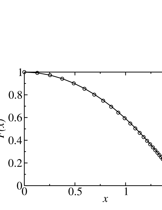
Figure 4: Plot of our numerical data (open circles) and fit to our interpolation formula $F(x)$ (straight line) as given by Eq. (34).

of our numerical data to the interpolation formula

$$m_{v}=\frac{0.03627a_{v}^{2}\hbar^{2}}{\rho_{s}u_{\text{rms}}^{4}}F(x),$$ (33)

where $a_{v}$ is the separation between nearest neighbor vortices, $x\equiv|\alpha|du_{\text{rms}}^{2}/\hbar$, and

$$F(x)\approx 1-0.4099x^{2}\;.$$ (34)

The above fit is motivated by a simple analytic calculation in which the two modes $\omega_{1,2}({\bf q})$ are replaced by their long-wavelength approximations (see Appendix B for details). Eq. (34) holds only as long as the r.h.s. is positive, while $F(x)=0$ for larger $x$ (we will see below and in Fig. 5 that this apparent upper bound on $x$ is relaxed once we allow for viscous damping). Similarly, for the frequency $\omega_{mp}$ in Fig. 3, we obtain $\omega_{mp}=\sqrt{\omega_{p}^{2}+\omega_{c}^{2}}$ with

$$\omega_{p}=\frac{35.45\rho_{s}u_{\text{rms}}^{2}}{\hbar a_{v}^{2}[F(x)]^{1/2}}~{}~{};~{}~{}\omega_{c}=\frac{27.57\rho_{s}u_{\text{rms}}^{2}xF(x)}{\hbar a_{v}^{2}}.$$ (35)

For the experiments of Ref. [1] we estimate $\rho_{s}=12$ meV [29], $u_{\text{rms}}=20$ Å [30], $a=3.83$ Å, and $a_{v}=240$ Å. The overall scale for $m_{v}$ is determined by setting $n_{S}=n_{MI}$ so that $x=0$ and $F(x)=1$. This yields $m_{v}\approx 8m_{e}$ and $\hbar\omega_{p}\approx 3$ meV (or $\nu_{p}\approx 0.7$ THz). For a more accurate determination, we need $n_{S}$, for which there is considerable uncertainty e.g. for $|n_{S}-n_{MI}|=0.015$, we find $x=1.29$, $m_{v}\approx 3m_{e}$ and $\hbar\omega_{p}\approx 5$ meV.

5 Limitations

We now consider the influence of a variety of effects which have been neglected in the computation of Section 4. The extensions were already discussed in Section 3, and here we will make quantitative estimates.

5.1 Viscous drag

It is conventional in models of vortex dynamics at low frequencies [31] to include a dissipative viscous drag term in the equations of motion, contributing an additional force

$${\bf F}_{D}(j)=-\eta d\frac{d{\bf r}_{j}}{dt},$$ (36)

to the r.h.s. of Eq. (2). This leads to the transformation Eq. (27) in the dynamical matrix. There are no reliable theoretical estimates for the viscous drag co-efficient, $\eta$, for the cuprates. However, we can obtain estimates of its value from measurements of the Hall angle, $\theta_{H}$, which is given by [31, 32] $\tan\theta_{H}=\alpha/\eta$. Harris et al. [32] observed a dramatic increase in the value $|\tan\theta_{H}|$, to the value 0.85, at low $T$ in “60 K” YBa₂Cu₃O_6+y crystals, suggesting a small $\eta$, and weak dissipation in vortex motion. For our purposes, we need the value of $\eta$ for frequencies of order $\omega_{p}$, and not just in the d.c. limit. The very naïve expectation that $\eta(\omega)$ behaves like the quasiparticle microwave conductivity would suggest it decreases rapidly beyond a few tens of GHz, well below $\omega_{p}$ [33]. Lacking solid information, we will be satisfied with an estimate of the influence of viscous drag obtained by neglecting the frequency dependence of $\eta$ (a probable overestimate of its influence). The resulting corrections to Eqs. (33-35) are easily obtained (as in Ref. [11]), and can be represented by the replacement

$$F(x)\rightarrow F(x,y),~{}\mbox{where}~{}y\equiv\frac{\eta du_{\text{rms}}^{2}}{\hbar}$$ (37)

and

$$F(x,0)=F(x).$$ (38)

The sketch of the function $F(x,y)$ is in Fig. 5; as long as $y>0$, we have $F(x,y)>0$.

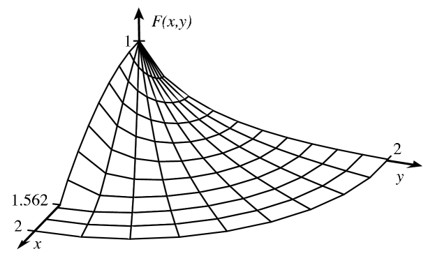
Figure 5: Plot of the function $F(x,y)$ which replaces $F(x)$ in Eqs. (33,34,35) upon including viscous drag, $\eta$ ($y\equiv\eta du_{\rm rms}^{2}/\hbar$). The argument $x$ measures the Hall drag $\alpha$ ($x\equiv|\alpha|du_{\rm rms}^{2}/\hbar$) and the Hall angle is determined by $|\tan\theta_{H}|=x/y$.

As expected, the viscous damping decreases the estimate of the mass, and this decrease is exponential for large $y$, e.g. at $x=0$ we have the interpolation formula

$$F(0,y)\approx(1+0.41y+2.69y^{2})e^{-3.43y}.$$ (39)

5.2 Meissner screening

The interaction in Eq. (3) is screened at long distances by the supercurrents, and the intervortex coupling becomes exponentially small. This does have an important influence at small momenta in that the shear mode of the vortex lattice disperses as [22, 23] $\sim q^{2}$. However, as long as $a_{v}\ll\lambda$, there will not be a significant influence on $u_{\text{rms}}$ or $\omega_{p}$.

5.3 Retardation

The interaction Eq. (3) is assumed to be instantaneous; in reality it is retarded by the propagation of the charged plasmon mode of the superfluid, and these effects were included in Eqs. (26) and (31). We can estimate the corrections due to this mode in a model of superfluid layers coupled by the long-range Coulomb interaction. In physical terms, we compare the energy per unit area of a ‘phase fluctuation’ at the wavevector of the vortex lattice Brillouin zone boundary ($\sim\rho_{s}/a_{v}^{2}$) with its electrostatic energy ($\sim\hbar^{2}\omega_{p}^{2}/(e^{2}d)$); this shows that such corrections are of relative order $\sim(\hbar^{2}/m_{v})/(e^{2}d)$. Alternatively this ratio can be viewed as the order of magnitude of the two terms in the denominator of the fourth term in Eq. (31). For the parameters above and $d=7.5$ Å this ratio is $\sim 0.009$, and hence quite small.

5.4 Nodal quasiparticles

We expect that nodal quasiparticles contribute to the viscous drag, and so their contribution was already included in the experimentally determined estimate of $\eta$ in (i). The nodal quasiparticle contribution to $m_{v}$ and $\eta$ has recently been discussed at some length in Ref. [34]. This analysis finds an infrared finite correction to $m_{v}$, and a contribution to $\eta$ which vanishes as $T\rightarrow 0$. The latter observations are consistent with the observations of Harris et al. [32].

5.5 Disorder

We have assumed here a triangular lattice of vortices. In reality, STM experiments show significant deviations from such a structure, presumably because of an appreciable random pinning potential. This pinning potential will also modify the vortex oscillation frequencies and its mean square displacement. Both pinning and damping $\eta$ tend to reduce vortex motion. For this reason, the estimates of $m_{v}$ above in which these effects are neglected must be regarded as upper bounds.

The above considerations make it clear that new experiments on cleaner underdoped samples, along with a determination of the spatial dependence of the hole density (to specify $\alpha$), are necessary to obtain a more precise value for $m_{v}$; determining the $H$ dependence of $m_{v}$ will enable confrontation with theory.

6 Implications

An important consequence of our theory is the emergence of $\omega_{p}$ as a characteristic frequency of the vortex dynamics. It would therefore be valuable to have an inelastic scattering probe which can explore energy transfer on the scale of $\hbar\omega_{p}$, and with momentum transfer on the scale of $h/a_{v}$, possibly by neutron [35] or X-ray scattering; observation of a resonance at such wavevectors and frequencies, along with its magnetic field dependence, could provide a direct signal of the quantum zero-point motion of the vortices. A direct theoretical consideration of magnetoconductivity in our picture would have implications for far-infrared or THz spectroscopy, allowing comparison to existing experiments [36]; further such experiments on more underdoped samples would also be of interest.

Another possibility is that the zero point motion of the vortices emerges in the spectrum of the LDOS measured by STM at an energy of order $\hbar\omega_{p}$. We speculate that understanding the ‘vortex core states’ observed in STM studies [2, 3] will require accounting for the quantum zero point motion of the vortices; it is intriguing that the measured energy of these states is quite close to our estimates of $\hbar\omega_{p}$.

7 Acknowledgements

We thank J. Brewer, E. Demler, Ø. Fischer, M. P. A. Fisher, W. Hardy, B. Keimer, N. P. Ong, T. Senthil, G. Sawatzky, Z. Tešanović and especially J. E. Hoffman and J. C. Seamus Davis for useful discussions. This research was supported by the NSF under grants DMR-0457440 (L. Balents), DMR-0098226 and DMR-0455678 (S.S.), the Packard Foundation (L. Balents), the Deutsche Forschungsgemeinschaft under grant BA 2263/1-1 (L. Bartosch), and the John Simon Guggenheim Memorial Foundation (S.S.).

Appendix A Evaluation of ‘magnetophonon’ modes

In this appendix we show how the ‘phonon’ and ‘magnetophonon’ modes as depicted in Figs. 2 and 3 can be calculated using the well-known Ewald summation technique (see e.g. Ref. [37]). Our calculation is similar to existing calculations and we will make contact with earlier work by considering a generalized potential energy of the form

$$U=\frac{g^{2}}{2}\sum_{i\neq k}\frac{1}{p|{\bf r}_{i}-{\bf r}_{k}|^{p}}\;,$$ (40)

with $p>0$. Here, ${\bf r}_{i}$ is the position of the $i$’th ‘charge’ (which could also be a real charge) and denoting ${\bf R}_{i}$ as is its equilibrium position we write ${\bf r}_{i}={\bf R}_{i}+{\bf u}_{i}$. To minimize the total potential energy the ${\bf R}_{i}$ form a triangular Bravais lattice. For $p=1$, $U$ reduces to the potential energy of a two-dimensional Wigner crystal with charges interacting via the three-dimensional Coulomb interaction. We are particularly interested in the case $p\to 0$ where the interaction between ‘charges’ becomes logarithmic. This case applies to our vortex lattice: Taking the gradient of $U$ with respect to ${\bf r_{j}}$, we obtain the ‘electric’ force ${\bf F}_{E}(j)=-{\bf\nabla}_{{\bf r}_{j}}U$ on the $j$’th vortex from

$${\bf F}_{E}(j)=g^{2}\sum_{k(\neq j)}\frac{{\bf r}_{j}-{\bf r}_{k}}{|{\bf r}_{j}-{\bf r}_{k}|^{p+2}}$$ (41)

after setting $p=0$. Identifying $g^{2}=2\pi\rho_{s}$, this equation clearly reduces to Eq. (3).

By considering arbitrary $p$ we will now generalize a calculation by Bonsall and Maradudin [28]. First, we expand $U$ in the displacements from the equilibrium positions $u_{i\alpha}$ (with $\alpha=x,y$ labeling the two cartesian coordinates) and only keep terms up to second order,

$$U=U_{0}+\frac{m_{v}}{2}\sum_{i\alpha j\beta}\Omega^{2}_{i\alpha;j\beta}\,u_{i\alpha}u_{j\beta}\;.$$ (42)

To determine the normal modes we essentially have to diagonalize the matrix

$$\Omega^{2}_{i\alpha;j\beta}\equiv\frac{1}{m_{v}}\left(\frac{\partial^{2}}{\partial u_{i\alpha}u_{j\beta}}U\right)_{{\bf u}=0}\;.$$ (43)

Fourier transforming $\Omega^{2}_{i\alpha;j\beta}$ to momentum space gives us a block-diagonal matrix $\Omega^{2}_{\alpha\beta}({\bf q})$ where each block is a $2\times 2$ matrix. The action for the vortices is then given by Eq. (24) with the dynamical matrix

$$D_{\alpha\beta}({\bf q},\omega)=A_{0}m_{v}\omega^{2}\delta_{\alpha\beta}+A_{0}B\omega\epsilon_{\alpha\beta}+A_{0}m_{v}\Omega_{\alpha\beta}^{2}({\bf q})\;.$$ (44)

Due to the long-range interaction all matrix elements $\Omega_{\alpha\beta}^{2}({\bf q})$ are slowly converging sums which we evaluate using the Ewald summation technique [37].

Let us write $\Omega^{2}_{\alpha\beta}({\bf q})$ as

$$\Omega^{2}_{\alpha\beta}({\bf q})=-\frac{g^{2}}{m_{v}}\left[S_{\alpha\beta}({\bf q})-S_{\alpha\beta}(0)\right]\;,$$ (45)

where the matrix elements $S_{\alpha\beta}({\bf q})$ are defined as

$$S_{\alpha\beta}({\bf q})=\frac{\partial^{2}}{\partial x_{\alpha}\partial x_{\beta}}\left.\sum_{{\bf R}_{j}\neq 0}\frac{e^{-i{\bf q}\cdot{\bf R}_{j}}}{p|{\bf x}-{\bf R}_{j}|^{p}}\right|_{{\bf x}=0}\;.$$ (46)

We can now use the integral representation

$$\frac{1}{py^{p}}=\frac{\epsilon^{p/2}}{2\Gamma(1+p/2)}\int_{0}^{\infty}dt\,t^{p/2-1}\,e^{-y^{2}\epsilon t}\;,$$ (47)

(with arbitrary $\epsilon>0$) and divide the integral on the r.h.s. in one part with $0<t<1$ and one part with $t>1$. Setting $y=|{\bf x}-{\bf R}_{j}|$ we see that the sum over the ${\bf R}_{j}$ in the integral from $1$ to infinity converges rapidly. The usual trick is to use Ewald’s generalized theta function transformation

$$\sum_{{\bf R}_{j}}e^{-i{\bf q}\cdot{\bf R}_{j}-|{\bf x}-{\bf R}_{j}|^{2}\epsilon t}=\frac{\pi}{A_{0}\epsilon t}\sum_{\bf G}e^{i({\bf G}+{\bf q})\cdot{\bf x}-{|{\bf G}+{\bf q}|^{2}}/{4\epsilon t}}\;,$$ (48)

and transform the integrand of the integral from $0$ to $1$ to a sum over the reciprocal lattice ${\bf G}$ such that this sum also converges rapidly. We then obtain

$$S_{\alpha\beta}({\bf q})=\, \frac{\epsilon^{p/2}}{2\Gamma(1+p/2)}\biggl{[}\sum_{{\bf R}_{j}}e^{-i{\bf q}\cdot{\bf R}_{j}}\left(4\epsilon^{2}R_{j\alpha}R_{j\beta}\varphi_{1+p/2}({\bf R}_{j}^{2}\epsilon)-2\epsilon\delta_{\alpha,\beta}\varphi_{p/2}({\bf R}_{j}^{2}\epsilon)\right)$$

$$\ +\frac{4\epsilon\delta_{\alpha,\beta}}{2+p}-\frac{\pi}{A_{0}\epsilon}\sum_{\bf G}(q_{\alpha}+G_{\alpha})(q_{\beta}+G_{\beta})\varphi_{-p/2}(|{\bf q}+{\bf G}|^{2}/4\epsilon)\biggr{]}\;,$$ (49)

where

$$\varphi_{\nu}(z)=\int_{1}^{\infty}dt\,t^{\nu}e^{-zt}$$ (50)

is a Misra function. The matrix $\Omega_{\alpha\beta}^{2}({\bf q})$ is now given by

$$\Omega_{\alpha\beta}^{2}({\bf q})=\, \frac{g^{2}\pi\epsilon^{p/2-1}}{2\Gamma(1+p/2)m_{v}A_{0}}\biggl{[}\sum_{\bf G}(q_{\alpha}+G_{\alpha})(q_{\beta}+G_{\beta})\varphi_{-p/2}(|{\bf q}+{\bf G}|^{2}/4\epsilon)$$

$$\qquad\qquad-\sum_{{\bf G}\neq 0}G_{\alpha}G_{\beta}\,\varphi_{-p/2}({\bf G}^{2}/4\epsilon)\biggr{]}$$

$${}+\, \frac{g^{2}\epsilon^{p/2}}{2\Gamma(1+p/2)m_{v}}\sum_{{\bf R}_{j}}\left[1-\cos({\bf q}\cdot{\bf R}_{j})\right][4\epsilon^{2}R_{j\alpha}R_{j\beta}\,\varphi_{1+p/2}({\bf R}_{j}^{2}\epsilon)$$

$$\qquad\qquad{}-2\epsilon\delta_{\alpha,\beta}\varphi_{p/2}({\bf R}_{j}^{2}\epsilon)]\;.$$ (51)

Setting $p=1$ we recover Eq. (3.10) of Ref. [28] as we should expect. The case $p\to 0$ is of interest to us. For our vortex lattice we have $g^{2}=2\pi\rho_{s}$. Using

$$\varphi_{0}(z)=\, \frac{1}{z}\,e^{-z}\;,$$ (52)

$$\varphi_{1}(z)=\, \left(1+\frac{1}{z}\right)\frac{1}{z}\,e^{-z}\;,$$ (53)

we see that when letting $\epsilon\to 0$ our dynamical matrix evaluated here agrees with the dynamical matrix given in Eq. (26) if we neglect retardation effects. We can now go ahead and calculate the ‘phonon’ or ‘magnetophonon’ dispersion using

$$\omega_{1,2}^{2}=\frac{(\Omega_{11}^{2}+\Omega_{22}^{2}+\omega_{c}^{2})}{2}\mp\sqrt{\frac{({\Omega_{11}^{2}+\Omega_{22}^{2}+\omega_{c}^{2}})^{2}}{4}-\Omega_{11}^{2}\Omega_{22}^{2}+\Omega_{12}^{2}\Omega_{21}^{2}}\;.$$ (54)

Here $\omega_{c}=B/m_{v}=\pi(n_{s}-n_{MI})/a^{2}m_{v}$ is the ‘cyclotron’ frequency. Identifying the plasma frequency

$$\omega_{p}=\left(\frac{2\pi g^{2}}{m_{v}A_{0}}\right)^{1/2}$$ (55)

as the characteristic frequency we can evaluate $\omega_{1}({\bf q})$ and $\omega_{2}({\bf q})$ using Eq. (51). It turns out that the sums over ${\bf R}_{j}$ and ${\bf G}$ indeed converge rapidly and that $\omega_{1,2}({\bf q})$ are indeed independent of the value of $\epsilon$. A plot of the spectrum for $n_{s}=n_{MI}$ (zero ‘magnetic’ field $B$) is shown in Fig. 2. Turning on the ‘magnetic’ field $B$ leads to an avoided crossing of the two modes. This can be seen in Fig. 3 where we have chosen $\omega_{c}=0.5\,\omega_{p}$.

Finally we would like to note that in the long-wave length limit the spectrum becomes isotopic and we find (with $a_{v}$ being the distance between nearest neighbor vortices)

$$\omega_{1}({\bf q}) \sim\frac{3^{1/4}}{\sqrt{32\pi}}\,\frac{\omega_{p}^{2}}{\omega_{mp}}\,(a_{v}q)\;,$$ (56)

$$\omega_{2}({\bf q}) \sim\omega_{mp}\;,$$ (57)

where $\omega_{mp}=\sqrt{\omega_{p}^{2}+\omega_{c}^{2}}$ is the ‘magnetophonon’ frequency. With or without the ‘magnetic’ field the shear mode is always linear in $q$.

Appendix B Simple Debye model and beyond

It is instructive to evaluate $u_{\text{rms}}^{2}$ in the Debye approximation where we replace $\omega_{1}({\bf q})$ and $\omega_{2}({\bf q})$ by Eqs. (56) and (57). Also, as usual we replace the first Brillouin zone by a Debye sphere of the same volume. Using Eq. (32) we obtain in this approximation

$$u_{\text{rms}}^{2}=(5/2)\,\hbar/2m_{v}\omega_{mp}\;,$$ (58)

which for $B=0$ simplifies to $u_{\text{rms}}^{2}=(5/2)\,\hbar/2m_{v}\omega_{p}$. To this the shear mode $\omega_{1}({\bf q})$ contributes 80%. Solving for the inertial mass of the vortex we now obtain

$$m_{v}=\frac{25\sqrt{3}\,\hbar^{2}a_{0}^{2}}{128\pi^{2}\rho_{s}u_{\text{rms}}^{4}}-\frac{\sqrt{3}a_{0}^{2}B^{2}}{4\pi^{2}\rho_{s}}\;.$$ (59)

More accurately, we can evaluate the integral in Eq. (32) for the exact dispersion relation numerically. Extracting the zero field result we have

$$u_{\text{rms}}^{2}=2.5718\cdot\frac{\hbar}{2m_{v}\omega_{p}}\,I(B/m_{v}\omega_{p})\;,$$ (60)

with $I(0)=1$. The numerically determined prefactor $2.5718$ corresponds to the factor $5/2$ in the Debye approximation. The small deviation is mainly due to the fact that as can be seen in Fig. 2 both $\omega_{1}({\bf q})$ and $\omega_{2}({\bf q})$ are on average slightly overestimated by Eqs. (56) and (57). Solving for the mass of a vortex we find

$$m_{v}=\frac{(2.5718)^{2}\sqrt{3}\,\hbar^{2}a_{0}^{2}}{32\pi^{2}\rho_{s}u_{\text{rms}}^{4}}\,F(u_{\text{rms}}^{2}B/\hbar)\;.$$ (61)

If we define $I_{2}(z)\equiv z^{1/2}I(z^{1/2})/2$ then the normalized function $F$ is related to the inverse of $I_{2}$ by $F(x)=x^{2}/4I_{2}^{-1}(x)$ and satisfies $F(0)=1$. While for the case of the exact dispersion relation considered here $F(x)$ has to be calculated numerically, Eq. (59) suggests a fit of the form $F(x)=1-c_{1}x^{2}$. As can be seen in Fig. 4 the quality of such a fit turns out to be excellent.

References

- [1] J. E. Hoffman, E. W. Hudson, K. M. Lang, V. Madhavan, S. H. Pan, H. Eisaki, S. Uchida, and J. C. Davis, Science 295, 466 (2002).
- [2] B. W. Hoogenboom, K. Kadowaki, B. Revaz, M. Li, Ch. Renner, and Ø. Fischer, Phys. Rev. Lett. 87, 267001 (2001); G. Levy, M. Kugler, A. A. Manuel, Ø. Fischer, and M. Li, Phys. Rev. Lett. 95, 257005 (2005).
- [3] S. H. Pan, E. W. Hudson, A. K. Gupta, K.-W. Ng, H. Eisaki, S. Uchida, and J. C. Davis, Phys. Rev. Lett. 85, 1536 (2000).
- [4] L. Balents, L. Bartosch, A. Burkov, S. Sachdev, and K. Sengupta, Phys. Rev. B 71, 144508 (2005).
- [5] L. Balents, L. Bartosch, A. Burkov, S. Sachdev, and K. Sengupta, Phys. Rev. B 71, 144509 (2005).
- [6] Z. Tešanović, Phys. Rev. Lett. 93, 217004 (2004); M. Franz, D. E. Sheehy, and Z. Tešanović, Phys. Rev. Lett. 88, 257005 (2002).
- [7] J. M. Tranquada, B. J. Sternlieb, J. D. Axe, Y. Nakamura, and S. Uchida, Nature 375, 561 (1995); J. M. Tranquada, H. Woo, T. G. Perring, H. Goka, G. D. Gu, G. Xu, M. Fujita, and K. Yamada, Nature 429, 534 (2004).
- [8] The LDOS modulations are a signal of valence-bond-solid (VBS) order that can be associated with the vortex flavors [4] (see also C. Lannert, M. P. A. Fisher, and T. Senthil, Phys. Rev. B 63, 134510 (2001)). VBS order in vortex cores was predicted in K. Park and S. Sachdev, Phys. Rev. B 64, 184510 (2001).
- [9] G. E. Volovik, Pisma Zh. Eksp. Teor. Fiz. 65 201 (1997) [JETP Lett. 65 217 (1997)].
- [10] N. B. Kopnin, Theory of Nonequilibrium Superconductivity, Cambridge University Press, Cambridge (2001); N. B. Kopnin and V. M. Vinokur, Phys. Rev. Lett. 81, 3952 (1998).
- [11] G. Blatter, V. B. Geshkenbein, and V. M. Vinokur, Phys. Rev. Lett. 66, 3297 (1991); G. Blatter and B. Ivlev, Phys. Rev. Lett. 70, 2621 (1993).
- [12] J.-M. Duan and A. J. Leggett, Phys. Rev. Lett. 68, 1216 (1992).
- [13] D. M. Gaitonde and T. V. Ramakrishnan, Phys. Rev. B 56, 11951 (1997).
- [14] M. W. Coffey, J. Phys. A 31, 6103 (1998).
- [15] J. H. Han, J. S. Kim, M. J. Kim, and P. Ao, Phys. Rev. B 71, 125108 (2005).
- [16] F. D. M. Haldane and Y.-S. Wu, Phys. Rev. Lett. 55, 2887 (1985); P. Ao and D. J. Thouless, Phys. Rev. Lett. 70, 2158 (1993).
- [17] The long-range force in Eq. (3) requires that boundary conditions be chosen carefully. In the dual charge analogy, we need a uniform neutralizing background charge, and this contributes an additional force to Eq. (3), where is the area per vortex.
- [18] At , the vortex degeneracy is in the short-range pairing models of Ref. [5]. In Ref. [21] we show that a similar degeneracy can be understood in long-range pairing models of -wave superconductors based upon the gauge theory of X.-G. Wen and P. A. Lee, Phys. Rev. Lett. 76, 503 (1996). Any distinctions between these cases have no impact on the considerations of the present paper.
- [19] J. M. Harris, N. P. Ong, P. Matl, R. Gagnon, L. Taillefer, T. Kimura, and K. Kitazawa, Phys. Rev. B 51, R12053 (1995).
- [20] N. B. Kopnin and V. E. Kravtsov, Pis’ma Zh. Eksp. Teor. Fiz. 23, 631 (1976) [JETP Lett. 23, 578 (1976)].
- [21] L. Balents and S. Sachdev, to appear.
- [22] P. G. de Gennes and J. Matricon, Rev. Mod. Phys. 36, 45 (1964).
- [23] A. L. Fetter, P. C. Hohenberg, and P. Pincus, Phys. Rev. 147, 140 (1966); A. L. Fetter, Phys. Rev. 163, 390 (1967).
- [24] A. L. Fetter, Phys. Rev. 162, 143 (1967).
- [25] V. K. Tkachenko, Zh. Eksp. Teor. Fiz. 49, 1875 (1965) [Sov. Phys. JETP 22, 1282 (1966)].
- [26] G. Baym, Phys. Rev. B 51, 11697 (1995); Phys. Rev. Lett. 91, 110402 (2003).
- [27] H. Fukuyama, Sol. State. Comm. 17, 1323 (1975).
- [28] L. Bonsall and A. A. Maradudin, Phys. Rev. B 15, 1959 (1977).
- [29] M. Weber, A. Amato, F. N. Gygax, A. Schenck, H. Maletta, V. N. Duginov, V. G. Grebinnik, A. B. Lazarev, V. G. Olshevsky, V. Yu. Pomjakushin, S. N. Shilov, V. A. Zhukov, B. F. Kirillov, A. V. Pirogov, A. N. Ponomarev, V. G. Storchak, S. Kapusta, and J. Bock, Phys. Rev. B 48, 13022 (1993).
- [30] We estimate from the published data in Ref. [1]. Also, using the correspondence between the LDOS modulations and the vortex core states [2], we obtain a similar number from the measurements of Ref. [3].
- [31] J. Bardeen and M. J. Stephen, Phys. Rev. 140, A1197 (1965); P. Nozières and W. F. Vinen, Philos. Mag. 14, 667 (1966).
- [32] J. M. Harris, Y. F. Yan, O. K. C. Tsui, Y. Matsuda, and N. P. Ong, Phys. Rev. Lett. 73, 1711 (1994).
- [33] P. J. Turner, R. Harris, S. Kamal, M. E. Hayden, D. M. Broun, D. C. Morgan, A. Hosseini, P. Dosanjh, G. K. Mullins, J. S. Preston, R. Liang, D. A. Bonn, and W. N. Hardy, Phys. Rev. Lett. 90, 237005 (2003).
- [34] P. Nikolić and S. Sachdev, cond-mat/0511298.
- [35] B. Keimer, W. Y. Shih, R. W. Erwin, J. W. Lynn, F. Dogan, and I. A. Aksay, Phys. Rev. Lett. 73, 3459 (1994).
- [36] H.-T. S. Lihn, S. Wu, H. D. Drew, S. Kaplan, Qi Li, and D. B. Fenner, Phys. Rev. Lett. 76, 3810 (1996) and references therein.
- [37] J. M. Ziman, Principles of the Theory of Solids Cambridge University Press, Cambridge (1964).