Field dependence of the magnetic spectrum in anisotropic and Dzyaloshinskii-Moriya antiferromagnets: I. Theory

Abstract

We consider theoretically the effects of an applied uniform magnetic field on the magnetic spectrum of anisotropic two-dimensional and Dzyaloshinskii-Moriya layered quantum Heisenberg antiferromagnets. The former case is relevant for systems such as the two-dimensional square lattice antiferromagnet Sr₂CuO₂Cl₂, while the latter is known to be relevant to the physics of the layered orthorhombic antiferromagnet La₂CuO₄. We first establish the correspondence between the low-energy spectrum obtained within the anisotropic non-linear sigma model and by means of the spin-wave approximation for a standard easy-axis antiferromagent. Then, we focus on the field-theory approach to calculate the magnetic-field dependence of the magnon gaps and spectral intensities for magnetic fields applied along the three possible crystallographic directions. We discuss the various possible ground states and their evolution with temperature for the different field orientations, and the occurrence of spin-flop transitions for fields perpendicular to the layers (transverse fields) as well as for fields along the easy axis (longitudinal fields). Measurements of the one-magnon Raman spectrum in Sr₂CuO₂Cl₂ and La₂CuO₄ and a comparison between the experimental results and the predictions of the present theory will be reported in part II of this research work [L. Benfatto et al., forthcoming article, cond-mat/0602664].

I Introduction

The relevance of antisymmetric superexchange interactions in spin Hamiltonians describing quantum antiferromagnetic (AF) systems has been acknowledged long ago by Dzyaloshinskii.D Soon after, Moriya showed that such interactions arise naturally in perturbation theory due to the spin-orbit coupling in magnetic systems with low symmetry.M Nowadays, a number of AF systems are known to belong to the class of Dzyaloshinskii-Moriya (DM) magnets, such as $\alpha$-Fe₂O₃, LaMnO₃,Talbayev and K₂V₃O₈,Lumsden and to exhibit unusual and interesting magnetic properties in the presence of quantum fluctuations and/or applied magnetic field.Talbayev ; Kotov ; sasha

Also belonging to the class of DM antiferromagnets is La₂CuO₄, which is a parent compound of high-temperature superconductors. In La₂CuO₄ the unique combination of antisymmetric superexchange, caused by the staggered tilting pattern of oxygen octahedra around each copper ion in the low-temperature orthorhombic (LTO) phase, and weak interlayer coupling, results in an interesting four sublattice structure for the antiferromagnetism of La₂CuO₄, where the Cu⁺⁺ spins are canted out of the CuO₂ layers with opposite canting directions between neighboring layers.Shekhtman ; Thio ; Thio90 ; Papanicolaou These small ferromagnetic moments lead to a quite unconventional physics in the antiferromagentic phase. For example, when a small magnetic field is applied perpendicular to the layers the magnetic susceptibility shows a strong enhancement as the Neél temperature is approached, due to the formation of these ferromagnetic moments.Thio ; MLVC ; Gooding . When the field strenght is further enhanced one can observe a spin flop of the ferromagnetic moments whith respect to the out-of-plane staggered order that they display at zero field. Thio ; Ando-Mag-Anisotropy ; Papanicolaou Analogously the spin-flop transition of the staggered in-plane AF moments for a field along the easy axis is accompanied by new effects related to the presence of the DM interaction. Thio90 ; Papanicolaou Recently new theoretical approaches have been proposed MLVC ; Gooding ; Raman to integrate the semiclassical picture already presented in the prior work of Refs. [Shekhtman, ; Thio, ; Thio90, ; Papanicolaou, ]. Even thought the basic physical picture remains the same, the inclusion of quantum effects in the long-wavelenght formulation of the spin problem discussed in Ref. [MLVC, ; Raman, ] allowed for a straightforward and complete understanding of the unusual magnetic-susceptibility anisotropies observed in La₂CuO₄ for a rather large temperature range, $0<T<400$ K. Moreover, a particular attention has been devoted in Ref. [Raman, ] to the analysis of the one-magnon excitations by means of Raman spectroscopy, and the use of the long-wavelength theory turns out to be very convenient to understand why the DM interaction is behind the appearanceGozar of a field-induced mode for an in-plane magnetic field.Raman

A better understanding of the anomalies related to the presence of the DM interaction in La₂CuO₄ compounds can be achieved by directly comparing its properties with those of a similar spin system like Sr₂CuO₂Cl₂. In this case the DM interaction is absent due to the higher crystal symmetry, but spin-orbit coupling can still give rise to small anisotropies of purely quantum mechanical origin.yildrim Thus quantum corrections coming from spin-orbit coupling give rise to a quite small easy-axis anisotropy, so that a gap in the in-plane magnon excitations has been observed in ESR.ESR As a consequence, Sr₂CuO₂Cl₂ behaves as an ordinary easy-axis antiferromagnet, in contrast to La₂CuO₄ which should be classified as an unconventional easy-axis antiferromagnet.

It is the purpose of this article to study in detail the influence of an applied uniform magnetic field on the magnetic spectrum for the above two cases: anisotropic two-dimensional and layered DM antiferromagnets, and to compare the qualitative differences between these two cases. This will be done mainly using the continuum quantum field theory appropriate for each of these two cases, i.e. the non-linear sigma model (NLSM), properly modified to account for conventional or DM anisotropies. Nonetheless, we will sketch in the beginning the calculation of the magnon gaps within the framework of the semiclassical approximation for conventional antiferromagnets, and we demonstrate the complete equivalence between the two approaches as far as the gaps values at low temperature are concerned. However, as it will become clear in the following, the quantum NLSM followed here allows also to account for the quantum and thermal effects of the spin fluctuation, which were neglected in the previous approaches Thio ; Thio90 ; Papanicolaou . As a consequence, we can evaluate (within the given saddle-point approximation for the transverse spin fluctuations) the full $(H,T)$ phase diagram for a field in the various direction, which can be compared with the existing experimental data. At the same time, the continuum field theory provides an elegant and straighforward description of the spin fluctuations in the coupled-layers case, and also of the various spin-flop transitions that may occur in La₂CuO₄ at moderate fields.

The structure of the paper is as follows. In Section II we introduce the model Hamiltonians for Sr₂CuO₂Cl₂ and La₂CuO₄, appropriate to describe a conventional anisotropic two-dimensional antiferromagnet and a DM antiferromagnet, respectively. In Section III we sketch the standard semiclassical calculations of the magnon gaps at zero field in the two cases, and at finite magnetic field for the standard anisotropic case. Then the same (conventional) results are reproduced in Section IV using the NLSM approach, whose main properties are here described. Section V is dedicated to the case of a layered DM antiferromagnet, and the effects of an uniform magnetic field applied along the three crystallographic directions are extensively discussed, with reference to the specific structure of La₂CuO₄. The conclusions are reported in Section VI. In a second part,theo-exp we shall make a quantitative comparison between the predictions of the theory developed in this article and the magnetic spectrum probed by one-magnon Raman scattering in both La₂CuO₄ and Sr₂CuO₂Cl₂.

II Spin-Hamiltonians for conventional and DM anisotropies

La₂CuO₄ is a body centered orthorhombic antiferromagnet with $Bmab$ crystal structure. A single layer of CuO₂ ions in La₂CuO₄ can be described by the $S=1/2$ Hamiltonian

$$H_{sl}[{\bf S},{\bf D}]=J\sum_{\langle i,j\rangle}{\bf S}_{i}\cdot{\bf S}_{j}+\sum_{\langle i,j\rangle}{\bf D}_{ij}\cdot\left({\bf S}_{i}\times{\bf S}_{j}\right)+\sum_{\langle i,j\rangle}{\bf S}_{i}\cdot\overleftrightarrow{\bf\Gamma}_{ij}\cdot{\bf S}_{j},$$ (1)

where ${\bf D}_{ij}$ and $\overleftrightarrow{\bf\Gamma}_{ij}$ are, respectively, the DM and XY anisotropic interaction terms that arise due to the spin-orbit coupling and direct-exchange in the low-temperature orthorhombic (LTO) phase of La₂CuO₄.Shekhtman Throughout this work we adopt the LTO $(abc)$ coordinate system of Fig. 1,coord-system for both the spin and lattice degrees of freedom, and we use units where $\hbar=k_{B}=1$.

The direction and the alternating pattern of the DM vectors, shown in Fig. 1, have been calculated by several authors Shekhtman by taking into account the tilting structure of the oxygen octahedra and of the symmetry of the La₂CuO₄ crystal. For La₂CuO₄ the DM vectors are in good approximation perpendicular to the $Cu-Cu$ bonds and change sign from one bond to the next one:

$${\bf D}_{AB}=\frac{1}{\sqrt{2}}(d,-d,0),\quad{\bf D}_{AC}=\frac{1}{\sqrt{2}}(d,d,0),$$ (2)

while the $XY$ matrices $\overleftrightarrow{\Gamma}$ provide essentially an easy-plane anisotropy for the Hamiltonian (1):

$$\overleftrightarrow{\Gamma}_{AB}{=}\left(\begin{array}[]{ccc}\Gamma_{1}&\Gamma_{2}&0\\ \Gamma_{2}&\Gamma_{1}&0\\ 0&0&\Gamma_{3}\end{array}\right)\!\!,\;\overleftrightarrow{\Gamma}_{AC}{=}\left(\begin{array}[]{ccc}\Gamma_{1}&-\Gamma_{2}&0\\ -\Gamma_{2}&\Gamma_{1}&0\\ 0&0&\Gamma_{3}\end{array}\right)\!\!,$$ (9)

where $AB$ and $AC$ label the Cu⁺⁺ sites on horizontal/vertical bonds respectively (see Fig. 1). As it has been stressed by Shekhtman et al. Shekhtman , even though the parameters $d$ and $\Gamma_{1,2,3}>0$ have different orders of magnitude, with $d\sim 10^{-2}J$ and $\Gamma_{i}\sim 10^{-4}J$, they should be considered on the same footing (see also discussion following Eq. (19) below). Indeed, one can show that considering the two last terms of Eq. (1) the interaction between spins on a neighboring bond can be written in a completely isotropic form by rotating locally the spin operators around the ${\bf D}_{ij}$ axis by an angle $\theta_{ij}=\arctan|{\bf D}_{ij}|/2J$. As a consequence, weak ferromagnetism arises only when global frustration of the DM pattern exists. In term of the DM vectors defined above, this condition corresponds to having ${\bf d}_{+}\neq{\bf d}_{-}$, where ${\bf d}\pm=({\bf D}_{AB}\pm{\bf D}_{BC})/2$. This condition is clearly satisfied by the DM vectors (2), so that WF is expected in La₂CuO₄.

A realistic model for La₂CuO₄ should include also interlayer coupling. In the orthorhombic unit cell of La₂CuO₄ the spins of the $Cu$ atoms are displaced by an in-plane diagonal vector $(1/2,1/2,0)$ from one layer to the next one. As a consequence, given a couple of spins in a layer and the nearest couple in the next one, the DM vector of the corresponding bond will change sign. We can then write the full Hamiltonian as:

$$H=J_{\perp}\sum_{m}{\bf S}^{m}\cdot{\bf S}^{m+1}+\sum_{m}H_{sl}[{\bf S}^{m},{\bf D}^{m}],$$ (10)

where ${\bf S}^{m}$ represents the spin at a generic position $(i,j)$ of the $m$th plane and ${\bf D}^{m}_{AB,AC}=(-1)^{m}{\bf D}_{AB,AC}$. Since the La₂CuO₄ unit cell is body centered, the coupling $J_{\perp}$ in Eq. (10) connects the two spins at $(0,0,0)$ and $(1/2,0,1/2)$ in the LTO notation. It is worth noting that the pure 2D system (1) does not display any spin rotational symmetry, so it can order at finite temperature without violating the Mermin-Wagner theorem. However, in the presence of an interlayer coupling the transition to the AF state will ultimately have 3D character, with spins aligned AF also in the $c$ direction. On the other hand, as we shall discuss below, the interplay between the interlayer coupling and the DM interaction can lead to a quite unconventional behavior in the presence of a finite magnetic field. Indeed, the DM interaction is not only the source of an easy-plane anisotropy (the spins prefers to align perpendicularly to the DM vector ${\bf d}_{+}$), but induces also an anomalous coupling between the AF order parameter and an applied magnetic field.

These effects can be better understood by comparing the results obtained with the model (1) (and its three-dimensional version (10)) with the ones coming from a more conventional 2D anisotropic Heisenberg model, as:

$$H_{con}=\sum_{\langle i,j\rangle}JS_{i}^{b}S_{j}^{b}+(J-\alpha_{a})S_{i}^{a}S_{j}^{a}+(J-\alpha_{c})S_{i}^{c}S_{j}^{c}.$$ (11)

The Hamiltonian (11) is the appropriate starting model for Sr₂CuO₂Cl₂, where interlayer coupling is even less relevant than in La₂CuO₄ due to the frustation on the tetragonal unit cell. Here the crystallographic in-plane $a,b$ axes are choosen with $b$ parallel to the spin easy axis (which is along the $xy$ direction), so that we will have a similar notation to the one used for La₂CuO₄. However, $a=b$ for Sr₂CuO₂Cl₂, since the system is tetragonal. As we explained in the introduction, $\alpha_{a}$ should be zero in a tetragonal system. Nonetheless, quantum effects can induce an in-plane anisotropyyildrim which we will mimic with a finite $\alpha_{a}$ anisotropy term in what follows. To clarify to what extent the DM interaction introduces an anomalous behavior, we shall start our analysis of easy-axis antiferromagnetism from the anisotropic model (11). We will then be able to go back to the model (1)-(10) and to correctly distinguish the effects of the magnetic field alone from the ones arising from the presence of the DM interaction.

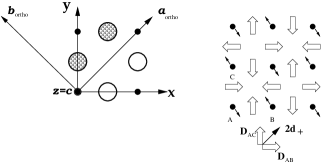
Figure 1: Left: the hatched circles represent the O^– ions tilted above the CuO₂ plane; the empty ones are tilted below it; small black circles are Cu⁺⁺ ions. Right: Schematic arrangement of the staggered magnetization (small arrows) and DM vectors (open arrows). Right bottom: definition of the vector ${\bf d}_{+}={\bf D}_{+}/4S$.

III Semiclassical approach

III.1 Conventional anisotropies

Let us start our analysis of the single-layer Hamiltonian (11) using a semiclassical approach. Similar calculations have been already carried out in different contexts, kittel ; Kubo and here we shall just review the main steps to fix the notation and to clarify the conventional behavior of an ordinary easy-axis antiferromagnet. Let us denote by ${\bf S}_{1}$ and ${\bf S}_{2}$ the spins on the two AF sublattices. The free energy density in the AF phase can be written:

$$F=zJS_{1}^{b}S_{2}^{b}+z(J-\alpha_{a})S_{1}^{a}S_{2}^{a}+z(J-\alpha_{c})S_{1}^{c}S_{2}^{c},$$ (12)

where $z$ is the number of nearest neighbors and $S^{a,b,c}$ are the components of the vector along the three crystallographic axes. Within the semiclassical approach, the spins are treated as classical vectors of length $S$: thus the ground-state configuration can be easily determined by imposing that $\nabla_{{\bf S}_{i}}F=0$. This condition clearly shows that the spins order along the $b$ direction, with ${\bf S}_{1}^{0}=-{\bf S}_{2}^{0}=S{\bf x}_{b}$. To calculate the magnon gaps one uses the classical equations of motion:

$$\frac{d{\bf S}_{i}}{dt}={\bf S}_{i}\times\nabla_{{\bf S}_{i}}F,\quad i=1,2$$ (13)

where $\nabla_{{\bf S}_{i}}F/(g_{s}\mu_{B})$ represents the effective local magnetic field around which each magnetic moment $(g_{s}\mu_{B}){\bf S}$ precesses. Here $g_{s}$ is the gyromagnetic ratio and $\mu_{B}$ is the Bohr magneton. By expanding the spins around the classical solution, ${\bf S}_{1}=S(m_{1}^{a},1,m_{1}^{b}),{\bf S}_{2}=S(m_{2}^{a},-1,m_{2}^{b})$ Eqs. (13) give a set of 4 coupled equations for the time dependence of the transverse spin fluctuations, which can be easily solved by putting $m_{i}^{\alpha}(t)=m_{i}^{\alpha}\exp(i\omega t)$. It then follows that the $\omega$ are the eigenvalues of the matrix (corresponding to the vector $(m_{1}^{c},m_{2}^{c},m_{1}^{a},m_{2}^{a})$):

$$izS\left(\begin{array}[]{cccc}0&0&J&J-\alpha_{c}\\ 0&0&-J+\alpha_{c}&-J\\ -J&-J+\alpha_{a}&0&0\\ J-\alpha_{a}&J&0&0\end{array}\right).$$ (14)

The eigenvalues $\omega=\pm\omega_{a}$ and $\omega=\pm\omega_{c}$ correspond to eigenmodes describing spin fluctuations with a larger $a/c$ component respectively, allowing for the identification of $\omega_{a}$ and $\omega_{c}$ as the magnon gaps for the in-plane and out-of-plane spin-wave modes:kittel

$$\omega_{a}=m_{a}=zS\sqrt{2\alpha_{a}J},\quad\omega_{c}=m_{c}=zS\sqrt{2\alpha_{c}J},$$ (15)

where we approximated $\sqrt{2\alpha_{a,c}J-\alpha_{a}\alpha_{c}}\approx\sqrt{2\alpha_{a,c}J}$ because $\alpha_{a},\alpha_{c}\ll J$.

In the presence of a finite magnetic field a term $-\sum_{i}{\bf H}\cdot{\bf S}_{i}$ must be added to Eq. (11), which translates into a term $-{\bf H}\cdot({\bf S}_{1}+{\bf S}_{2})$ in Eq. (12). Observe that in what follows we shall measure the magnetic field in units of $g_{s}\mu_{B}=1$, unless explicitly stated. Then one follows the same procedure as before, by noticing that when a transverse field is applied (i.e. a field perpendicular to the easy axis) the sublattice ground-state configurations ${\bf S}^{0}_{1,2}$ acquire an uniform component in the field direction proportional to $H/z(2J-\alpha_{a,c})$ (for a field along $a$ and $c$, respectively). By adding fluctuations transverse to the new equilibrium direction one finds for example for ${\bf H}\parallel a$ the fluctuation matrix:

$$izS\left(\begin{array}[]{cccc}0&0&J&J-\alpha_{c}\\ 0&0&-J+\alpha_{c}&-J\\ -J\cos^{2}\phi+(J-\alpha)\sin^{2}\phi-(H/zS)\sin\phi&J\sin^{2}\phi-(J-\alpha_{a})\cos^{2}\phi&0&0\\ -J\sin^{2}\phi+(J-\alpha)\cos^{2}\phi&J\cos^{2}\phi-(J-\alpha)\sin^{2}\phi+(H/zS)\sin\phi&0&0\end{array}\right),$$

where $\phi=\arcsin(H/zS(2J-\alpha_{a}))\approx H/zS2J$. As a consequence, the new magnon gaps are:Kubo

$$\omega_{a}(H)=\sqrt{m^{2}_{a}+H^{2}},\quad\omega_{c}(H)=m_{c}.$$ (16)

Observe that since the canting of the spins due to the magnetic field is small, the eigenmodes still describe fluctuations having predominantly $a$ or $c$ character, respectively. We see that the effect of a transverse magnetic field is to harden the gap of the mode in the field direction, and to leave the other gap unchanged. Indeed, when ${\bf H}$ is parallel to $c$ we find a similar result, with an increasing $\omega_{c}$ gap and a constant $\omega_{a}$ gap.

Finally, let us consider the case of a longitudinal field, i.e. of a field parallel to the easy axis. In this configuration no uniform spin magnetization develops, but the magnetic field effectively shifts the AF coupling along the easy axis in the two sublattices, so that the new fluctuation matrix reads:

$$izS\left(\begin{array}[]{cccc}0&0&J+H/zS&J-\alpha_{c}\\ 0&0&-J+\alpha_{c}&-(J-H/zS)\\ -(J+H/zS)&-J+\alpha_{a}&0&0\\ J-\alpha_{a}&J-H/zS&0&0\end{array}\right).$$

The four eigenvalues are given by

$${\omega^{2}}/{(zS)^{2}}=J(\alpha_{a}+\alpha_{c})-\alpha_{a}\alpha_{c}+(H/zS)^{2}\pm\sqrt{(\alpha_{c}-\alpha_{a})^{2}J^{2}+4(\alpha_{a}+\alpha_{c})J(H/zS)^{2}-(H/zS)^{2}(\alpha_{a}+\alpha_{c})^{2}},$$

and using the fact that $\alpha_{a},\alpha_{c}\ll J$ they can be readily expressed in terms of the bare gaps $m_{a},m_{c}$ as:

$${\omega_{a}^{2}}=\frac{m^{2}_{a}+m_{c}^{2}}{2}+H^{2}-\sqrt{\left(\frac{m^{2}_{a}-m_{c}^{2}}{2}\right)^{2}+4H^{2}\left(\frac{m^{2}_{c}+m_{a}^{2}}{2}\right)},$$

$${\omega_{c}^{2}}=\frac{m^{2}_{a}+m_{c}^{2}}{2}+H^{2}+\sqrt{\left(\frac{m^{2}_{a}-m_{c}^{2}}{2}\right)^{2}+4H^{2}\left(\frac{m^{2}_{c}+m_{a}^{2}}{2}\right)},$$ (17)

where we assumed $m_{c}>m_{a}$. Note that at fields larger than the bare gaps one observes essentially a linear increase of the magnon gaps with the magnetic field. In the case of degenerate gaps, $\alpha_{c}=\alpha_{a}$, only the linear regime is accessible and Eqs. (17) simplify to:kittel

$$\omega_{a}=m_{a}-H,\quad\omega_{c}=m_{c}+H.$$

III.2 Dzyaloshinskii-Moriya interactions

Let us discuss how the previous results are modified in the presence of DM interactions. First, taking into account that $\Gamma_{1,2}\ll d\ll J$ the free energy density corresponding to the Hamiltonian (1) can be written as:

$$F=zJ(S_{1}^{a}S_{2}^{a}+S_{1}^{b}S_{2}^{b})+z(J-\alpha_{c})S_{1}^{c}S_{2}^{c}+zd_{+}(S_{1}^{b}S_{2}^{c}-S_{1}^{c}S_{2}^{b}),$$

where $\alpha_{c}=\Gamma_{1}-\Gamma_{3}>0$ and $d_{+}=|{\bf d}_{+}|=d/\sqrt{2}$. The ground-state configuration of the previous free energy has been already discussed by several authors (see for example Shekhtman ; Thio ; Papanicolaou ). The spins order AF with an easy axis in the $b$ direction, but with an additional small ferromagnetic (FM) component along $c$, ${\bf S}_{1}^{0}=S(0,\cos\phi,\sin\phi)$ and ${\bf S}_{2}^{0}=S(0,-\cos\phi,\sin\phi)$. The angle $\phi$ of the out-of-plane canting of the spins is given by $\phi_{0}=(1/2)\arctan[2d_{+}/(2J-\alpha_{c})]\approx d_{+}/2J$ and it is due to the DM interaction (see also Fig. 3 below). When this canting is taken into account in the linearized equations of motion (13), one can easily see that the matrix for the transverse fluctuations in zero field has the same structure of Eq. (14), with

$$\alpha_{a}=d_{+}\phi_{0}\approx d_{+}^{2}/(2J).$$ (18)

As a consequence, the effect of the DM interaction is twofold: it induces the FM canting of the spins, and it reduces the AF coupling in the $a$ direction. The corresponding magnon gaps are, using Eq. (15) and the equivalence (18):

$$\omega_{a}=m_{a}=zSd_{+},\quad\omega_{c}=m_{c}=zS\sqrt{2\alpha_{c}J}.$$ (19)

Notice that the gap of the $a$ mode is proportional to $d$, while the gap of the $c$ mode scales with the square-root of the parameter $\alpha_{c}=\Gamma_{1}-\Gamma_{3}$. As a consequence, even though $\Gamma_{i}\sim 10^{-4}J$ and $d\sim 10^{-2}J$ the two gaps are of the same order of magnitude in La₂CuO₄. When a finite magnetic field is applied the system will evolve towards a new ground-state configuration. Following the procedure described above the new magnon gaps can be determined. However, we will not present these calculations here, because we shall describe in detail in the next sections how these results can be obtained using the NLSM approach, and how do they differ from the results (16) and (17), that we shall refer to as ’conventional’ in what follows.

IV NLSM formulation for conventional anisotropies

In this section we will show how the behavior of the spin gaps in the presence of magnetic field can be easily derived within a NLSM description of the low-energy physics of the spin model (11) and (10). We will first discuss the simple anisotropic model (11), to show the agreement with the results (16) and (17) presented above. Since the semiclassical approach is much more lengthly and less transparent than the NLSM description, we shall adopt the latter to deal with the more complicated case of the Hamiltonian (10).

The derivation of the NLSM starting for the 2D Heisenberg Hamiltonian has been extensively discussed in the literature.sachdev Here we just recall the main steps and stress the origin of the mass terms due to the anisotropies in Eq. (11). First, we decompose the unit vector ${\bf\Omega}_{i}={\bf S}_{i}/S$ at site ${\bf r}_{i}$ into its slowly-varying staggered and uniform components,

$${\bf\Omega}_{i}=\frac{{\bf S}_{i}(\tau)}{S}=e^{{\rm i}{\bf Q\cdot x}_{i}}{\bf n}({\bf x}_{i},\tau)+a{\bf L}({\bf x}_{i},\tau),$$ (20)

where ${\bf Q}=(\pi,\pi)$ and $a$ is the lattice parameter. The constraint ${\bf\Omega}^{2}_{i}=1$ is enforced by ${\bf n}^{2}_{i}=1$ and ${\bf L}_{i}\cdot{\bf n}_{i}=0$. Using this decomposition, the Heisenberg part of the Hamiltonian (1) has the standard form affleck

$${\cal L}_{HJ}=J\sum_{\langle i,j\rangle}{\bf S}_{i}\cdot{\bf S}_{j}=\frac{JS^{2}}{2}\int{\rm d}^{2}{\bf x}\left[(\nabla{\bf n})^{2}+8{\bf L}^{2}\right],$$ (21)

while the terms proportional to $\alpha_{a},\alpha_{c}$ give rise to:sces05

$${\cal L}_{\alpha}=-\sum_{\langle i,j\rangle}\alpha_{a}S_{i}^{a}S_{j}^{a}+\alpha_{c}S_{i}^{c}S_{j}^{c}=\frac{S^{2}}{a^{2}}\int{\rm d}^{2}{\bf x}\left[2\alpha_{a}n^{2}_{a}+2\alpha_{c}n^{2}_{c}+-\frac{1}{2}a^{2}\alpha_{a}(\nabla n_{\alpha})^{2}-\frac{1}{2}a^{2}\alpha_{c}(\nabla n_{c})^{2}\right].$$ (22)

Since $\alpha_{a,c}\ll J$ we can neglect the correction induced by the small anisotropies to the gradient of the transverse modes in Eq. (21), and we can retain just the first two terms of ${\cal L}_{\alpha}$. Using a path-integral coherent states representation of the spin states, which in addition to the previous contributions gives rise to the (dynamical) Wess-Zumino term affleck

$${\cal L}_{WZ}=\frac{-iS}{a}\int{\rm d}^{2}{\bf x}\,{\bf L}\cdot({\bf n}\times\dot{\bf n}),$$

we can obtain the partition function $Z=\int D{\bf n}\delta({\bf n}^{2}-1)e^{-{\mathcal{S}}}$, with the action ${\mathcal{S}}=\int{\rm d}\tau[{\cal L}_{HJ}+{\cal L}_{\alpha}+{\cal L}_{WZ}]$. After integration of the ${\bf L}$ fluctuations we obtain the following anisotropic non-linear $\sigma$ model ($\beta=1/T$ and $\int=\int_{0}^{\beta}{\rm d}\tau\int{\rm d}^{2}{\bf x}$):

$${\mathcal{S}}_{0}=\frac{1}{2gc}\int\left\{(\partial_{\tau}{\bf n})^{2}+c^{2}(\nabla{\bf n})^{2}+{m_{a}^{2}}{n}_{a}^{2}+m^{2}_{c}\;n_{c}^{2}\right\}.$$ (23)

The bare coupling constant $g$ and spin velocity $c$ are given by $gc=8Ja^{2}$ and $c=2\sqrt{2}JSa$, and we defined $m^{2}_{a,c}=32JS^{2}\alpha_{a,c}$, which corresponds to the result (15) above with $z=4$, as appropriate in two dimensions. In generic $d$ dimensions the coefficients $2\alpha_{a,c}$ in Eq. (22) are replaced by $z/2\alpha_{a,c}$ and one puts $gc=4dJa^{d}=2zJa^{d}$, leading again to the definition (15) of the masses. In the NLSM (23) the spin stiffness is renormalized by quantum fluctuations to $\rho_{s}=c(1/Ng-\Lambda/4\pi)$,sachdev ; CSY ; CHN where $\Lambda$ is a cutoff for momentum integrals and $N=3$ is the number of spin components. When the system orders we find the staggered magnetization at $\langle{\bf n}\rangle=\sigma_{0}\hat{\bf x}_{b}$, because the orientation along $\hat{\bf x}_{a}$ or $\hat{\bf x}_{c}$ would cost an energy $m_{a}$ or $m_{c}$, respectively.

It is worth noting that even though the NLSM (23) contains explicitly only the staggered spin component ${\bf n}$, nonetheless the saddle-point value of the uniform spin component ${\bf L}$ determined before integrating it out contains the residual information about the ferromagnetically ordered spin component. This is evident when an external magnetic field is applied on the system. In this case one can easily repeat the previous calculations by taking into account that the saddle-point value of the uniform magnetization ${\bf L}$ acquires an additional contribution proportional to ${\bf H}$:Loss

$${\bf L}=\frac{i}{8aSJ}({\bf n}\times\dot{\bf n})+\frac{1}{8aSJ}[{\bf H}-{\bf n}({\bf n}\cdot{\bf H})].$$ (24)

Observe that the first term is proportional to the time derivative of ${\bf n}$, so it averages to zero for the equlibrium configuration (indeed no FM component is present in the ordinary AF phase). However, at finite ${\bf H}$ a non-vanishing average uniform component ${\bf L}$ appears in the field direction. After integration over ${\bf L}$ the action (23) acquires additional terms proportional to ${\bf H}$, which can be recast into a shift of the time-derivative of ${\bf n}$, as expected from the spins precession around the applied field:

$${\cal S}({\bf H})={\cal S}_{0}(\partial_{\tau}{\bf n}\rightarrow\partial_{\tau}{\bf n}+{\rm i}{{\bf H}}\times{\bf n})={\cal S}_{0}+\frac{1}{2gc}\int\left[2i{\bf H}\cdot({\bf n}\times\partial_{\tau}{\bf n})-{\bf H}^{2}+({\bf H}\cdot{\bf n})^{2}\right].$$ (25)

Observe that in the NLSM the constraint ${\bf n}^{2}=1$ allows one to rewrite the last two terms of Eq. (25) also as $-{\bf H}^{2}{\bf n}_{\perp}^{2}$, where ${\bf n}_{\perp}$ is the component of the order parameter perpendicular to the field.

The non-linearity of the model (23)-(25) resides in the constraint ${\bf n}^{2}=1$ for the staggered field. We will implement it by means of a Lagrange multiplier $\lambda({\bf x},\tau)$, which corresponds to add a term $\int i\lambda({\bf n}^{2}-1)$ to the action (25), and to perform an additional functional integration over $\lambda$ in the partition function.CSY In the saddle-point approximation $\lambda$ can be taken as a constant $\lambda_{0}$, and one can expand the field ${\bf n}$ in terms of fluctuations around a given equilibrium configuration ${\bf n}_{0}$. Both the value of the Lagrange multiplier and of the order parameter at each temperature will be determined by minimizing the action with respect to them. The result follows straighforwardly in the case of no magnetic field: assuming ${\bf n}_{0}=(0,\sigma_{0},0)$, and integrating out in momentum space the (transverse) Gaussian fluctuations around it, ${\bf n}=(n_{a},\sigma_{0},n_{c})$, we obtain $Z=\exp(-\bar{\cal S})$ with:

$$\bar{\cal S}=\frac{1}{2}Tr\log\hat{G}+\frac{\beta{\cal A}}{2gc}\left[m^{2}(\sigma_{0}^{2}-1)\right],$$ (26)

where ${\cal A}$ is the area of the 2D system, $m^{2}=i\lambda_{0}2gc$ and the matrix $\hat{G}^{-1}$ is given by:

$$\hat{G}^{-1}=\frac{1}{gc}\left(\begin{array}[]{cc}\omega_{n}^{2}+c^{2}{\bf k}^{2}+m_{a}^{2}+m^{2}&0\\ 0&\omega_{n}^{2}+c^{2}{\bf k}^{2}+m_{c}^{2}+m^{2}\end{array}\right),$$ (27)

where $\omega_{n}=2\pi nT$ and ${\bf q}$ are the Matsubara frequencies and the momenta, respectively, and the trace in Eq. (26) is over $\omega_{m},{\bf q}$ and the matrix indexes. By minimizing the action (26) we obtain two equations:

$$m^{2}\sigma_{0} = 0,$$

$$\sigma_{0}^{2} = 1-NI_{\perp},$$ (28)

where $I_{\perp}=(1/2)(I_{a}+I_{c})$ accounts for the transverse fluctuations, with

$$I_{a,c}=\frac{1}{\beta{\cal A}}\sum_{{\bf k},\omega_{n}}G_{a,c}({\bf k},\omega_{n})=\frac{1}{\beta{\cal A}}\sum_{{\bf k},\omega_{n}}\langle|n_{a,c}({\bf k},\omega_{n})|^{2}\rangle,$$ (29)

where $G_{a,c}=\langle n^{2}_{a,c}\rangle$ is the Green function for the $a,c$ mode. From Eq. (28) we see that two regimes are possible:sachdev ; CSY (i) $\sigma_{0}=0,m\neq 0$, which corresponds to the paramegnetic phase. Here $m^{2}$ plays the role of the inverse correlation length, defined by the second of Eqs. (28) for $\sigma_{0}=0$, i.e. $1=NI_{\perp}(m^{2})$; (ii) $m=0,\sigma_{0}\neq 0$ which is the ordered phase, where the order parameter is an increasing function of temperature below $T_{N}$, defined as the temperature at which the mass first vanishes, i.e. $1=NI_{\perp}(0)$. Observe that in the 2D case the functions $I_{a,c}$ can be evaluated analytically and are given by:

$$I_{a,c}=\frac{gT}{2\pi c}\ln\left\{\frac{\sinh(c\Lambda/2T)}{\sinh(\omega_{a,c}/2T)}\right\}.$$ (30)

As far as the magnon gaps are concerned, they are defined as the poles of the spectral function at zero momentum:

$${\cal A}_{a,c}(\omega)=-\frac{1}{\pi}{\rm Im}G_{a,c}(i\omega_{n}\rightarrow\omega+i0^{+},{\bf k}=0)=\frac{1}{2m_{a,c}}\left[\delta(\omega-m_{a,c})-\delta(\omega+m_{a,c})\right],$$ (31)

where the last equality only holds in the case of a matrix for the transverse fluctuations having the diagonal structure of Eq. (27). Thus, one can identify $m_{a,c}$ as the magnon gaps at zero field.

IV.1 Transverse field

Let us analyze how the previous results are modified in the presence of a finite magnetic field. We first consider the case of a transerse field, for example ${\bf H}\parallel a$. Eq. (25) then reads:

$${\cal S}={\cal S}_{0}+\frac{1}{2gc}\int\left[2iH(n_{b}\partial_{\tau}n_{c}-n_{c}\partial_{\tau}n_{b})-H^{2}+H^{2}n_{a}^{2}+i\lambda 2gc({\bf n}^{2}-1)\right].$$

As a consequence, using again ${\bf n}=(n_{a},\sigma_{0},n_{c})$, the only modification to the previous set of equations is the replacement of $m_{a}^{2}$ with $m_{a}^{2}+H^{2}$ in the Eq. (27) defining the transverse fluctuations. Thus, one recovers the same phase transition as before (with negligible quantitative corrections to the $T_{N}$ and the $\sigma_{0}$ value). As far as the magnon gaps are concerned, we see that the $c$ mode is unchanged, while it occurs a shift of the mass of the $a$ mode, leading to two poles at:

$$\omega_{a}^{2}=m_{a}^{2}+H^{2},\quad\omega_{c}^{2}=m_{c}^{2},$$

corresponding to the result (16) that we derived above.

IV.2 Longitudinal field

In the case instead of a longitudinal field, ${\bf H}\parallel b$, Eq. (25) reads:

$${\cal S}={\cal S}_{0}+\frac{1}{2gc}\int\left[2iH(n_{a}\partial_{\tau}n_{c}-n_{c}\partial_{\tau}n_{a})-H^{2}(n_{a}^{2}+n_{c}^{2})+i\lambda 2gc({\bf n}^{2}-1)\right].$$

Thus, when ${\bf n}=(n_{a},\sigma_{0},n_{c})$ we find that the equivalent of the inverse matrix (27) acquires off-diagonal terms proportional to the applied field:

$$\hat{G}^{-1}=\frac{1}{gc}\left(\begin{array}[]{cc}\omega_{n}^{2}+c^{2}{\bf k}^{2}+m_{a}^{2}-H^{2}+m^{2}&2\omega H\\ -2\omega H&\omega_{n}^{2}+c^{2}{\bf k}^{2}+m_{c}^{2}-H^{2}+m^{2}\end{array}\right).$$

As a consequence, the matrix $\hat{G}$ which defines the transverse fluctuations reads:

$$\hat{G}=\frac{(gc)}{{\rm det}\,\hat{G}}\left(\begin{array}[]{cc}\omega_{n}^{2}+\varepsilon^{2}_{c}({\bf k})-H^{2}&-2\omega H\\ 2\omega H&\omega_{n}^{2}+\varepsilon^{2}_{a}({\bf k})-H^{2}\end{array}\right),$$ (32)

where $\varepsilon^{2}_{a,c}({\bf k})=c^{2}{\bf k}^{2}+m_{a,c}^{2}$. Due to this structure, the poles of the spectral functions for the $a,c$ modes are the zeros of the determinant of the $\hat{G}$ matrix at ${\bf k}=0$ and $i\omega_{n}\rightarrow\omega+i0^{+}$:

$$(-\omega^{2}+\varepsilon^{2}_{a}({\bf 0})-H^{2})(-\omega^{2}+\varepsilon^{2}_{c}({\bf 0})-H^{2})-4\omega^{2}H^{2}=0,$$

and correspond to the two solutions (17) determined above using semiclassical spin-wave theory. Observe that in principle both solutions appear in the spectral function of the $a$ or $c$ mode. However, the spectral weight associated to the two solutions $\omega_{a,c}$ differs in the two cases. For example, for the $a$ mode we have:

$${\cal A}_{a}(\omega>0)=\left[\frac{Z_{a}}{2\omega_{a}}\delta(\omega-\omega_{a})+\frac{Z_{c}}{2\omega_{c}}\delta(\omega-\omega_{c})\right],$$ (33)

where the residua at the poles are (see also Eq. (48) below) $Z_{a,c}=\pm(-\omega^{2}_{a,c}+m^{2}_{c}-H^{2})/(\omega_{c}^{2}-\omega_{a}^{2})$. Since $Z_{a}/\omega_{a}\gg Z_{c}/\omega_{c}$ one can conclude that the spectral function of the $a$ mode is dominated by the pole at $\omega_{a}$, and conversely for the $c$ mode, confirming the identification of the two function (17) as the correct magnon gaps in an applied longitudinal field.

IV.3 In-plane field

Finally, for the sake of completeness we analyze the case when the field is applied in the plane forming an arbitrary angle $\phi$ with the $a$ axis. Thus, the field has both a longitudinal ($H\sin\phi$) and a transverse ($H\cos\phi$) component, and we expect an intermediate behavior between the two cases analyzed above. Following the same line of calculculations described in the previous subsections, we obtain:

$$\omega_{a}^{2} = \frac{m_{a}^{2}+m_{c}^{2}}{2}+\frac{H^{2}}{2}A$$ (34)

$$- \sqrt{\left(\frac{m_{a}^{2}-m_{c}^{2}}{2}\right)^{2}+\frac{H^{2}}{2}A(m_{a}^{2}+m_{c}^{2})+m_{a}^{2}H^{2}\sin^{2}{\phi}-m_{c}^{2}H^{2}\cos{2\phi}+\frac{H^{4}}{4}[A^{2}+B]},$$

where

$$A=3\sin^{2}{\phi}+\cos{2\phi},$$

$$B=4\cos{2\phi}\sin^{2}{\phi}.$$

For the $c$ mode we obtain an analogous expression, with a plus sign in front of the square-root term in Eq. (34). Thus, Eq. (34) reduces to the results (16) and (17) when $\phi=0$ and $\phi=\pi/2$, respectively. The behavior of $\omega_{a}$ for various values of the angle $\phi$ as a function of the field strength $H$ is plotted in Fig. 2. At $\phi=\pi/2$ the expression (34) (and then also Eq. (17)) is vanishing at a field $H_{c}=m_{a}$. Indeed, as we discuss in detail in Sec. V-A, at this critical field the spins perform an in-plane spin-flop transition to orient perpendicularly to the magnetic field. When $\phi$ deviates from $\pi/2$ the longitudinal field component decreases and the spin-flop transition moves to a higher value of the field. Accordingly, the field dependence of the gap changes continuosly, going from a decreasing function to an increasing one, recovering at $\phi=0$ the increasing behavior dictated by Eq. (16), characteristic of a purely transverse field. From Fig. 2 it is also clear that the two extreme cases are also the ones where the largest deviation of the gap from the zero-field value can be observed.

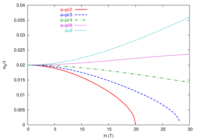
Figure 2: (Color online) Field dependence of the in-plane magnon gap for an in-plane field applied at an arbitrary angle $\phi$ with the $a$ axis, see Eq. (34). The case $\phi=0$ corresponds to the transverse-field case analyzed in Sec. IV-A, Eq. (16), while the case $\phi=\pi/2$ corresponds to a purely longitudinal field, Eq. (17), which has a spin-flop transition at $H=m_{a}$. The behavior of the gap above the spin-flop transition is described in Sec. V-A below.

V NLSM with interlayer coupling and DM interaction

Once we have established the equivalence between the semiclassical approach and the NLSM derivation of the spin-wave gaps for an ordinary easy-axis antiferromagnet, we can discuss the more general case of the model (10) where also interlayer coupling and DM interactions are present. The NLSM for this system has been already derived in Refs.MLVC, ; sces05, ; Papanicolaou, , where it has been shown that in the absence of magnetic field a 3D analogous of Eq. (23) holds:

$${\cal S}_{0}=\frac{1}{2gc}\sum_{m}\int\left\{(\partial_{\tau}{\bf n}_{m})^{2}+c^{2}(\nabla{\bf n}_{m})^{2}+\eta({\bf n}_{m}-{\bf n}_{m+1})^{2}+(D_{+}n_{m}^{a})^{2}+\Gamma_{c}(n_{m}^{c})^{2}\right\},$$ (35)

where $m$ in the layer index, ${\bf D}_{+}=D_{+}\hat{\bf x}_{a}$, $D_{+}=4Sd_{+}$, $\Gamma_{c}=32JS^{2}(\Gamma_{1}-\Gamma_{3})$ and $\eta=2JJ_{\perp}$. In this notation the in-plane and out-of-plane modes have masses:

$$m_{a}=D_{+}=4Sd_{+},\quad m_{c}=\sqrt{\Gamma_{c}}=4S\sqrt{2J(\Gamma_{1}-\Gamma_{3})},$$ (36)

in agreement with the results (19) above. Moreover, the uniform magnetization of each layer acquires an additional contribution proportional to the DM vector ${\bf D}_{+}$ with respect to Eq. (24) :

$${\bf L}_{m}=\frac{i}{8aSJ}({\bf n}_{m}\times\dot{\bf n}_{m})+\frac{1}{8aSJ}[(-1)^{m}{\bf n}_{m}\times{\bf D}_{+}+{\bf H}-{\bf n}_{m}({\bf n}_{m}\cdot{\bf H})],$$ (37)

where the oscillating factor $(-1)^{m}$ in the term proportional to ${\bf D}_{+}$ accounts for the effect of the tilting of the ochtaedra on neighboring planes, as discussed below Eq. (10). As one can easily see applying the saddle-point approach described in the previous Section to the action (35), at ${\bf H}=0$ the system orders AF below $T_{N}$ in a 3D staggered configuration, with ${\bf n}_{m}$ along $b$ in each layer. Moreover, due to the oscillating factor $(-1)^{m}$ in Eq. (37), the spins in each layer acquire a FM components ${\bf L}_{m}$, with the vectors ${\bf L}_{m}$ ordered AF in neighboring layers, see Fig. 3.

$${\bf H}=0,\quad\langle{\bf n}_{m}\rangle=\sigma_{0}\hat{\bf x}_{b},\quad\langle{\bf L}_{m}\rangle=(-1)^{m}\frac{\langle{\bf n}_{m}\rangle D_{+}}{8aSJ}=(-1)^{m}\frac{\sigma_{0}D_{+}}{8aSJ}.$$ (38)

The additional term in ${\bf D}_{+}$ in Eq. (37) translates in an additional coupling between the order parameter and ${\bf H}$ when the full NLSM action at finite magnetic field is computed:

$${\cal S}({\bf B})={\cal S}_{0}+\frac{1}{2gc}\sum_{m}\int\left[2i{\bf H}\cdot({\bf n}_{m}\times\partial_{\tau}{\bf n}_{m})-{\bf H}^{2}+({\bf H}\cdot{\bf n}_{m})^{2}-(-1)^{m}2{\bf H}\cdot({\bf n}_{m}\times{\bf D}_{+})\right].$$ (39)

As it has been discussed in Refs. MLVC, ; Thio, ; Thio90, ; Papanicolaou, ; Raman, , the effective staggered field acting on the AF order parameter due to the presence of the DM interaction makes the system an unconventional easy-axis AF. As far as the spin-waves gaps are concerned, the results of the previous Sections apply only in some specific regimes, as we shall analyze below. It is worth noting that the last three terms in Eq. (39) are proportional to:

$$-{\bf H}\cdot({\bf L}^{H}_{m}+{\bf L}^{DM}_{m}),$$ (40)

where ${\bf L}^{H}_{m}$ and ${\bf L}^{DM}_{m}$ are the contributions to ${\bf L}_{m}$ in Eq. (37) proportional to the magnetic field and to the DM term, respectively. As a consequence, the ground-state of the action (39) will be determined by the competition between the energetic cost of the bare action ${\cal S}_{0}$ and the tendency of the system to maximize the uniform spin components in the field direction, to gain energy from the term (40). Even though part of the ground-state phenomenology has been already described in Ref. Thio, ; Thio90, ; Papanicolaou, ; MLVC, ; Raman, , here we will derive these results within the general language of the saddle-point approximation for the NLSM, by focusing on the magnon-gaps behavior,Papanicolaou that will be compared with the expectation for an ordinary easy-axis AF, described in the previous Section. Then we shall also compute the effect of quantum and thermal corrections, which allows us to investigate the $(H,T_{N})$ phase diagram in the various case.

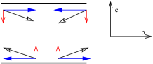
Figure 3: (Color online) Spin configuration at zero applied magnetic field in La₂CuO₄. The arrows with a solid tip represent the staggered spin components $(-1)^{m}e^{i{\bf Q}\cdot{\bf r}_{i}}{\bf n}_{i}^{m}$, the arrows with a two-lines tip represent the uniform spin components ${\bf L}_{i}^{m}$, the arrows with an open tip the full spins ${\bf S}_{i}^{m}$.

V.1 ${\bf H}$ paralell to $b$

When the field is in the $b$ direction the last term in Eq. (39) generates a staggered field along the $c$ direction which leads to a rotation of the order parameter in the $bc$ plane:Thio90 ; Papanicolaou ; Raman

$${\cal S}({\bf B})={\cal S}_{0}+\frac{1}{2gc}\sum_{m}\int\left[2iH(n_{m}^{a}\partial_{\tau}n_{m}^{c}-n_{m}^{c}\partial_{\tau}n_{m}^{a})-H^{2}[(n_{m}^{c})^{2}+(n_{m}^{a})^{2}]+2h^{m}n_{m}^{c}+i\lambda_{m}2gc({\bf n}_{m}^{2}-1)\right],$$

where we put $h^{m}=(-1)^{m}HD_{+}$ and we introduced explicitly also a set of Lagrange multipliers $\lambda_{m}$ which enforce the constraint ${\bf n}_{m}^{2}=1$ in each layer. Due to the anomalous coupling, a finite component in the $c$ direction can arise. For a generic configuration ${\bf n}_{m}=(0,\sigma^{b}_{m},\sigma^{c}_{m})$ we find the ground-state action ($m^{2}_{m}=2i\lambda_{m}gc$):

$$\bar{\cal S}_{cl}=\frac{\beta{\cal A}}{2gc}\sum_{m}\eta(\sigma_{m}^{b}-\sigma_{m+1}^{b})^{2}+\eta(\sigma_{m}^{c}-\sigma_{m+1}^{c})^{2}-2h^{m}\sigma_{m}^{c}+(m_{c}^{2}-H^{2})(\sigma_{m}^{c})^{2}+m^{2}_{m}[(\sigma_{m}^{b})^{2}+(\sigma_{m}^{c})^{2}-1].$$

The saddle-point equations then read:

$$\eta(2\sigma_{m}^{b}-\sigma_{m+1}^{b}-\sigma_{m-1}^{b})+m^{2}_{m}\sigma_{m}^{b}=0,$$

$$(m_{c}^{2}-H^{2})\sigma_{m}^{c}+h^{m}+\eta(2\sigma_{m}^{c}-\sigma_{m+1}^{c}-\sigma_{m-1}^{c})+m^{2}\sigma_{m}^{c}=0,$$

$$(\sigma_{m}^{b})^{2}+(\sigma_{m}^{c})^{2}=1.$$

At low field, one can easily check that the classical configuration is given by an order parameter with a uniform $\sigma_{b}$ component in neighboring layers and an oscillating $\sigma_{c}$ component (which corresponds to the $c$ components of the spins coming from the $(-1)^{m}e^{i{\bf Q}\cdot{\bf r}_{i}}{\bf n}^{m}_{i}$ term ordered ferromagnetically in neighboring planes, see Fig. 5):

$$\bar{\cal S}_{cl}=-\frac{\beta{\cal A}}{2gc}|\sigma_{c}|h, m^{2}_{m}=m^{2},$$

$$\sigma_{b}^{m}=\sigma_{b}=1-\sigma_{c}^{2}, \sigma_{m}^{c}=(-1)^{m}\sigma_{c}=(-1)^{m}\frac{-HD_{+}}{m_{c}^{2}+4\eta-H^{2}}.$$ (41)

In this configuration the ${\bf L}_{m}$ vectors are given by:

$${\bf L}_{m}^{H} = \frac{H}{8aSJ}\left[\sigma_{c}^{2}\hat{\bf x}_{b}-(-1)^{m}\sigma_{c}\sigma_{b}\hat{\bf x}_{c}\right],$$

$${\bf L}_{m}^{DM} = \frac{D_{+}}{8aSJ}\left[|\sigma_{c}|\hat{\bf x}_{b}+(-1)^{m}\sigma_{b}\hat{\bf x}_{c}\right],$$ (42)

so that the average (i.e. summed over neighboring layers) uniform magnetization is along $b$ and given by $\langle{\bf L}\rangle=(1/8aSJ)[D_{+}|\sigma_{c}|+H\sigma_{c}^{2}]\hat{\bf x}_{b}$. Thus, the oscillating character of $\sigma_{m}^{c}$ allows for the DM-induced magnetization to allign in the direction of the field, see Fig. 5. After inclusion of the transverse $a,c$ fluctuations, the order-parameter equations read:

$$\sigma_{b}^{2} = 1-\sigma_{c}^{2}-NI_{\perp}(m=0),$$

$$\sigma_{c} = -\frac{HD_{+}}{m_{c}^{2}+4\eta-H^{2}},\quad T<T_{N},$$ (43)

below $T_{N}$ and

$$\sigma_{b} = 0,\Rightarrow 1=\sigma_{c}^{2}+NI_{\perp}(m),$$

$$\sigma_{c} = -\frac{HD_{+}}{m_{c}^{2}+4\eta-H^{2}+m^{2}},\quad T>T_{N},$$ (44)

above $T_{N}$, where $I_{\perp}$ is computed using the matrix (32) discussed above for the case of longitudinal field. Moreover, since the system is now 3D, we have that the energy dispersion of the transverse modes is

$$\varepsilon^{2}_{a,c}({\bf k},k_{\perp})=c^{2}{\bf k}^{2}+2\eta(1-\cos k_{\perp}d)+m_{a,c}^{2},$$ (45)

where $d$ is the interlayer sapcing and an additional integration over out-of-plane momentum $k_{\perp}$ must be included in computing $I_{a,c}$. Thus, taking into account the non-diagonal character of the fluctuations matrix (32), we have for example for the $a$ mode:

$$I_{a}=\frac{1}{\beta V}\sum_{\omega_{n},{\bf k},k_{\perp}}\langle|n_{a}(\omega_{n},{\bf k},k_{\perp})|^{2}\rangle=\frac{1}{V}\sum_{{\bf k},k_{\perp}}\frac{Z_{a}({\bf k},k_{\perp})}{2\omega_{a}({\bf k},k_{\perp})}\coth\frac{\beta\omega_{a}({\bf k},k_{\perp})}{2}+\frac{Z_{c}({\bf k},k_{\perp})}{2\omega_{c}({\bf k},k_{\perp})}\coth\frac{\beta\omega_{c}({\bf k},k_{\perp})}{2},$$ (46)

where $V$ is the 3D volume of the system. Here $\omega_{a,c}$ are the generalization of Eq. (17) at finite momentum:

$$\omega^{2}_{a,c}({\bf k},k_{\perp})=\frac{\varepsilon_{c}^{2}+\varepsilon_{a}^{2}}{2}+H^{2}\pm\sqrt{\left(\frac{\varepsilon_{c}^{2}-\varepsilon_{a}^{2}}{2}\right)^{2}+4H^{2}\left(\frac{\varepsilon_{c}^{2}+\varepsilon_{a}^{2}}{2}\right)},$$ (47)

where the explicit dependence of $\varepsilon_{a,c}$ on momenta has been omitted. Analogously, the spectral weights $Z_{a,c}$ of the two poles are given by:

$$Z_{a,c}({\bf k},k_{\perp})=\pm\frac{-\omega_{a,c}^{2}+\varepsilon_{c}^{2}({\bf k},k_{\perp})-H^{2}}{\omega_{c}^{2}({\bf k},k_{\perp})-\omega_{a}^{2}({\bf k},k_{\perp})},$$ (48)

and are plotted in the inset of Fig. 4 for $k_{\perp}=0$ as a function of $ka$. Note that since in all the formulas the magnetic field is measured in units of $g_{s}\mu_{B}\approx 0.1$ meV, and since typical values of $J$ are of the order of 130 meV, we used for simplicity the equivalence $H=1$ T=$10^{-3}J$.

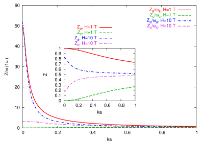
Figure 4: (Color online) Momentum dependence of the spectral weight corresponding to the poles at $\omega_{a}({\bf k},k_{\perp})$ or $\omega_{c}({\bf k},k_{\perp})$ in Eq. (46). Here $k_{\perp}=0$, $m_{a}=0.02J,m_{c}=0.05J,c=J$, and we used units such that H=1 T corresponds to $10^{-3}J$. Inset: momentum dependence of $Z_{a},Z_{c}$ defined in Eq. (48). Observe that even thought $Z_{a}\approx Z_{c}$ at $H=10$ T as $ka\sim 0.5$ the contribution at $k=0$ is always predominant in the momentum sum (46), due to the fact that the $a$ gap softens as the field strenght increases.

Due to the thermal factors, the main contribution in the momentum integration in Eq. (46) comes from ${\bf k}=k_{\perp}=0$, where also the factors $Z_{\alpha}/\omega_{a}$ have the largest value, see Fig. 4. As a consequence, we can safely approximate the momentum dependence of Eq. (47) with

$$\omega^{2}_{a,c}({\bf k},k_{\perp})\approx\omega^{2}_{a,c}+c^{2}{\bf k}^{2}+2\eta(1-\cos k_{\perp}d),$$ (49)

where $\omega_{a,c}$ are the magnon gaps given in Eq. (17), and we can neglect the momentum dependence of $Z_{a,c}$ in Eq. (46). We thus obtain below $T_{N}$:

$$I_{a}=Z_{a}(0)I_{3D}(\omega_{a})+Z_{c}(0)I_{3D}(\omega_{c}),$$ (50)

where $I_{3D}(M)$ is the extension to the layered 3D case of the integral (30):

$$I_{3D}(M)=\frac{gT}{2\pi c}\int_{-\pi}^{\pi}\frac{dz}{2\pi}\ln\left\{\frac{\sinh(c\Lambda/2T)}{\sinh\sqrt{M^{2}+2\eta(1-\cos z)}/2T}\right\}.$$ (51)

Above $T_{N}$ we simply substitute $\omega_{a,c}^{2}\rightarrow\omega_{a,c}^{2}+m^{2}$ in Eq. (50), where as usual $m^{2}$ plays the role of the inverse correlation length, to be obtained solving the self-consistency equation (44). As far as the $c$ fluctuations are concerned, the previous result is clearly reversed, with a larger contribution coming from the pole at $\omega_{c}$, since now $Z_{a,c}(0)=\mp(-\omega_{a,c}^{2}+m_{a}^{2}-H^{2})/(\omega_{c}^{2}-\omega_{a}^{2})$.

As the field strength increases we see that, according to Eq. (17), the smaller gap $\omega_{a}$ decreases, and vanishes at the critical field:

$$H_{c}^{(1)}=m_{a}=D_{+}.$$ (52)

Indeed, at $H_{c}^{(1)}$ we have a spin-flop transition: the in-plane component of the order parameter rotate from the $b$ to the $a$ direction, so that the classical configuration becomes:

$${\bf n}_{m}=(\sigma_{a},0,(-1)^{m}\sigma_{c}).$$ (53)

The uniform magnetization changes correspondingly:

$${\bf L}_{m}^{H}=\frac{H}{8aSJ}\hat{\bf x}_{b},\quad{\bf L}_{m}^{DM}=\frac{D_{+}}{8aSJ}|\sigma_{c}|\hat{\bf x}_{b},$$ (54)

and jumps discontinously at the spin-flop transition by a quantity $H[1-\sigma_{c}(H_{c}^{(1)})]/8aSJ$, see Fig. 5.

Figure 5: (Color online) Magnetic-field dependence at of the spins ground state and of the $T=0$ average uniform magnetization in the field direction for a field along the $b$ axis. At finite magnetic field the order-parameter ${\bf n}$ rotates in the $bc$ plane. The spin configuration is determined as usual by ${\bf S}_{i}/S=(-1)^{m}e^{i{\bf Q}\cdot{\bf r}_{i}}{\bf n}_{i}^{m}+{\bf L}_{i}^{m}$, where the staggered and uniform components are indicated by arrows with different tips as in Fig. 3: the arrows with a two-lines tip represent the uniform components ${\bf L}_{m}$ and the arrows with a solid tip the staggered components $(-1)^{m}e^{i{\bf Q}\cdot{\bf r}_{i}}{\bf n}_{i}^{m}$. At $H<H_{c}^{(1)}\approx 18$ T (left in the figure) ${\bf n}_{m}$ is defined in Eq. (41) and ${\bf L}_{m}$ in Eq. (42), so that the spins have both the staggered and uniform component in the $bc$ plane. The uniform components are due both to the magnetic field and to the DM interaction, see Eq. (42), and the sum of ${\bf L}_{M}+{\bf L}_{m+1}$ is alligned along the field. Above the spin-flop transition (right in the figure) the staggered components ${\bf n}_{m}$ lie in the $ac$ plane see Eq. (53) (so that the part along $a$ is orthogonal to the plane of the figure and indicated by a cross) and the uniform components ${\bf L}_{m}$ point along $b$, see Eq. (54). The order-parameter values used to evaluate the $\langle{\bf L}\rangle$ are the same reported in Fig. 7. Observe that since in our approximation the critical field $H_{c}^{(1)}$ is independent of temperature, as well as $\sigma_{c}$, the uniform magnetization is temperature independent below $T_{N}$.

By adding $b$ and $c$ fluctuations around this ground-state solution we obtain the new saddle-point equations:

$$\sigma_{a}^{2} = 1-\sigma_{c}^{2}-N\tilde{I}_{\perp}(m=0),$$

$$\sigma_{c} = -\frac{HD_{+}}{m_{c}^{2}+4\eta-m_{a}^{2}},\quad T<T_{N},$$ (55)

and

$$\sigma_{a} = 0,\Rightarrow 1=\sigma_{c}^{2}+N\tilde{I}_{\perp}(m),$$

$$\sigma_{c} = -\frac{HD_{+}}{m_{c}^{2}+4\eta-m_{a}^{2}+m^{2}},\quad T>T_{N},$$ (56)

where $\tilde{I}_{\perp}$ accounts for the $b,c$ fluctuations described by the inverse matrix:

$$\hat{G}^{-1}=\left(\begin{array}[]{cc}\omega^{2}({\bf q})+H^{2}-m_{a}^{2}+m^{2}&0\\ 0&\omega^{2}({\bf q})+m_{c}^{2}-m_{a}^{2}+m^{2}\end{array}\right),$$ (57)

where $\omega^{2}({\bf q})=\omega_{n}^{2}+c^{2}{\bf k}^{2}+2\eta(1-\cos k_{\perp}d)$. As far as the magnon gaps are concerned, we see that above the transition the field in the $b$ direction acts as a transverse field, since the direction of the magnetization has changed. Once again, the behavior of the magnon gaps can be easily read from the Green’s function matrix (57). We find that the in-plane mode corresponds now to a fluctuation of the $b$ component, with a field-dependent mass, while the out-of-plane mode does not depend on the field but should be rescaled with respect to the $m_{a}$ gap:

$$\omega^{2}_{in}\equiv\omega_{b}^{2}=\sqrt{H^{2}-m_{a}^{2}},\quad\omega_{c}^{2}=\sqrt{m_{c}^{2}-m_{a}^{2}}.$$ (58)

The resulting field dependence of the magnon gaps is reported in Fig. 6.

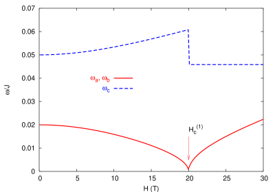
Figure 6: (Color online) Field dependence of the magnon gaps at $T=0$ for a field applied along the $b$ axis. We used $m_{a}=0.02J,m_{c}=0.05J$, and units such that H=1 T corresponds to $10^{-3}J$, so that the first critical field $H_{c}^{(1)}=D_{+}=m_{a}=20$ T. Below $H_{c}^{(1)}$ the in-plane and out-of-plane mode are correspond to $a$ and $c$ component fluctuations, whose gaps are given by $\omega_{a}$ and $\omega_{c}$ in Eq. (17), respectively. Above the critical field the in-plane mode corresponds to fluctuations of the $b$ component, and the magnon gaps are defined by Eq. (58).

By further increasing $H$ one will finally reaches a second critical field above which the transverse in-plane component of the staggered order parameter vanishes, $\sigma_{a}=0$, but the $\sigma_{c}$ component is still nonzero, see Fig. 7. Since by definition $|{\bf n}|<1$, we can see from Eq. (55) that the solution (53) is valid only when $\sigma_{c}\leq 1$, so at fields lower than Thio90 ; Papanicolaou :

$$H_{c}^{(2,naive)}=(m^{2}_{c}+4\eta-m_{a}^{2})/D_{+}.$$ (59)

However, the estimate (59) does not take into account quantum fluctuations, which reduce the $T=0$ value of the in-plane order parameter according to Eq. (43). Since the transverse fluctuations $I_{\perp}$ do not depend strongly on the magnetic field, one can see that the second critical field, defined as the field at which $\sigma_{a}(T=0)=0$ in Eq. (55), is given approximately by:

$$H_{c}^{(2)}\simeq\frac{m^{2}_{c}+4\eta-m_{a}^{2}}{D_{+}}\sigma_{0}(H=0,T=0),$$ (60)

where $\sigma_{0}(H=0)=\sqrt{1-NI_{\perp}(T=0,H=0)}$ is the magnetization of the system measured at $T=0$ along the $b$ axis without external magnetic field. Observe that quantum corrections can indeed reduce considerably the second critical field.

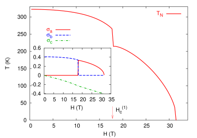
Figure 7: (Color online) Phase diagram of the system for ${\bf H}\parallel b$. The parameter values are chosen to reproduce the data of La₂CuO₄, i.e. $D_{+}=m_{a}=0.0116J$, $m_{c}=0.034J$, $J=130$ meV, $\rho_{s}=0.07J$ and $c=1.3J$ MLVC . For the interlayer coupling we used $\eta=8\times 10^{-5}J^{2}$, which correctly reproduce the spin-flop transition measured in Ref. Gozar, for ${\bf H}\parallel c$, see end of Sec. V-B. The magnetic field is converted in energy trough $H\rightarrow g_{s}\mu_{B}H$, where $\mu_{B}$ is the Bohr magneton and $g_{s}=2.1$ is the gyromagnetic ratio in the $b$ direction. Inset: field evolution of the staggered order parameter components at $T=0$ in the various phases.

In Fig. 7 we report as an example the phase diagram for La₂CuO₄ of the transition temperature $T_{N}$ vs $H$ obtained in the saddle-point approximation. By estimating the parameter values from the Raman measurements of the magnon gaps in Ref. Gozar, (see also theo-exp, ), we choose $m_{a}=0.0116J$, $m_{c}=0.034J$, $\eta=8\times 10^{-5}J^{2}$, with $J=130$ meV and $g_{s}=2.1$, as appropriate for the $b$ direction. For the stiffness and spin-wave velocity we use $\rho_{s}=0.07J$ and $c=1.3J$ respectively, which are not far from the standard values quoted in the literature CHN ; CSY and have been shown to be appropriate to reproduce (in the same approximation) the uniform-susceptibility data MLVC . In the inset we also report the $T=0$ value of the order-parameter components as a function of the field. As we can see, below $H_{c}^{(1)}=D_{+}$, $\sigma_{a}=0$ and $\sigma_{b}\neq 0$, while the situation is reversed above the spin-flop transition. The component $\sigma_{c}$ is continuous at the spin-flop transition. In principle, its slope as a function of the magnetic field changes at the spin-flop transition according to Eqs. (43) and (55). However, for the parameter values used here, as appropriate for La₂CuO₄, this change is almost undistinguishable in Fig. 7. Moreover, also the magnitude of the in-plane component is continuous at the transition, the change being only in its direction.

As far as the second critical field is concerned, it turns out that Eq. (60), which uses the value of $\sigma_{0}$ at $H=0$, is an excellent estimate of the second critical field $H_{c}^{(2)}$, obtained by means of the self-consistent value $1-N\tilde{I}_{\perp}(H)$: indeed, since we found $\sigma_{0}(T=0,H=0)=0.4$ (see inset), and $H_{c}^{(2,naive)}=77$ T, Eq. (60) would give $H_{c}^{(2)}=30.8$ T, which is almost the value found numerically, see Fig. 7. It is worth noting that $H_{c}^{(2)}$ has been measured recently in $1\%$ doped La_2-xSr_xCuO₄ sample by Ono et al. Ono , who found $H_{c}^{(2)}\simeq 20$ T. Thus, even though $H_{c}^{(2)}$ has not been measured in undoped La₂CuO₄, where it is expected to be larger than in the $1\%$ doped sample, the value of 30 T following from Eq. (60) seems more realistic than the bare estimate (59), which gives 77 T. Observe that neglecting the quantum renormalization of the order parameter in the estimate of the second critical field can lead to an underestimate of the mass of the $c$ mode, as it has been done in Ref. Thio90, , where Eq. (59) has been used.

Fibally, we note that in the saddle-point approximation used so far the transverse gaps are constant in temperature below $T_{N}$. However, one would expect that a better approximation could reproduce the softening of the transverse gaps as the temperature increases, as observed experimentally. In this case also the value of the first critical field $H_{c}^{(1)}$ would acquire a temperature dependence, which is instead absent in the phase diagram of Fig. 7. Moreover, this could also smoothen the discontinuity of $T_{N}$ at the spin-flop transition found at saddle-point level.

V.2 ${\bf H}$ parallel to $c$

When ${\bf H}$ is along the $\hat{\bf x}_{c}$ direction the last term in the action (39) gives rise to an effective longitudinal staggered field:

$${\cal S}({\bf B})={\cal S}_{0}+\frac{1}{2gc}\sum_{m}\int\left[2iH(n_{m}^{b}\partial_{\tau}n_{m}^{a}-n_{m}^{a}\partial_{\tau}n_{m}^{b})-H^{2}+H^{2}(n_{m}^{c})^{2}]+2h^{m}n_{m}^{b}+i\lambda_{m}2gc({\bf n}_{m}^{2}-1)\right].$$ (61)

Following the line of the analysis performed in the previous section, we first determine the ground-state configuration in the presence of the magnetic field. Since also the effective staggered field is longitudinal, we do not expect in this case to have a change of direction of the equilibrium configuration. We can then look for a ground-state solution of the form ${\bf n}_{m}=\sigma_{m}^{0}\hat{\bf x}_{b}$, which gives:

$$\bar{\cal S}_{cl}=\frac{\beta{\cal A}}{2gc}\sum_{m}\eta(\sigma_{m}^{0}-\sigma_{m+1}^{0})^{2}+2h^{m}\sigma_{m}^{0}+m^{2}_{m}[(\sigma_{m}^{0})^{2}-1].$$ (62)

The saddle-point equations then read

$$\eta(2\sigma_{m}^{0}-\sigma_{m+1}^{0}-\sigma_{m-1}^{0})+h^{m}+m^{2}_{m}\sigma_{m}^{0}=0,$$

$$(\sigma_{m}^{0})^{2}=1.$$ (63)

As a consequence, two solutions are possible: (i) the order parameter is the same in all the layers, and the ground-state action $\bar{\cal S}_{cl}$ vanishes:

$$\sigma_{m}^{0}=\sigma_{0}=-1,\quad m^{2}=-(-1)^{m}h/\sigma_{0}=(-1)^{m}h,\quad\bar{\cal S}_{cl}=0.$$ (64)

This configuration is the same of the case without magnetic field. The uniform spin components are:

$${\bf L}_{m}^{H}=\frac{H}{8aSJ}\hat{\bf x}_{c},\quad{\bf L}_{m}^{DM}=(-1)^{m}\frac{D_{+}}{8aSJ}|\sigma_{0}|\hat{\bf x}_{c},$$ (65)

so that the ${\bf L}_{m}^{DM}$, which are ordered antiferromagnetically in neighboring layers (see Fig. 3), do not contribute to the average uniform magnetization $\langle{\bf L}\rangle={\bf L}^{H}$ (see Fig. 8), but one takes advantage from the out-of-plane antiferromagnetic coupling; (ii) the order parameter change sign in neighboring layers, which means that the spins order ferromagnetically in the $c$ direction, with the moment ${\bf L}_{m}^{DM}$ oriented in the same direction:

$${\bf L}_{m}^{H}=\frac{H}{8aSJ}\hat{\bf x}_{c},\quad{\bf L}_{m}^{DM}=\frac{D_{+}}{8aSJ}|\sigma_{0}|\hat{\bf x}_{c},$$ (66)

giving $\langle{\bf L}\rangle=(H+D_{+}|\sigma_{0}|)/8aSJ$. This spin flop of the uniform $c$ components of the spins leads to a lowering of the energy when the gain in magnetic energy is larger than the cost coming from the interlayer AF coupling. Observe that the average uniform magnetization jumps discontinuosly at the spin-flop transition, the jump being proportional to $\sigma_{0}$, so that it decreases as the temperature increases, see Fig. 8.

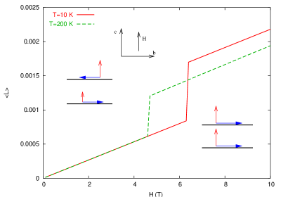
Figure 8: (Color online) Magnetic-field dependence of the spin configuration and of the average uniform magnetization at two different temperatures for a field along the $c$ axis. The spin configuration is determined as usual by ${\bf S}_{i}/S=(-1)^{m}e^{i{\bf Q}\cdot{\bf r}_{i}}{\bf n}^{m}+{\bf L}^{m}$, where the staggered and uniform components are indicated by arrows with different tips as in Fig. 3 and Fig. 5. At $H<H_{c}$, where $H_{c}=6$ T at $T=10$ K and $H_{c}=4.6$ at $T=200$ K, see also Fig. 10 below, the system has 3D antiferromagnetic order as described by Eq. (64). The difference between the ${\bf L}_{m}$ components (arrows with a two-lines tip) in neighboring planes is due to the DM-induced term ${\bf L}_{m}^{DM}$ which changes sign from one layer to the next one, while ${\bf L}_{m}^{H}$ is always parallel to ${\bf H}$, see Eq. (65). Above the spin flop the spins are ordered ferromagnetically in neighboring layers, see Eq. (67), allowing for the uniform ${\bf L}_{m}$ components to allign along the field in all the layers. The jump at the transition is proportional to the order parameter $\sigma_{0}$, and decreases as the temperature increases, see inset of Fig. 10.

The classical action in this configuration is:

$$\sigma_{m}^{0}=(-1)^{m}\sigma_{0}=-1,\quad m^{2}_{m}=m^{2}=-h/\sigma_{0}-4\eta=h-4\eta,\quad\bar{\cal S}_{cl}=\frac{\beta{\cal A}N_{l}}{gc}\left(-h+2\eta\right),$$ (67)

where $N_{l}$ is the number of layers. When $h>2\eta$ this second solution becomes energetically favorable, so that the critical field for this spin-flop transition is:

$$H_{c}=\frac{2\eta}{D_{+}}.$$ (68)

When transverse fluctuations are included the first of Eqs. (63) will not change, while the value of the order parameter $\sigma_{0}$ will acquire quantum and thermal corrections due to transverse fluctuations, according to:

$$\sigma_{0}^{2}=1-I_{\perp}(h/\sigma_{0}).$$ (69)

In Eq. (69) we included the explicit dependence of the transverse fluctuations on the order parameter $\sigma_{0}$ via the effective staggered field $h$, as we will derive in detail below. To determine $I_{\perp}$ we should distinguish the case below and above the spin-flop transition. Let us first consider the case (64) of low field. Since the Lagrange multiplier is oscillating in neighboring layers, it gives rise to a coupling between the transverse modes at $k_{\perp}$ and $k_{\perp}+Q_{\perp}$, where $Q_{\perp}=\pi/d$. We then have:

$${\cal S}=\bar{\cal S}_{cl}+\frac{1}{2}\sum_{\alpha=a,c}\sum^{\prime}_{{\bf k},k_{\perp}}\Psi^{+}_{\alpha}({\bf k},k_{\perp})\hat{G}_{\alpha}^{-1}\Psi_{\alpha}({\bf k},k_{\perp}),$$

where $\Psi^{+}_{\alpha}({\bf k},k_{\perp})=((n_{\alpha}({\bf k},k_{\perp}),n_{\alpha}({\bf k},k_{\perp}+Q_{\perp}))$, the sum $\sum^{{}^{\prime}}_{k_{\perp}}$ is over the reduced Brilluoin zone for $k_{\perp}$, i.e $0\leq k_{\perp}\leq\pi/d$. The Green’s function for each mode is now a matrix. For the $a$ mode we find:

$$\hat{G}_{a}^{-1}=\frac{1}{gc}\left(\begin{array}[]{cc}\omega_{n}^{2}+\omega^{2}({\bf k},k_{\perp})&m^{2}\\ m^{2}&\omega_{n}^{2}+\omega^{2}({\bf k},k_{\perp}+Q_{\perp})\end{array}\right),$$ (70)

with $\omega^{2}({\bf k},k_{\perp})=m_{a}^{2}+c^{2}{\bf k}^{2}+2\eta(1-\cos k_{\perp}d)$ and $m^{2}=-h/\sigma_{0}$, according to Eq. (64). The inverse Green’s function for the $c$ mode has an analogous expression, except that $m_{a}^{2}\rightarrow m_{c}^{2}+H^{2}$. After integration of the Gaussian fluctuations one obtains the order-parameter equation (69), provided that Eq. (70) is used to compute the fluctuations:

$$\langle|n_{a}(\omega_{n},{\bf k},k_{\perp})|^{2}\rangle=\frac{\omega_{n}^{2}+\omega^{2}({\bf k},k_{\perp}+Q_{\perp})}{{\rm det}\,\hat{G}_{a}}.$$ (71)

The integral of the $a$-mode fluctuations has a structure similar to the one of Eq. (46), with two contributions at the eigenvalues of the matrix $\hat{G}_{a}$:

$$I_{a}=\frac{1}{\beta V}\sum_{\omega_{n},{\bf k},k_{\perp}}\langle|n_{a}(\omega_{n},{\bf k},k_{\perp})|^{2}\rangle=\frac{1}{V}\sum_{{\bf k},k_{\perp}}\frac{Z_{+}(k_{\perp})}{2\omega_{+}({\bf k},k_{\perp})}\coth\frac{\beta\omega_{+}({\bf k},k_{\perp})}{2}+\frac{Z_{-}(k_{\perp})}{2\omega_{-}({\bf k},k_{\perp})}\coth\frac{\beta\omega_{-}({\bf k},k_{\perp})}{2},$$ (72)

where

$$\omega^{2}_{\pm}({\bf k},k_{\perp}) = \frac{\varepsilon_{a}^{2}({\bf k},k_{\perp})+\varepsilon_{a}^{2}({\bf k},k_{\perp}+Q_{\perp})}{2}\pm\sqrt{\left(\frac{\varepsilon_{a}^{2}({\bf k},k_{\perp})-\varepsilon_{a}^{2}({\bf k},k_{\perp}+Q_{\perp})}{2}\right)^{2}+m^{2}}=$$ (73)

$$= c^{2}{\bf k}^{2}+m_{a}^{2}+2\eta\pm\sqrt{4\eta^{2}\cos^{2}k_{\perp}d+m^{2}}.$$

Analogously to the case discussed in the previous section, the spectral weights $Z_{\pm}$ of the two poles are not equivalent, and determine the main character of the excitation. In this case we have:

$$Z_{\pm}(k_{\perp})=\mp\frac{-\omega_{\pm}^{2}+\omega^{2}({\bf k},k_{\perp}+Q_{\perp})}{\omega_{+}^{2}({\bf k},k_{\perp})-\omega_{-}^{2}({\bf k},k_{\perp})}=\mp\frac{2\eta\cos k_{\perp}d\mp\sqrt{4\eta^{2}\cos^{2}k_{\perp}d+m^{2}}}{2\sqrt{4\eta^{2}\cos^{2}k_{\perp}d+m^{2}}}.$$ (74)

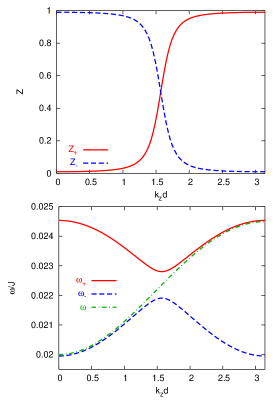
Figure 9: (Color online) Low panel: out-of-plane momentum $k_{z}\equiv k_{\perp}$ dependence of the two solutions $\omega_{\pm}$ of Eq. (73) at ${\bf k}=0$, compared to the momentum dependence of the function $\omega({\bf k}=0,k_{\perp})=\sqrt{m_{a}^{2}+2\eta(1-\cos k_{\perp}d)}$. We used $D_{+}=m_{a}=0.02J$ and $H=1$ T$=10^{-3}$ J. Observe the small difference of $\omega_{-}$ with respect to $\omega$ at $k_{\perp}=0$. Top panel: momentum dependence of the spectral weight $Z_{\pm}(k_{\perp})$ defined in Eq. (74). As one can see, at small momentum $Z_{-}\gg Z_{+}$, while at $k_{\perp}d>\pi/2$ the situation is reversed. As a consequence, the momentum sum in Eq. (72) select always between $\omega_{+}$ and $\omega_{-}$ the solution which follows most closely the momentum dependence of the solution $\omega(k_{\perp})$ of the case $H=0$.

The momentum dependence of $Z_{\pm}$ is reported in the top panel of Fig. 9, while in the lower panel the two solutions $\omega_{\pm}({\bf k}=0,k_{\perp})$ are plotted. As one can see, as $k_{\perp}$ increases the spectral weigh of the momentum sum in Eq. (72) moves from the solution $\omega_{-}(k_{\perp})$ to the solution $\omega_{+}(k_{\perp})$, which follow closely the bare function $\omega(k_{\perp})$ in the two regimes $0<k_{\perp}d<\pi/2$ and $\pi/2<k_{\perp}d<\pi$ respectively. The effect of the magnetic field is then twofold: it affects the magnon gap $k_{\perp}=0$ and opens an additional one at $k_{\perp}d=\pi/2$. To compute explicitly the momentum sum in Eq. (72) we can observe that $Z_{\pm}(k_{\perp})$ only depend on the out-of-plane momentum $k_{\perp}$. We can then perform the usual integration over the in-plane momentum ${\bf k}$ in Eq. (72), obtaining an expression similar to Eq. (50)-(51):

$$I_{a}=\frac{gT}{2\pi c}\int_{-\pi}^{\pi}\frac{dz}{2\pi}Z_{-}(z)\ln\left\{\frac{\sinh(c\Lambda/2T)}{\sinh A_{-}(z)/2T}\right\}+Z_{+}(z)\ln\left\{\frac{\sinh(c\Lambda/2T)}{\sinh A_{+}(z)/2T}\right\},\quad H<H_{c}$$ (75)

where

$$A_{\pm}(z)=\sqrt{m_{a}^{2}+2\eta\pm\sqrt{4\eta^{2}\cos z+(HD_{+}/\sigma_{0})^{2}}}.$$ (76)

For the $c$ fluctuations one finds the same results, provided that $m_{a}^{2}\rightarrow m_{c}^{2}+H^{2}$ in all the above formulas.

Let us discuss now the issue of the magnon gaps. The spectral function of the $a$ mode at ${\bf k}=0,k_{\perp}=0$ has a two-poles structure analogous to Eq. (33), i.e.:

$${\cal A}_{a,c}(\omega>0)=\left[\frac{Z_{+}(k_{\perp}=0)}{\omega_{+}}\delta(\omega-\omega_{+})+\frac{Z_{-}(k_{\perp}=0)}{\omega_{-}}\delta(\omega-\omega_{-})\right].$$

However, as observed before and shown in Fig. 9, at $k_{\perp}=0$ is $Z_{-}/\omega_{-}\gg Z_{+}/\omega_{+}$, so that only the second term contributes in the previous equation and allows us to identify the magnon gap as the ${\bf k}=0,k_{\perp}=0$ limit of the the function $\omega_{-}({\bf k},k_{\perp})$ above, i.e.:

$$\omega^{2}_{a} = m_{a}^{2}+2\eta-\sqrt{4\eta^{2}+\left(\frac{HD_{+}}{\sigma_{0}}\right)^{2}},$$

$$\omega^{2}_{c} = m_{c}^{2}+H^{2}+2\eta-\sqrt{4\eta^{2}+\left(\frac{HD_{+}}{\sigma_{0}}\right)^{2}},\quad H<H_{c},$$ (77)

which reduce to the conventional ones when $H=0$. Here we used explicitly that $m^{2}=-h/\sigma_{0}$, according to Eq. (64). Observe that this result is quite different from the interpretation given in Ref. Papanicolaou, , where it was claimed that the acoustic and optical modes are mixed. Instead, at $k_{\perp}=0$ only the mode $\omega_{-}$ is observed, as Raman measurements confirm.Gozar ; theo-exp Moreover, we stress that according to the discussion below Eq. (16), for an ordinary easy-axis AF we expected that $\omega_{a}$ is unchanged and $\omega_{c}$ hardens for a field parallel to $c$. Instead, due to the presence of the DM interaction, the two modes have a field dependence $\sim-H^{2}\gamma_{a,c}$, with $\gamma_{a}=D_{+}^{2}/(4\eta\sigma_{0}^{2})$ and $\gamma_{c}=-1+D_{+}^{2}/(4\eta\sigma_{0}^{2})$. As a consequence, the $a$ mode always softens, while the behavior of the $c$ mode depends on the ratio $D_{+}^{2}/(4\eta\sigma_{0})$.

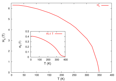
Figure 10: (Color online) $H_{c}-T$ phase diagram for ${\bf H}\parallel c$. We used the same parameter values as Fig. 7, except that in this case $g_{s}=2.4$, as appropriate for a field in the $c$ direction theo-exp . The order parameter $\sigma_{0}(T)$ has been determined self-consistently trough Eq. (69), computing the transverse fluctuations with Eq. (75) and (80) below and above the spin-flop transition, respectively, where the critical field $H_{c}$ is defined trough Eq. (81). Inset: temperature dependence of the staggered order parameter at $H=1$ T.

Let us analyze now the case $H>H_{c}$. According to Eq. (67) we find a uniform saddle-point value of the constraint, $m^{2}_{m}=m^{2}=-h/\sigma_{0}-4\eta$, so that the matrix of the transverse fluctuations is again diagonal in momentum space:

$$\hat{G}^{-1}=\left(\begin{array}[]{cc}\omega_{n}^{2}+c^{2}{\bf k}^{2}-2\eta(1+\cos k_{\perp}d)+m_{a}^{2}-h/\sigma_{0}&0\\ 0&\omega_{n}^{2}+c^{2}{\bf k}^{2}-2\eta(1+\cos k_{\perp}d)+m_{c}^{2}+H^{2}-h/\sigma_{0}\end{array}\right).$$ (78)

However, in the classical configuration (67) the spins are order ferromagnetically in neighboring planes, see Fig. 8: this means that the low-energy spin fluctuations are those at $k_{\perp}=\pi/d$ in the notation of Eq. (78), so that the spin-wave gaps evolve at $H>H_{c}$ in:

$$\omega^{2}_{a} = m_{a}^{2}+\left(\frac{HD_{+}}{|\sigma_{0}|}\right),$$

$$\omega^{2}_{c} = m_{c}^{2}+H^{2}+\left(\frac{HD_{+}}{|\sigma_{0}|}\right),\quad H>H_{c}.$$ (79)

Since the matrix (78) admits two simple poles, the transverse fluctuations are described by the function (51), whith the masses given by the previous equation:

$$I_{a,c}=I_{3D}(\omega_{a,c}),\quad H>H_{c}$$ (80)

Observe that both for the case $H<H_{c}$ and $H>H_{c}$ the integral of transverse fluctuations, given by Eqs. (75) and (80) respectively, depend explicitly on the Lagrange multiplier $h/\sigma_{0}$, so that Eq. (69) is a self-consistency equation for the order parameter at all the temperatures. This is quite different with respect to all the cases analyzed before, where $I_{\perp}$ depends only on the transverse masses and two separate regimes exist, $m^{2}=0,\sigma_{0}\neq 0$ below $T_{N}$, and $m^{2}\neq 0$ and $\sigma_{0}=0$ above $T_{N}$ (see Eq. (28)). Here instead, due to the effective longitudinal field $h^{m}$ in Eq. (61), instead of the two regimes we obtain a single self-consistent equation (69) valid at all the temperatures. As a consequence, exactly as for a ferromagnet in the presence of the external field, the order parameter never vanishes, and the transition transforms into a crossover from a regime where $\sigma_{0}$ is large to one where $\sigma_{0}$ is small MLVC . This is shown in the inset of Fig. 10, where we obtained $\sigma_{0}(T)$ at $H=1$ T by solving numerically the self-consistency equation (69) at various temperature. It is worth noting that once that transverse fluctuations are included, also the definition of the critical field (68) changes. Indeed, since in general $\sigma_{0}$ is lower than 1 (including $T=0$ due to quantum correction), the critical field becomes itself a function of temperature. A first estimate of this effect can be done by evaluating again the value of the action $\bar{\cal S}_{cl}$ in Eq. (67) for a generic $\sigma_{0}$. We then obtain that the critical field is:

$$H_{c}=\frac{4\eta}{D_{+}}\frac{\sigma_{0}}{(1+\sigma_{0}^{2})}.$$ (81)

A more precise evaluation of $H_{c}$ could be done including also the contribution of the Gaussian transverse fluctuations to the action (70). However, already Eq. (81) allows one to recognize that as the temperature increases the decrease of the order parameter $\sigma_{0}$ induces also a decrease of the critical field for the spin-flop transition. The resulting $H_{c}-T$ phase diagram, obtained by means of Eq. (81) where $\sigma_{0}$ is the solution of the self-consistent Eq. (69), is reported in Fig. 10.

Once that we determined self-consistently the values of the order parameter and of the critical field, we can also compute the field dependence of the magnon gaps. In Fig. (11) we show the field dependence at $T=0$ of $\omega_{a}$ and $\omega_{c}$, as given by Eqs. (77) and (79) below and above the spin-flop transition, respectively. For the interlayer coupling $\eta$ we used the value $\eta=8\times 10^{-5}J^{2}$, which allows us to obtain a critical field at low temperature around 6.5 T, as the one measured experimentally Gozar . Observe that this value of $\eta$ is quite similar to the one obtained in Ref. theo-exp, from the jump of the experimental measured in-plane gap at $H_{c}$, even though such an estimate is done neglecting quantum corrections to the order parameter. With this parameter values we find that the below the spin-flop transition also the $c$ mode is slightly decreasing.

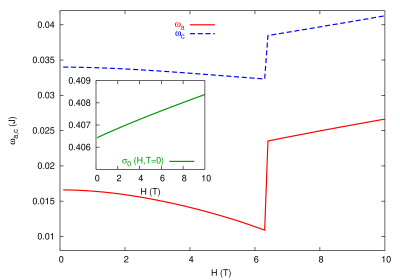
Figure 11: (Color online) Field dependence of the magnon gaps at $T=0$ for $H\parallel c$. Here $H_{c}\approx 6.5$T, so below it the gap decrease according to Eq. (77), while above it they increase according to Eq. (79). The parameter values are the same of Fig. (10). Inset: field dependence of the zero-temperature order parameter.

V.3 ${\bf H}$ parallel to $a$

Finally, let us consider the case of a field along $\hat{\bf x}_{a}$, i.e. parallel to the direction of the DM vector ${\bf D}_{+}$. In this case, the last term of Eq. (39) vanishes, and the system behaves as a conventional easy-axis AF. As a consequence, Eq. (16) holds, giving a hardening of the $a$ gap and leaving the $c$ gap unchanged.

VI Conclusions

We have investigated the field dependence of the magnetic spectrum in anisotropic two-dimensional and Dzyaloshinskii-Moriya layered antiferromagnets. Starting from the appropriate spin-Hamiltonian for each case, we obtained the magnon gaps and spectral intensities as a function of the applied magnetic field, and we discussed the various possible ground state configurations and phase diagram. In particular, we showed that the peculiar coupling of the magnetic field with the staggered order parameter induced by the DM interaction gives rise to very interesting magnetic phenomena, such as spin-flop transitions and rotation of spin quantization basis. The predictions of the theory developed in this article are now ready to be compared with Raman spectroscopy experiments in Sr₂CuO₂Cl₂ and La₂CuO₄, reported in the forthcoming article.theo-exp

VII Acknowledgements

The authors would like to acknowledge invaluable discussions with A. Lavrov.

References

- (1) I. E. Dzyaloshinskii, J. Phys. Chem. Solids 4, 241 (1958).
- (2) T. Moriya, Phys. Rev. Lett. 4, 228 (1960).
- (3) D. Talbayev, L. Mihály and J. Zhou, Phys. Rev. Lett. 93, 017202 (2004).
- (4) M. D. Lumsden, B. C. Sales, D. Mandrus, S. E. Nagler, and J. R. Thompson, Phys. Rev. Lett. 86, 159 (2001).
- (5) V. N. Kotov, M. E. Zhitomirsky, M. Elhajal and F. Mila, Phys. Rev. B70, 214401 (2004).
- (6) A. L. Chernyshev, Phys. Rev. B72, 174414 (2005).
- (7) L. Shekhtman, O. E. Wohlman, and A. Aharony, Phys. Rev. Lett. 69, 836 (1992); W. Koshibae, Y. Ohta, and S. Maekawa, Phys. Rev. B50, 3767 (1994).
- (8) T. Thio, T. R. Thurston, N. W. Preyer, P. J. Picone, M. A. Kastner, H. P. Jenssen, D. R. Gabbe, C. Y. Chen and R. J. Birgeneau, and A. Aharony, Phys. Rev. B38, 905(R) (1988); T. Thio, and A. Aharony, Phys. Rev. Lett. 73, 894 (1994).
- (9) T. Thio, C. Y. Chen, B. S. Freer, D. R. Gabbe, H. P. Jenssen, M. A. Kastner, P. J. Picone, N. W. Preyer, and R. J. Birgeneau, Phys. Rev. B41, 231 (1990).
- (10) J. Chovan and N. Papanicolaou, Eur. Phys. J. B 17, 581 (2000).
- (11) A. N. Lavrov, Y. Ando, S. Komiya, and I. Tsukada, Phys. Rev. Lett. 87, 017007 (2001).
- (12) M. B. Silva Neto, L. Benfatto, V. Juricic, and C. Morais Smith, Phys. Rev. B73, 045132 (2006).
- (13) K. V. Tabunshchyk, and R. J. Gooding, Phys. Rev. B71, 214418 (2005).
- (14) M. Silva Neto and L. Benfatto, Phys. Rev. B72, 140401(R) (2005).
- (15) A. Gozar, B. S. Dennis, G. Blumberg, Seiki Komiya, and Yoichi Ando, Phys. Rev. Lett. 93, 027001 (2004).
- (16) T. Yildirim, A. B. Harris, A. Aharony and O. Entin-Wohlman, Phys. Rev. B52, 514 (1995).
- (17) K. Katsumata, M. Hagiwara, Z. Honda, J. Satooka, A. Aharony, R. J. Birgeneau, F. C. Chou, O. E-. Wohlman, A. B. Harris, M. A. Kastner, Y. J. Kim, and Y. S. Lee, Europhys. Lett. 54, 508 (2001).
- (18) L. Benfatto, M. B. Silva Neto, A. Gozar, B. S. Dennis, G. Blumberg, L. L. Miller, S. Komiya, Y. Ando, cond-mat/0602664.
- (19) We found it convenient here to use the reference system, rather than the one used in a previous work.MLVC
- (20) F. Keffer, and C. Kittel, Phys. Rev. 85, 329 (1952).
- (21) T. Nagamiya, K. Yosida, and R. Kubo, Adv. Phys. 4, 1 (1955).
- (22) S. Sachdev, in Quantum Phase Transitions, Cambridge University Press, 1999.
- (23) L. Benfatto, M. B. Silva Neto, V. Juricic, and C. Morais Smith, Physica B 378-380, 449 (2006).
- (24) I. Affleck, J. Phys. Cond. Matt. 1, 3047 (1989).
- (25) S. Chakravarty, B. I. Halperin, and D. R. Nelson, Phys. Rev. B39, 2344 (1989).
- (26) A. V. Chubukov, S. Sachdev, and J. Ye, Phys. Rev. B49, 11919 (1994).
- (27) S. Allen and D. Loss, Physica A 239, 47 (1997).
- (28) S. Ono, S. Komiya, A. N. Lavrov, Y. Ando, F. F. Balakirev, J. B. Betts, G. S. Boebinger, Phys. Rev. B70, 184527 (2004).