Non – Fermi Liquid Behavior in Fluctuating Gap Model:
From Pole to Zero of the Green’s function

Abstract

We analyze non – Fermi liquid (NFL) behavior of fluctuating gap model (FGM) of pseudogap behavior in both $1D$ and $2D$. We discuss in detail quasiparticle renormalization ($Z$ – factor), demonstrating a kind of “marginal” Fermi liquid or Luttinger liquid behavior and topological stability of the “bare” Fermi surface (Luttinger theorem). In $2D$ case we discuss effective picture of Fermi surface “destruction” both in “hot spots” model of dielectric (AFM, CDW) pseudogap fluctuations, as well as for qualitatively different case of superconducting $d$ - wave fluctuations, reflecting NFL spectral density behavior and similar to that observed in ARPES experiments on copper oxides.

I Introduction

Pseudogap formation in the electronic spectrum of underdoped copper oxides is especially striking anomaly of the normal state of high temperature superconductors MS . Discussions on the nature of the pseudogap state continue within two main “scenarios” – that of superconducting fluctuations, leading to Cooper pair formation above $T_{c}$, or that of another order parameter fluctuations, in fact competing with superconductivity.

We believe that the preferable “scenario” for pseudogap formation is most likely based on the model of strong scattering of the charge carriers by short–ranged antiferromagnetic (AFM, SDW) spin fluctuations MS . In momentum representation this scattering transfers momenta of the order of ${\bf Q}=(\frac{\pi}{a},\frac{\pi}{a})$ ($a$ — lattice constant of two dimensional lattice). This leads to the formation of structures in the one-particle spectrum, which are precursors of the changes in the spectra due to long–range AFM order (period doubling).

Within this spin–fluctuation scenario a simplified model of the pseudogap state was studied MS ; Sch ; KS under the assumption that the scattering by dynamic spin fluctuations can be reduced for high enough temperatures to a static Gaussian random field (quenched disorder) of pseudogap fluctuations. These fluctuations are defined by a characteristic scattering vector from the vicinity of ${\bf Q}$, with a width determined by the inverse correlation length of short–range order $\kappa=\xi^{-1}$. Actually, a similar model (formalism) can be applied also to the case of pseudogaps of superconducting nature KS .

These models originated from earlier one – dimensional model of pseudogap behavior MS74 ; MS79 , the so called fluctuating gap model (FGM), which is exactly solvable in the asymptotic limit of large correlation lengths of pseudogap fluctuations $\kappa=\xi^{-1}\to 0$ MS74 , and “nearly exactly” solvable case of finite $\kappa$, where we can take into account all Feynman diagrams of perturbation series, though using an approximate Ansatz for higher – order contributions MS79 .

Non – Fermi liquid behavior of FGM model was discussed already in the case of $1D$ MS74 ; Wonn ; MS91 ; Kenz , as well as in $2D$ MS ; Sch ; KS . However, some interesting aspects of this model are still under discussion Vol05 . Below we shall analyze different aspects of this anomalous behavior both in $1D$ and $2D$ versions, mainly for the case of AFM (SDW) or CDW pseudgap fluctuations, and also, more brielfly for the case of superconducting fluctuations, demonstrating a kind of “marginal” Fermi liquid behavior and qualitative picture of Fermi surface “destruction” and formation of “Fermi arcs” in $2D$, similar to that observed in ARPES experiments on copper oxides.

II Possible types of Green’s function renormalization.

Let us start with some qualitative discussion of possible manifestations of NFL behavior. Green’s function of interacting system of electrons is expressed via Dyson equation (in Matsubara representation, $\varepsilon_{n}=(2n+1)\pi T$, $\xi_{p}=v_{F}(p-p_{F})$) as:

$$G(\varepsilon_{n},\xi_{p})=\frac{1}{i\varepsilon_{n}-\xi_{p}-\Sigma(\varepsilon_{n},\xi_{p})}$$ (1)

In the following, we shall use rather unusual definition of renormalization (“residue”) $Z$ - factor, introducing it via Vol05 :

$$G(\varepsilon_{n},\xi_{p})=Z(\varepsilon_{n},\xi_{p})G_{0}(\varepsilon_{n},\xi_{p})=\frac{Z(\varepsilon_{n},\xi_{p})}{i\varepsilon_{n}-\xi_{p}}$$ (2)

or

$$Z(\varepsilon_{n},\xi_{p})=\frac{i\varepsilon_{n}-\xi_{p}}{i\varepsilon_{n}-\xi_{p}-\Sigma(\varepsilon_{n},\xi_{p})}=(i\varepsilon_{n}-\xi_{p})G(\varepsilon_{n},\xi_{p})$$ (3)

Note that $Z(\varepsilon_{n},\xi_{p})$ is in general complex and actually determines full renormalization of free – electron Green’s function $G_{0}(\varepsilon_{n},\xi_{p})$ due to interactions. At the same time, it is in some sense similar to standard residue renormalization factor used in Fermi liquid theory.

Let us consider possible alternatives for $Z(\varepsilon_{n},\xi_{p})$ behavior.

II.1 Fermi liquid behavior.

In normal Fermi liquid we can perform the usual expansion (close to Fermi level and in obvious notations), assuming the absence of any singularities in $\Sigma(\varepsilon_{n},p)$:

$$\Sigma(\varepsilon_{n},\xi_{p})\approx\Sigma(0,0)+i\varepsilon_{n}\left.\frac{\partial\Sigma(\varepsilon_{n},\xi_{p})}{\partial(i\varepsilon_{n})}\right|_{0}+\xi_{p}\left.\frac{\displaystyle\partial\Sigma(\varepsilon_{n},\xi_{p})}{\partial\xi_{p}}\right|_{0}+\cdots$$ (4)

In the absence of static impurity scattering $\Sigma(0,0)$ is real and just renormalizes the chemical potential. Then we can rewrite (1) as:

$$G(\varepsilon)=\frac{1}{i\varepsilon_{n}\left\{\displaystyle 1-\frac{\partial\Sigma}{\partial(i\varepsilon_{n})}\right\}_{0}-\xi_{p}\left\{\displaystyle 1+\frac{\partial\Sigma}{\partial\xi_{p}}\right\}_{0}}\equiv\frac{\tilde{Z}}{i\varepsilon_{n}-\tilde{\xi}_{p}}$$ (5)

where we have introduced the usual renormalized residue at the pole:

$$\tilde{Z}=\frac{1}{\displaystyle 1-\left.\frac{\partial\Sigma}{\partial(i\varepsilon_{n})}\right|_{0}}\ ;\qquad\tilde{Z}^{-1}=1-\left.\frac{\partial\Sigma}{\partial(i\varepsilon_{n})}\right|_{0}$$ (6)

and spectrum of quasiparicles:

$$\tilde{\xi}_{p}=\tilde{Z}\left(1+\frac{\partial\Sigma}{\partial\xi_{p}}\right)_{0}\xi_{p}$$ (7)

The usual analytic continuation to real frequencies gives now the standard expressions of normal Fermi liquid theory Migdal ; Diagr with real $0<\tilde{Z}<1$, conserving the quasiparticle pole of the Green’s function.

In the special case of $\xi_{p}=0$, i.e. at the Fermi surface which is not renormalized by interactions (according to Landau hypothesis and Luttinger theorem), we have:

$$G(\varepsilon_{n},\xi_{p})=\frac{\tilde{Z}}{i\varepsilon_{n}}$$ (8)

i.e. $\tilde{Z}$ just coincides with the limit of $Z(\varepsilon_{n}\to 0,\xi_{p}=0)$ as defined by (2), (3), and we have the usual pole, as $\varepsilon_{n}\to 0$. Similarly, for $\varepsilon_{n}=0$, we have $Z(\varepsilon_{n}=0,\xi_{p}\to 0)\sim\tilde{Z}$.

In general this behavior is conserved not only for the case of $\Sigma(\varepsilon_{n},\xi_{p})$ possessing regular expansion at small $\varepsilon_{n}$ and $\xi_{p}$, but also for $\Sigma(\varepsilon_{n},\xi_{p})\sim Max(\varepsilon_{n}^{\alpha},\xi_{p}^{\alpha})$ with any $\alpha\geq 1$.

II.2 Impure Fermi liquid.

In case of small concentration of random static impurities we have $\Sigma(\varepsilon_{n}\to 0,\xi_{p}\to 0)\to const$, with $Re\Sigma(0,0)$ giving again the shift of the chemical potential, while $Im\Sigma(0,0)\sim\gamma$, where $\gamma$ is impurity scattering rate. For the Green’s function we have:

$$G(\varepsilon_{n},\xi_{p})=\frac{\tilde{Z}}{i\varepsilon_{n}-\tilde{\xi}_{p}+i\gamma\frac{\varepsilon_{n}}{|\varepsilon_{n}|}}$$ (9)

so that renormalization factor defined by (3) is given by:

$$Z(\varepsilon_{n},\xi_{p})=\tilde{Z}\frac{i\varepsilon_{n}-\xi_{p}}{i\varepsilon_{n}-\tilde{\xi}_{p}+i\gamma\frac{\varepsilon_{n}}{|\varepsilon_{n}|}}$$ (10)

For $\xi_{p}=0$ we just have:

$$Z(\varepsilon_{n},\xi_{p}=0)=\tilde{Z}\frac{i\varepsilon_{n}}{i\varepsilon_{n}+i\gamma\frac{\varepsilon_{n}}{|\varepsilon_{n}|}}\sim$$

$$\sim\frac{|\varepsilon_{n}|}{\gamma}\to 0\quad\mbox{for}\quad|\varepsilon_{n}|\to 0$$ (11)

while for $|\varepsilon_{n}|\ll|\xi_{p}|$:

$$Z(\varepsilon_{n}\to 0,\xi_{p})=\tilde{Z}\frac{\xi_{p}}{\xi_{p}-i\gamma\frac{\varepsilon_{n}}{|\varepsilon_{n}|}}\sim$$

$$\sim i\frac{\xi_{p}}{\gamma}sign\varepsilon_{n}\to 0\quad\mbox{for}\quad\xi_{p}\to 0$$ (12)

i.e. impurity scattering leads to $Z$ - factor being zero at the Fermi surface, just removing the usual Fermi liquid pole singularity and producing a finite discontinuity of the Green’s function at $\varepsilon_{n}=0$. This behavior is due to the loss of translational invariance of the Fermi liquid theory (momentum conservation) because of impurities. In fact, Green’s function (9) is obtained after the averaging over impurity position, which formally restores translational invariance, leading to a kind of (trivial) non – Fermi liquid (NFL) behavior. Note, that this behavior is observed for $|\varepsilon_{n}|,|\xi_{p}|\ll\gamma$, while in the opposite limit we obviously have finite $Z(\varepsilon_{,}\xi_{p})\sim\tilde{Z}$.

II.3 Superconductors, Peierls and excitonic insulators.

Consider now the case of $s$ - wave superconductor. Normal Gorkov Green’s function is given by:

$$G(\varepsilon_{n},\xi_{p})=\frac{i\varepsilon_{n}+\xi_{p}}{(i\varepsilon_{n})^{2}-\xi_{p}^{2}-|\Delta|^{2}}$$ (13)

where $\Delta$ is superconducting gap. The same form normal Green’s function takes also in excitonic or Peierls insulator, where $\Delta$ denotes appropriate insulating gap in the spectrum Diagr . Then:

$$Z(\varepsilon_{n},\xi_{p})=\frac{(i\varepsilon_{n})^{2}-(\xi_{p})^{2}}{(i\varepsilon_{n})^{2}-\xi_{p}^{2}-|\Delta|^{2}}\sim$$

$$\sim\frac{Max(\varepsilon_{n}^{2},\xi_{p}^{2})}{|\Delta|^{2}}\to 0\quad\mbox{for}\quad\varepsilon_{n},\xi_{p}\to 0$$ (14)

i.e. we have NFL behavior with pole of the Green’s function at the Fermi surface replaced by zero, due to Fermi surface being “closed” by superconducting (or insulating) gap.

Again, Fermi liquid type behavior with finite $Z$ - factor is “restored” for $|\varepsilon_{n}|,|\xi_{p}|\gg|\Delta|$.

However, the complete description of superconducting (excitonic, Peierls) phase is achieved only after the introduction also of anomalous Gorkov function. Excitation spectrum on both sides of the phase transition is determined by different Green’s functions with different topological properties Vol05 .

II.4 Non – Fermi liquid behavior due to interactions.

Non – Fermi liquid behavior of Green’s function due to interactions may appear also in case of singular behavior of $\Sigma(\varepsilon_{n},\xi_{p})\to\infty$ for $\varepsilon_{n}\to 0$ and $\xi_{p}\to 0$, e.g. power – like divergence of $\Sigma(\varepsilon_{n},\xi_{p})\sim Max(\varepsilon_{n}^{-\alpha},\xi_{p}^{-\alpha})$ with $\alpha>0$. Obviously, in this case we have $Z(\varepsilon_{n}\to 0,\xi_{p}\to 0)\to 0$, and we again have zero of the Green’s function at the Fermi surface.

Another possibility is singular behavior of derivatives of self - energy in (4), e.g. in case of $\Sigma(\varepsilon_{n},\xi_{p})\sim Max(\varepsilon_{n}^{\alpha},\xi_{p}^{\alpha})$ with $0<\alpha<1$, leading to weaker than the usual pole singularity of Green’s function at the Fermi surface.

Both types of behavior are realized within Tomonaga – Luttinger model in one – dimension DL , where asymptotic behavior of $G(i\varepsilon_{n},\xi_{p})$ in the region of small $\xi_{p}\sim\varepsilon_{n}$ can be expressed as:

$$G(\varepsilon_{n}\sim\xi_{p})\sim\frac{1}{\varepsilon_{n}^{1-2\alpha^{\prime}}}$$ (15)

with $\alpha^{\prime}<1/2$. For $\alpha^{\prime}>1/2$:

$$G(\varepsilon_{n}\sim\xi_{p})\sim A+B\varepsilon_{n}^{2\alpha^{\prime}-1}$$ (16)

For $3/2>\alpha^{\prime}>1$:

$$G(\varepsilon_{n}\sim\xi_{p})\sim A+B\varepsilon_{n}+C\varepsilon_{n}^{2\alpha^{\prime}-1},\qquad\mbox{etc.}$$ (17)

with the value of $\alpha^{\prime}$ determined by the strength of interaction.

Special case is the so called “marginal” Fermi liquid behavior assumed Varma for interpretation of electronic properties of $CuO_{2}$ planes of copper oxides. This is given by:

$$\Sigma(\varepsilon_{n},\xi_{p})\sim\lambda i\varepsilon_{n}\ln\frac{Max(\varepsilon_{n},\xi_{p})}{\omega_{c}}$$ (18)

where $\lambda$ is some dimensionless interaction constant, and $\omega_{c}$ is characteristic cut – off frequency. If we formally use (6) at finite $\varepsilon_{n}$, we obtain:

$$\tilde{Z}(\varepsilon_{n},\xi_{p})\sim\frac{1}{\displaystyle 1-\lambda\ln\frac{Max(\varepsilon_{n},\xi_{p})}{\omega_{c}}}$$ (19)

In this case “residue at the pole” of the Green’s function ($Z$-factor) goes to zero at the Fermi surface itself, and again quasiparticles are just not defined there at all! However, everywhere outside a narrow (logarithmic) region close to the Fermi surface we have more or less “usual” quasiparticle contribution — quasiparticles (close to the Fermi surface) are just “marginally” defined. At present there are no generally accepted microscopic models of “marginal” Fermi liquid behavior in two – dimensions.

III Fluctuating gap model.

Physical nature of FGM was extensively discussed in the literature MS ; Sch ; KS ; MS74 ; MS79 ; Wonn ; MS91 ; Kenz ; Diagr . It is based on the picture of an electron propagating in the (static!) Gaussian random field of (pseudogap) fluctuations, leading to scattering with characteristic momentum transfer from close vicinity of some fixed scattering vector ${\bf Q}$. These fluctuations are described by two basic parameters: amplitude $\Delta$ and correlation length (of short – range order) $\xi^{-1}$, determining effective width $\kappa=\xi^{-1}$ of scattering vector distribution.

In one – dimension, the typical choice of scattering vector is $Q=2p_{F}$ (fluctuation region of Peierls transition) MS74 ; MS79 , while in two – dimensions we usually mean the so called “hot spots” model with ${\bf Q}=(\pi/a,\pi/a)$ Sch ; KS . These models assume “dielectric” (CDW, SDW) nature of pseudogap fluctuations, but essentially the same formalism can be used in case of superconducting fluctuations KS .

The case of superconducting ($s$ - wave) pseudogap fluctuations in higher dimensions is described actually by the same one – dimensional version of FGM MS74 ; KS ; Vol05 .

Attractive property of models under discussion is the possibility of an exact solution achieved by the complete summation of the whole Feynman diagram series in the asymptotic limit of large correlation lengths $\xi\to\infty$ MS74 ; Wonn . In case of finite correlation lengths we can also perform summation of all Feynman diagrams for single – electron Green’s function, using an approximate Ansatz for higher order contributions both in one dimension MS79 and in two dimensions Sch ; KS . Similar methods of diagram summation can be also applied in calculations of two – particles Green’s functions (vertex parts) MS74 ; MS91 ; Sch ; KS ; SS ; Diagr .

Our aim will be to demonstrate that nearly all aspects of NFL behavior discussed above can be nicely demonstrated within different variants of FGM.

III.1 One – dimension.

We shall limit ourselves here only to the case of incommensurate pseudogap (CDW) fluctuations MS74 ; MS79 . Commensurate case Wonn ; MS79 can be analyzed in a similar way. Note that the same expressions apply also for the case of superconducting ($s$ - wave) fluctuations in all dimensions.

In the limit of infinite correlation length of pseudogap fluctuations we have the following exact solution for a single – electron Green’s function MS74 ; Diagr :

$$G(\varepsilon_{n},\xi_{p})=\int_{0}^{\infty}d\zeta e^{-\zeta}\frac{i\varepsilon_{n}+\xi_{p}}{(i\varepsilon_{n})^{2}-\xi_{p}^{2}-\zeta\Delta^{2}}=$$

$$=\frac{i\varepsilon_{n}+\xi_{p}}{\Delta^{2}}\exp\left(\frac{\varepsilon_{n}^{2}+\xi_{p}^{2}}{\Delta^{2}}\right)Ei\left(\frac{\varepsilon_{n}^{2}+\xi_{p}^{2}}{\Delta^{2}}\right)\approx$$

$$\approx\frac{i\varepsilon_{n}+\xi_{p}}{\Delta^{2}}\ln\left(\gamma^{\prime}\frac{\varepsilon_{n}^{2}+\xi_{p}^{2}}{\Delta^{2}}\right)\quad\mbox{for}\quad\varepsilon_{n}\to 0,\ \xi_{p}\to 0$$ (20)

where $Ei(-x)$ denotes integral exponential function and we used the asymptotic behavior $Ei(-x)\sim\ln(\gamma^{\prime}x)$ for $x\to 0$ ($\ln\gamma^{\prime}=0.577$ – Euler constant). Then, using (3) we immediately obtain:

$$Z(\varepsilon_{n}\sim\xi_{p})=-\frac{\varepsilon_{n}^{2}+\xi_{p}^{2}}{\Delta^{2}}\ln\left(\gamma^{\prime}\frac{\varepsilon_{n}^{2}+\xi_{p}^{2}}{\Delta^{2}}\right)\to$$

$$\to 0\quad\mbox{for}\quad\varepsilon_{n}\to 0,\ \xi_{p}\to 0$$ (21)

Precisely the same result is obtained if we define for finite $\varepsilon_{n},\xi_{p}$:

$$\tilde{Z}(\varepsilon_{n},\xi_{p})=\frac{1}{\displaystyle 1-\frac{\partial\Sigma(\varepsilon_{n},\xi_{p})}{\partial(i\varepsilon_{n})}}$$ (22)

similar to (6). Note that due to $|\varepsilon_{n}|\ll\Delta$, $|\xi_{p}|\ll\Delta$ we obviously have $Z>0$, but the usual pole of the Green’s function at the Fermi surface (“point”) of the “normal” system is transformed here to zero due to pseudogap fluctuations. Because of topological stability Vol05 , the singularity of the Green’s function at the Fermi surface is not destroyed: zero is also a singularity (with the same topological charge) as pole. But actually FGM gives an explicit example of a kind of Luttinger or “marginal” Fermi liquid with very strong renormalization of singularity at the Fermi surface.

Consider self – energy corresponding to Green’s functions (20):

$$\Sigma(\varepsilon_{n},\xi_{p})=i\varepsilon_{n}-\xi_{p}-\left[\int_{0}^{\infty}d\zeta e^{-\zeta}\frac{i\varepsilon_{n}+\xi_{p}}{(i\varepsilon_{n})^{2}-\xi_{p}^{2}-\zeta\Delta^{2}}\right]^{-1}$$ (23)

so that taking, for brevity, $\xi_{p}=0$ and $\varepsilon_{n}\to 0$ we get:

$$\Sigma(\varepsilon_{n}\to 0,\xi_{p}=0)=\frac{1}{i\varepsilon_{n}}\left[\int_{0}^{\infty}d\zeta e^{-\zeta}\frac{1}{\varepsilon_{n}^{2}+\zeta\Delta^{2}}\right]^{-1}\approx$$

$$\approx-\frac{\Delta^{2}}{i\varepsilon_{n}}\frac{1}{\displaystyle\ln\left(\gamma^{\prime}\frac{\varepsilon_{n}^{2}}{\Delta^{2}}\right)}\to\infty$$ (24)

i.e. the divergence of the type discussed above.

In case of finite correlation lengths $\xi=\kappa^{-1}$ of pseudogap fluctuations we have to use continuous fraction representation of single – electron Green’s function derived in Ref. MS79 to obtain renormalization factor as ($\varepsilon_{n}>0$):

$$Z(\varepsilon_{n},\xi_{p})=$$

$$=\frac{i\varepsilon_{n}-\xi_{p}}{\displaystyle i\varepsilon_{n}-\xi_{p}-\frac{\Delta^{2}}{\displaystyle i\varepsilon_{n}+\xi_{p}+iv_{F}\kappa-\frac{\Delta^{2}}{\displaystyle i\varepsilon_{n}-\xi_{p}+2iv_{F}\kappa-\frac{2\Delta^{2}}{\displaystyle i\varepsilon_{n}+\xi_{p}+3iv_{F}\kappa-...}}}}$$

(25)

which can be studied numerically.

In Fig. 1 we show typical dependences of renormalization factor $Z(\varepsilon_{n},\xi_{p})$. In all cases it goes to zero at the (“bare”) Fermi surface and pole of Green’s function disappears. Essentially, this strong renormalization starts on the scale of pseudogap width, i.e. for $|\varepsilon_{n}|<\Delta$ and $|\xi_{p}|<\Delta$, reflecting non – Fermi liquid behavior due to pseudogap fluctuations.

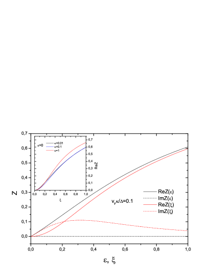
Figure 1: Typical dependencies of $Z(\varepsilon_{n},\xi_{p})$ – factor in one – dimensional FGM with finite correlation lengths: dependences of $Z(\varepsilon_{n}=0,\xi_{p})$ and $Z(\varepsilon_{n},\xi_{p}=0)$ on $\varepsilon_{n}$ and $\xi_{p}$ for $v_{F}\kappa/\Delta=0.1$. At the insert: dependences of $ReZ(\varepsilon_{n}=0,\xi_{p})$ on $\xi_{p}$ for different values of $\kappa$ (in units of $\frac{\Delta}{v_{F}}$). Both $\varepsilon_{n}$ and $\xi_{p}$ are given in units of $\Delta$.

However, the role of finite correlation lengths $\xi$ (finite $\kappa$) is qualitatively similar to static impurity scattering and more detailed calculation shows, that the behavior of $Z$ - factor at small $\epsilon_{n}\ll v_{F}\kappa$ and $|\xi_{p}|\ll v_{F}\kappa$ (with $\varepsilon_{n}>0$) is as follows:

$$Z(\epsilon_{n},\xi_{p})\approx\alpha\left(\frac{v_{F}\kappa}{\Delta}\right)\left(\frac{\epsilon_{n}+i\xi_{p}}{\Delta}\right)\to$$

$$\to 0\quad\mbox{for}\quad\varepsilon_{n}\to 0,\ \xi_{p}\to 0,$$ (26)

with $\alpha(v_{F}\kappa/\Delta)\to 0$ for $\kappa\to 0$, as seen from Fig. 2. In terms of Green’s function this behavior corresponds to:

$$G(\varepsilon_{n},\xi_{p})\approx\frac{1}{\Delta}\alpha\left(\frac{v_{F}\kappa}{\Delta}\right)\frac{\varepsilon_{n}+i\xi_{p}}{i\varepsilon_{n}-\xi_{p}}=-i\frac{1}{\Delta}\alpha\left(\frac{v_{F}\kappa}{\Delta}\right)$$ (27)

Thus, for finite $\kappa$, there is no zero of Green’s function for $\epsilon_{n}=0$ and $\xi_{p}=0$, it remains finite as in impure system.

Figure 2: Dependence of $\alpha\left(\frac{v_{F}\kappa}{\Delta}\right)$ on inverse correlation length.

Vanishing of renormalization factor $Z(\varepsilon_{n},\xi_{p})$ at the “bare” Fermi surface is in correspondence with general topological stability arguments Vol05 – in the absence of static impurity – like scattering the pole singularity of the Green’s function is replaced by zero. In the presence of this additional scattering this zero is replaced by finite discontinuity, i.e. singularity still persists.

III.2 “Hot spots” model in two – dimensions.

In two dimensions we introduce the so called “hot spots” model. Consider typical Fermi surface of electrons moving in the $CuO_{2}$ plane of copper oxides as shown in Fig. 3. If we neglect fine details, the observed (e.g. in ARPES experiments) Fermi surface (and also the spectrum of elementary excitations) in $CuO_{2}$ plane, in the first approximation are described by the usual tight – binding model:

$$\epsilon({\bf p})=-2t(\cos p_{x}a+\cos p_{y}a)-4t^{\prime}\cos p_{x}a\cos p_{y}a$$ (28)

where $t$ is the nearest neighbor transfer integral, while $t^{\prime}$ is the transfer integral between second – nearest neighbors, $a$ is the square lattice constant.

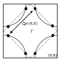
Figure 3: Fermi surface in the Brillouin zone and “hot spots” model. Magnetic zone appears e.g. in the presence of antiferromagnetic long – range order. “Hot spots” correspond to intersections of its borders with Fermi surface and are connected by the scattering vector of the order of ${\bf Q}=(\frac{\pi}{a},\frac{\pi}{a})$.

Phase transition to antiferromagnetic (SDW) state induces lattice period doubling and leads to the appearance of “antiferromagnetic” Brillouin zone in inverse space as is also shown in Fig. 3. If the spectrum of carriers is given by (28) with $t^{\prime}=0$ and we consider the half – filled case, Fermi surface becomes just a square coinciding with the borders of antiferromagnetic zone and we have a complete “nesting” — flat parts of the Fermi surface match each other after the translation by vector of antiferromagnetic ordering ${\bf Q}=(\pm\pi/a,\pm\pi/a)$. In this case and for $T=0$ the electronic spectrum is unstable, energy gap appears everywhere on the Fermi surface and the system becomes insulator, due to the formation of antiferromagnetic spin density wave (SDW). In the case of the Fermi surface shown in Fig.3 the appearance of antiferromagnetic long - range order, in accordance with general rules of the band theory, leads to the appearance of discontinuities of isoenergetic surfaces (e.g. Fermi surface) at crossing points with borders of new (magnetic) Brillouin zone due to gap opening at points connected by vector ${\bf Q}$.

In the most part of underdoped region of cuprate phase diagram antiferromagnetic long – range order is absent, however, a number of experiments support the existence of well developed fluctuations of antiferromagnetic short – range order which scatter electrons with characteristic momentum transfer of the order of ${\bf Q}$. Similar effects may appear due CDW fluctuations. These pseudogap fluctuations are again considered to be static and Gaussian, and characterized by two parameters: amplitude $\Delta$ and correlation length $\xi=\kappa^{-1}$ MS . In this case we can obtain rather complete solution for single – electron Green’s function via summation of all Feynman diagrams of perturbation series, describing scattering by these fluctuations MS ; Sch ; KS . This solution is again exact in the limit of $\xi\to\infty$ Sch , and apparently very close to an exact one in case of finite $\xi$ MS00 . Generalizations of this approach for two – particle properties (vertex – parts) are also quite feasible.

We shall start again with an exact solution for $\xi\to\infty$ (or $\kappa=0$) Sch . First, let us introduce (normal) Green’s function for SDW (CDW) state with long – range order (see e.g. Diagr ):

$$G(\varepsilon_{n},\xi_{\bf p})=\frac{i\varepsilon_{n}-\xi_{\bf p-Q}}{(i\varepsilon_{n}-\xi_{\bf p})(i\varepsilon_{n}-\xi_{\bf p-Q})-W^{2}}$$ (29)

where $W$ denotes the amplitude of SDW (CDW) periodic potential and $\xi_{\bf p}=\varepsilon({\bf p})-\mu$. Then we can write down appropriate $Z$ - factor as:

$$Z(\varepsilon_{n},\xi_{\bf p})=\frac{(i\varepsilon_{n}-\xi_{1})(i\varepsilon_{n}-\xi_{2})}{(i\varepsilon_{n}-\xi_{1})(i\varepsilon_{n}-\xi_{2})-W^{2}}$$ (30)

where we have denoted for brevity: $\xi_{\bf p}=\xi_{1}$ and $\xi_{\bf p-Q}=\xi_{2}$. In the following we shall be mainly interested in the limit of $\varepsilon_{n}\to 0$ and $\xi_{1}\to 0$, i.e. on the approach to the “bare” Fermi surface. Note that $\xi_{2}=0$ defines the so called “shadow” Fermi surface. We have $\xi_{1}=\xi_{2}=0$ precisely at the “hot spots”. In the following it is convenient to introduce a complex variable:

$$z=(i\varepsilon_{n}-\xi_{1})(i\varepsilon_{n}-\xi_{2})$$ (31)

which becomes small for $\varepsilon_{n},\xi_{1},\xi_{2}\to 0$.

III.2.1 Incommensurate combinatorics.

In case of incommensurate (CDW) pseudogap fluctuations, an exact solution for the Green’s function of FGM in the limit of correlation length $\xi\to\infty$ takes the form similar to (20) MS ; Sch and we get (averaging (30) with Rayleigh distribution for W):

$$Z(z)=\int_{0}^{\infty}dW\frac{2W}{\Delta^{2}}e^{-\frac{W^{2}}{\Delta^{2}}}\frac{z}{z-W^{2}}=$$

$$=\int_{0}^{\infty}\frac{d\zeta}{\Delta^{2}}e^{-\frac{\zeta}{\Delta^{2}}}\frac{z}{z-\zeta}=\frac{z}{\Delta^{2}}e^{-\frac{z}{\Delta^{2}}}Ei\left(\frac{z}{\Delta^{2}}\right)$$ (32)

Then, for $z\to 0$ we get:

$$Z(z\to 0)\approx\frac{z}{\Delta^{2}}\left[\ln\left(\gamma^{\prime}\frac{z}{\Delta^{2}}\right)-i\pi\right]$$ (33)

At the “bare” Fermi surface we have $\xi_{1}=0$ and in the following we limit ourselves to $\varepsilon_{n}>0$. Then, from (33) we can easily find limiting behavior of $Z(z)$. Just quoting some results we have:

1. For $\varepsilon_{n}\ll|\xi_{2}|$:

   $$ReZ(\varepsilon_{n}\ll|\xi_{2}|,\xi_{1}=0)\approx\frac{\pi}{2}\frac{\varepsilon_{n}|\xi_{2}|}{\Delta^{2}}$$ (34)

   i.e. “impure” – like linear behavior in $\varepsilon_{n}$.

2. For $\varepsilon_{n}\gg|\xi_{2}|$ (i.e. also at the “hot spot”, where $\xi_{2}=0$):

   $$ReZ(\varepsilon_{n}\gg|\xi_{2}|,\xi_{1}=0)\approx-\frac{\varepsilon_{n}^{2}}{\Delta^{2}}\ln\left(\gamma^{\prime}\frac{\varepsilon_{n}^{2}}{\Delta^{2}}\right)+\frac{1}{2}\frac{\xi_{2}^{2}}{\Delta^{2}}$$ (35)

   i.e. (for $\xi_{2}=0$) NFL behavior similar to one – dimensional case.

Note that we always have $ImZ=0$ for $\xi_{2}=0$, i.e. at the “shadow” Fermi surface and in particular at the “hot spot” itself.

III.2.2 Spin – fermion combinatorics.

Consider now spin – fermion (Heisenberg) model for pseudogap (SDW) fluctuations Sch . In this case we again obtain FGM, but with gap distribution is different (from Rayleigh distribution) and instead of (32) we have:

$$Z(z)=\frac{2}{\sqrt{2\pi}}\int_{0}^{\infty}dW\frac{W^{2}}{\left(\frac{\Delta^{2}}{3}\right)^{3/2}}e^{-\frac{W^{2}}{2\left(\frac{\Delta^{2}}{3}\right)}}\frac{z}{z-W^{2}}=$$

$$=\frac{1}{\sqrt{2\pi}}\int_{0}^{\infty}d\zeta\frac{\sqrt{\zeta}}{\left(\frac{\Delta^{2}}{3}\right)^{3/2}}e^{-\frac{\zeta}{2\left(\frac{\Delta^{2}}{3}\right)}}\frac{\zeta}{z-\zeta}=$$

$$=\frac{\Gamma(3/2)}{\sqrt{2\pi}}\frac{(-z)^{3/2}}{\left(\frac{\Delta^{2}}{3}\right)^{3/2}}\exp\left[-\frac{z}{2\left(\frac{\Delta^{2}}{3}\right)}\right]\Gamma\left(-\frac{1}{2};-\frac{z}{2\left(\frac{\Delta^{2}}{3}\right)}\right)$$

Thus, for $z\to 0$ we obtain:

$$Z(z)\approx\frac{2\Gamma(3/2)}{\sqrt{\pi}}\left[-\frac{z}{2\left(\frac{\Delta^{2}}{3}\right)}+\Gamma(-1/2)\left(-\frac{z}{2\left(\frac{\Delta^{2}}{3}\right)}\right)^{3/2}\right]$$ (36)

Then on “bare” Fermi surface ($\xi_{p}=0$) we have:

$$Z(\varepsilon_{n}\to 0,\xi_{2},\xi_{1}=0)=$$

$$=\frac{2\Gamma(3/2)}{\sqrt{\pi}}\left[-\frac{\varepsilon_{n}(\varepsilon_{n}+i\xi_{2})}{2\left(\frac{\Delta^{2}}{3}\right)}+\right.$$

$$\left.+\Gamma(-1/2)\left(-\frac{\varepsilon_{n}(\varepsilon_{n}+i\xi_{2})}{2\left(\frac{\Delta^{2}}{3}\right)}\right)^{3/2}\right]$$ (37)

In particular, for $\xi_{2}=0$ we have $ImZ=0$ and:

$$Z(\varepsilon_{n}\to 0,\xi_{2}=\xi_{1}=0)=ReZ(\varepsilon_{n}\to 0,\xi_{2}=\xi_{1}=0)=$$

$$=\frac{\Gamma(3/2)}{\sqrt{\pi}}\frac{\varepsilon_{n}^{2}}{\left(\frac{\Delta^{2}}{3}\right)}$$ (38)

so that we obtain quadratic NFL behavior of $Z$ - factor. Again let us present some results on limiting behavior:

1. For $\varepsilon_{n}\ll|\xi_{2}|$:

   $$ReZ(\varepsilon_{n}\ll|\xi_{2}|,\xi_{1}=0)=$$

   $$=\frac{2\Gamma(3/2)}{\sqrt{\pi}}\left[\frac{\varepsilon_{n}^{2}}{2\left(\frac{\Delta^{2}}{3}\right)}+\sqrt{2\pi}\left(\frac{\varepsilon_{n}|\xi_{2}|}{2\left(\frac{\Delta^{2}}{3}\right)}\right)^{3/2}\right]$$ (39)

   i.e. NFL “zero” behavior.

2. For $\varepsilon_{n}\gg|\xi_{2}|$ (i.e. also at the “hot spot” where $\xi_{2}=0$):

   $$ReZ(\varepsilon_{n}\gg\xi_{2},\xi_{1}=0)=\frac{\Gamma(3/2)}{\sqrt{\pi}}\frac{\varepsilon_{n}^{2}}{\left(\frac{\Delta^{2}}{3}\right)}$$ (40)

   i.e. again NFL “zero” behavior.

In the general case of finite correlation lengths $\xi=\kappa^{-1}$ we have to perform numerical analysis using the recursion relations proposed in Refs. Sch ; KS . Again we use the basic definition of $Z$ - factor given in (3). To calculate self – energy $\Sigma(\varepsilon_{n},\xi_{\bf p})$ of an electron moving in the quenched random field of (static) Gaussian spin fluctuations with dominant scattering momentum transfers from the vicinity of characteristic vector ${\bf Q}$, we use the following recursion procedure Sch ; KS which takes into account all Feynman diagrams describing the scattering of electrons by this random field. The desired self–energy is given by

$$\Sigma(\varepsilon_{n},\xi_{\bf p})=\Sigma_{k=1}(\varepsilon_{n},\xi_{\bf p})$$ (41)

with $\xi_{\bf p}=\epsilon({\bf p})-\mu$ (cf. (28)) and

$$\Sigma_{k}(\varepsilon_{n},\xi_{\bf p})=\Delta^{2}\frac{s(k)}{i\varepsilon_{n}+\mu-\epsilon_{k}({\bf p})+inv_{k}\kappa-\Sigma_{k+1}(\varepsilon_{n},\xi_{\bf p})}\;\;.$$ (42)

The quantity $\Delta$ again characterizes the energy scale of pseudogap fluctuations and $\kappa=\xi^{-1}$ is the inverse correlation length of short range SDW fluctuations, $\epsilon_{k}({\bf p})=\epsilon({\bf p+Q})$ and $v_{k}=|v_{\bf p+Q}^{x}|+|v_{\bf p+Q}^{y}|$ for odd $k$ while $\varepsilon_{k}({\bf p})=\varepsilon({\bf p})$ and $v_{k}=|v_{\bf p}^{x}|+|v_{\bf p}^{y}|$ for even $k$. The velocity projections $v_{\bf p}^{x}$ and $v_{\bf p}^{y}$ are determined by usual momentum derivatives of the “bare” electronic energy dispersion $\epsilon({\bf p})$ given by (28). Finally, $s(k)$ represents a combinatorial factor with

$$s(k)=k$$ (43)

for the case of commensurate charge (CDW type) fluctuations with ${\bf Q}=(\pi/a,\pi/a)$ MS79 . For incommensurate CDW fluctuations MS79 one finds

$$s(k)=\left\{\begin{array}[]{cc}\frac{k+1}{2}&\mbox{for odd $k$}\\ \frac{k}{2}&\mbox{for even $k$}.\end{array}\right.$$ (44)

For spin – fermion model of Ref. Sch , the combinatorics of diagrams becomes more complicated. Spin - conserving scattering processes obey commensurate combinatorics, while spin - flip scattering is described by diagrams of incommensurate type (“charged” random field in terms of Ref. Sch ). In this model the recursion relation for the single-particle Green function is again given by (42), but the combinatorial factor $s(n)$ now acquires the following form Sch :

$$s(k)=\left\{\begin{array}[]{cc}\frac{k+2}{3}&\mbox{for odd $k$}\\ \frac{k}{3}&\mbox{for even $k$}.\end{array}\right.$$ (45)

Below we only present our results for spin – fermion combinatorics, as in other cases we obtain more or less similar behavior of renormalization factors.

In Fig. 4 we show the results of numerical calculation of $ReZ(\varepsilon_{n},\xi_{\bf p}=0)$ at different points taken at the “bare” Fermi surface, shown at the insert. For comparison we show data obtained in the limit of infinite correlation length $\xi\to\infty$ (or $\kappa=0$ – exactly solvable case) and for finite $\kappa a=0.01$ (i.e. $\xi=100a$). It is clearly seen that in both cases $ReZ\sim 1$ at “nodal” point $D$, except at very small values of $\varepsilon_{n}$, while in the vicinity of the “hot spot” (points $A$ and $C$), and also at the “hot spot” itself (point $B$), $ReZ$ becomes small in rather wide interval of $\varepsilon_{n}<\Delta$. This corresponds to more or less “Fermi liquid” behavior for “nodal” region (vicinity of Brillouin zone diagonal), with a kind of “marginal” Fermi liquid or Luttinger liquid (NFL) behavior as we move to the vicinity of the “hot spot”.

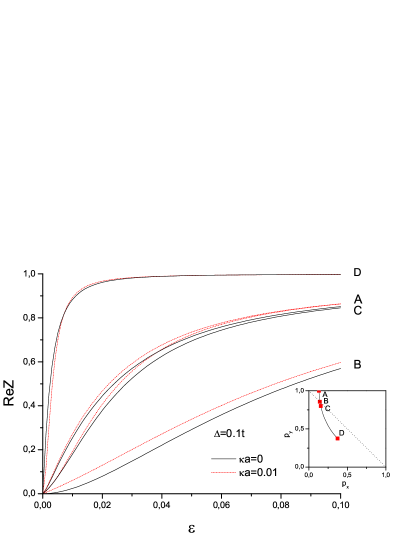
Figure 4: Dependence of $ReZ$ on $\varepsilon_{n}$ (in units of $t$) at different points Fermi surface (corresponding to $t^{\prime}=-0.4t$ and $\mu=-1.3t$) in “hot spots” model (spin – fermion combinatorics of diagrams) with correlation lengths $\xi\to\infty$ $(\kappa=0)$ and $\xi^{-1}a=\kappa a=0.01$. Pseudogap amplitude $\Delta=0.1t$. At the insert we show the “bare” Fermi surface and points, where calculations were done.

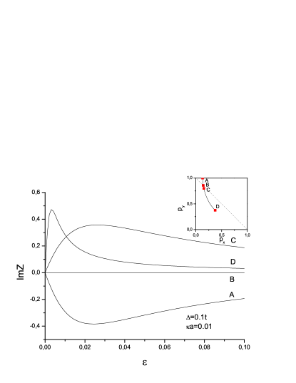
Figure 5: Dependence of $ImZ$ on $\varepsilon_{n}$ (in units of transfer integral $t$) at different points Fermi surface (corresponding to $t^{\prime}=-0.4t$ and $\mu=-1.3t$) in “hot spots” model with finite correlation length $\xi^{-1}a=\kappa a=0.01$ (spin – fermion combinatorics of diagrams). Pseudogap amplitude $\Delta=0.1t$. At the insert — the “bare” Fermi surface and points, where calculations were done.

For completeness in Fig. 5 we show similar comparison of dependences of $ImZ$ on $\varepsilon_{n}$ at the same characteristic points on the Fermi surface and for the same parameters as in Figs. 4. It is only important to stress once again, that only at the “hot spot” itself (point $B$) we have $ImZ=0$, so that $Z$ becomes real, and shows dependence on $\varepsilon_{n}$ more or less equivalent to that proposed for “marginal” Fermi liquids (or Luttinger liquids).

In all cases we observe vanishing of renormalization factor $Z(\varepsilon_{n},\xi_{p})$ at the “bare” Fermi surface. In the absence of static impurity – like scattering due to finite values of correlation length $\xi=\kappa^{-1}$ the pole singularity of the Green’s function is replaced by zero, reflecting topological stability of the “bare” Fermi surface (Luttinger theorem) Vol05 . In the presence of this scattering, singularity of the Green’s function at topologically stable “bare” Fermi surface remains in the form of finite discontinuity.

III.3 Spectral density and Fermi surface “destruction” in “hot spots” model.

Let us return to (29) and perform the usual analytic continuation to real frequencies: $i\varepsilon_{n}\to\varepsilon+i\delta$. Then we obtain:

$$G^{R}(\varepsilon,\xi_{\bf p})=\frac{\varepsilon-\xi_{2}}{(\varepsilon+i\delta-\xi_{1})(\varepsilon-\xi_{2}+i\delta)-W^{2}}=$$

$$=\frac{\varepsilon-\xi_{2}}{(\varepsilon-\xi_{1})(\varepsilon-\xi_{2})-W^{2}+i\delta(2\varepsilon-\xi_{1}-\xi_{2})}$$ (46)

so that spectral density in the case of long – range (CDW,SDW) order has the following form:

$$A_{W}(\varepsilon,\xi_{\bf p})=-\frac{1}{\pi}ImG^{R}(\varepsilon,\xi_{\bf p})=$$

$$=(\varepsilon-\xi_{2})\delta[(\varepsilon-\xi_{1})(\varepsilon-\xi_{2})-W^{2}]sign(2\varepsilon-\xi_{1}-\xi_{2})$$

(47)

Accordingly, for FGM with correlation length $\xi\to\infty$ we have:

$$A(\varepsilon,\xi_{\bf p})=\int_{0}^{\infty}dW{\cal P}_{W}A_{W}(\varepsilon,\xi_{\bf p})$$ (48)

where ${\cal P}_{W}$ is distribution function of gap fluctuations, depending on combinatorics of diagrams and leading to the following separate cases, already considered (or mentioned) above:

III.3.1 Incommensurate combinatorics.

In the case of incommensurate CDW – like pseudogap fluctuations we have:

$${\cal P}_{W}=\frac{2W}{\Delta^{2}}e^{-\frac{W^{2}}{\Delta^{2}}}$$ (49)

– Rayleigh distribution MS74 ; Diagr . Then, from (48) we obtain:

$$A(\varepsilon,\xi_{\bf p})=$$

$$=\frac{\varepsilon-\xi_{2}}{\Delta^{2}}e^{-\frac{(\varepsilon-\xi_{1})(\varepsilon-\xi_{2})}{\Delta^{2}}}\times$$

$$\times\theta[(\varepsilon-\xi_{1})(\varepsilon-\xi_{2})]sign(2\varepsilon-\xi_{1}-\xi_{2})$$

(50)

For $\varepsilon=0$ we have:

$$A(\varepsilon=0,\xi_{\bf p})=\frac{\xi_{2}}{\Delta^{2}}e^{-\frac{\xi_{1}\xi_{2}}{\Delta^{2}}}\theta[\xi_{1}\xi_{2}]sign(\xi_{1}+\xi_{2})$$ (51)

For $\xi_{1}\to\pm 0$ we get:

$$A(\varepsilon=0,\xi_{\bf p}\to\pm 0,\xi_{2})=\pm\frac{\xi_{2}}{\Delta^{2}}\theta(\pm\xi_{2})$$ (52)

so that within the Brillouin zone $A(\varepsilon=0,\xi_{\bf p})$ is nonzero only in the space between “bare” Fermi surface and “shadow” Fermi surface. This qualitative result is confirmed below, for all other combinatorics, for the case of “pure” FGM with $\xi^{-1}=\kappa=0$.

III.3.2 Commensurate combinatorics.

In the case of commensurate CDW – like pseudogap fluctuations we have Wonn :

$${\cal P}_{W}=\frac{1}{\sqrt{2\pi}\Delta}e^{-\frac{W^{2}}{2\Delta^{2}}}$$ (53)

– Gaussian distribution. Then, from (48) we obtain:

$$A(\varepsilon,\xi_{\bf p})=$$

$$=\frac{1}{\sqrt{2\pi}}\frac{\varepsilon-\xi_{2}}{\Delta\sqrt{(\varepsilon-\xi_{1})(\varepsilon-\xi_{2})}}e^{-\frac{(\varepsilon-\xi_{1})(\varepsilon-\xi_{2})}{2\Delta^{2}}}\times$$

$$\times\theta[(\varepsilon-\xi_{1})(\varepsilon-\xi_{2})]sign(2\varepsilon-\xi_{1}-\xi_{2})$$ (54)

with the same qualitative conclusions as in incommensurate case.

III.3.3 Spin – fermion combinatorics.

In the case of SDW – like pseudogap fluctuations of (Heisenberg) spin – fermion model Sch we have gap distribution:

$${\cal P}_{W}=\frac{2}{\pi}\frac{W^{2}}{\left(\frac{\Delta^{2}}{3}\right)^{3/2}}e^{-\frac{W^{2}}{2\left(\frac{\Delta^{2}}{3}\right)}}$$ (55)

Then, from (48) we obtain:

$$A(\varepsilon,\xi_{\bf p})=$$

$$=\frac{1}{\sqrt{2\pi}}\frac{\sqrt{(\varepsilon-\xi_{1})(\varepsilon-\xi_{2})}}{\left(\frac{\Delta^{2}}{3}\right)^{3/2}}e^{-\frac{(\varepsilon-\xi_{1})(\varepsilon-\xi_{2})}{2\left(\frac{\Delta^{2}}{3}\right)}}\times$$

$$\times\theta[(\varepsilon-\xi_{1})(\varepsilon-\xi_{2})]sign(2\varepsilon-\xi_{1}-\xi_{2})$$ (56)

again with the same qualitative conclusions as in incommensurate case.

For the general case of finite correlation lengths $\xi=\kappa^{-1}$ spectral densities can be directly computed using analytic continuation of recursion relations (41), (42) to real frequencies Sch ; KS .

Actually, two – dimensional contour plots of $A(\varepsilon=0,\xi_{\bf p})$ (which are in direct correspondence with ARPES intensity plots) can be used for “practical” definition of renormalized Fermi surface and provide a qualitative picture of its evolution in FGM with the change model parameters.

In Fig. 6 we show typical intensity plots of spectral density $A(\varepsilon=0,\xi_{\bf p})$ in Brillouin zone for the “hot spots” model both for the case of infinite correlation length $\xi^{-1}=\kappa=0$ and for finite (large!) correlation length $\xi^{-1}a=\kappa a=0.01$ (spin – fermion combinatorics of diagrams, in other cases behavior is quite similar) and for different values of pseudogap amplitude $\Delta$. We see that these spectral density plots give rather beautiful qualitative picture of the “destruction” of the Fermi surface in the vicinity of “hot spots” for small values of $\Delta$, with formation of typical “Fermi arcs” as $\Delta$ grows, which is qualitatively resembling typical ARPES data for copper oxides ARPES ; Kord .

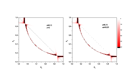
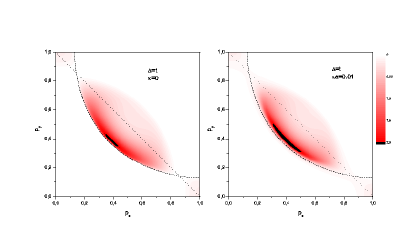
Figure 6: Intensity plots of spectral density $A(\varepsilon=0,\xi_{\bf p})$ in Brillouin zone for the “hot spots” model ($t^{\prime}=-0.4t$ and $\mu=-1.3t$) for the case of infinite correlation length $\xi^{-1}=\kappa=0$ and for finite correlation length $\xi^{-1}a=\kappa a=0.01$ (spin – fermion combinatorics of diagrams) with different values of pseudogap amplitude $\Delta$. “Bare” Fermi surface is shown by dashed line.

III.4 Superconducting $d$ – wave fluctuations.

As we noted above, the case of superconducting $s$ - wave pseudogap fluctuations simply reduces to one – dimensional FGM. Much more interesting is the case of superconducting $d$ - wave fluctuations in $2D$.

To obtain exact results for the case of infinite correlation length $\xi^{-1}=\kappa=0$ we have only to make simple replacements in the above expressions for the “hot spots” model with incommensurate combinatorics: $\xi_{2}\to-\xi_{1}=-\xi_{\bf p}$ and $\Delta\to\Delta_{\bf p}$, where $\Delta_{\bf p}$ defines the amplitude of fluctuations with $d$ - wave symmetry:

$$\Delta_{\bf p}=\frac{1}{2}\Delta\left[\cos(p_{x}a)-\cos(p_{y}a)\right]$$ (57)

with $\Delta$ now characterizing the energy scale of pseudogap fluctuations.

Then (31) reduces to $z=-(\varepsilon_{n}^{2}+\xi_{\bf p}^{2})$ and for $Z$-factor we immediately obtain an expression, similar to (21):

$$Z(\varepsilon_{n},\xi_{p})=$$

$$=-\frac{\varepsilon_{n}^{2}+\xi_{\bf p}^{2}}{\Delta^{2}_{\bf p}}\exp\left({-\frac{\varepsilon_{n}^{2}+\xi_{\bf p}^{2}}{\Delta^{2}_{\bf p}}}\right)Ei\left(-\frac{\varepsilon_{n}^{2}+\xi_{\bf p}^{2}}{\Delta^{2}_{\bf p}}\right)\approx$$

$$\approx-\frac{\varepsilon_{n}^{2}+\xi_{p}^{2}}{\Delta^{2}_{\bf p}}\ln\left(\gamma^{\prime}\frac{\varepsilon_{n}^{2}+\xi_{p}^{2}}{\Delta^{2}_{\bf p}}\right)\to 0$$

$$\quad\mbox{for}\quad\varepsilon_{n}\to 0,\ \xi_{\bf p}\to 0$$ (58)

again replacing the pole singularity by zero at the “bare” Fermi surface, except the “nodal” at the diagonal of the Brillouin zone, where $\Delta_{\bf p}=0$ (cf. (57)).

Instead of (50), we get spectral density as:

$$A(\varepsilon,\xi_{\bf p})=\frac{\varepsilon+\xi_{\bf p}}{\Delta^{2}_{\bf p}}e^{-\frac{\varepsilon^{2}-\xi^{2}_{\bf p}}{\Delta^{2}_{\bf p}}}\theta(\varepsilon^{2}-\xi^{2}_{\bf p})sign\varepsilon$$ (59)

which is nonzero only for $|\xi_{\bf p}|<\varepsilon$. As a result, for $\varepsilon=0$ we have $A(\varepsilon=0,\xi_{\bf p})=0$ for $\Delta_{\bf p}\neq 0$, and it is different from zero only at the intersection of Brillouin zone diagonal with “bare” Fermi surface, where $\Delta_{\bf p}$ given by (57) is zero. At Fermi surface itself we have:

$$A(\varepsilon,\xi_{\bf p}=0)=\frac{|\varepsilon|}{\Delta^{2}_{\bf p}}e^{-\frac{\varepsilon^{2}}{\Delta^{2}_{\bf p}}}$$ (60)

with two maxima at $\varepsilon=\pm\Delta/\sqrt{2}$.

Considering the general case of finite correlation lengths $\xi=\kappa^{-1}$ we again perform numerical analysis using the recursion relations introduced for this problem in Ref. KS , using the basic definition of $Z$ - factor given in (3). To calculate self – energy $\Sigma(\varepsilon_{n},\xi_{\bf p})$ of an electron scattered by static fluctuations of superconducting order parameter with $d$ - wave symmetry, we use the following relation (similar to (42)), sligthly generalizing relations derived in of Ref. KS :

$$\Sigma_{k}(\varepsilon_{n},\xi_{\bf p})=$$

$$=\frac{\Delta^{2}_{\bf p}s(k)}{i\varepsilon_{n}-(-1)^{k}\xi_{\bf p}+ik\kappa(|v^{x}_{\bf p}|+|v^{y}_{\bf p}|)-\Sigma_{k+1}(\varepsilon_{n},\xi_{\bf p})}$$

(61)

where $s(k)$ is defined in (44),

In Fig. 7 we show the results for $ReZ(\varepsilon_{n},\xi_{\bf p}=0)$ again taken at different points of the “bare” Fermi surface, shown at the insert. Correlation length is $\xi=100a$ ($\kappa a=0.01$) and $\Delta=0.1t$. It is clearly seen that $ReZ=1$ precisely at the “nodal” point $D$ (where $\Delta_{\bf p}=0$), but in other point on the “bare” Fermi surface $ReZ$ is strongly renormalized in rather wide intervals of $\varepsilon_{n}<|\Delta_{\bf p}|$, going to zero with $\varepsilon_{n}\to 0$. Thus we again obtain a kind of “marginal” Fermi liquid or Luttinger liquid (NFL), but qualitatively different from the case of “hot spots” model.

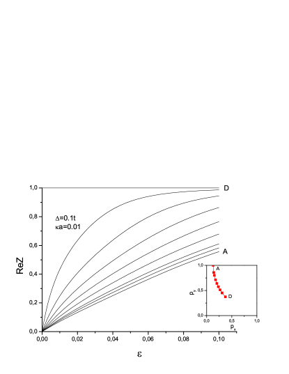
Figure 7: Dependence of $ReZ$ on $\varepsilon_{n}$ (in units of $t$) at different points Fermi surface (corresponding to $t^{\prime}=-0.4t$ and $\mu=-1.3t$) in the model of superconducting ($d$ - wave) pseudpgap fluctuations with correlation length $\xi^{-1}a=\kappa a=0.01$. Pseudogap amplitude $\Delta=0.1t$. At the insert we show the “bare” Fermi surface and points, where calculations were done.

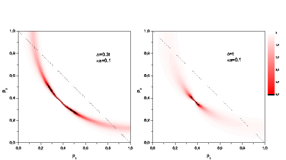
Figure 8: Intensity plots of spectral density $A(\varepsilon=0,\xi_{\bf p})$ in Brillouin zone ($t^{\prime}=-0.4t$ and $\mu=-1.3t$) for the case of superconducting ($d$ - wave) pseudogap fluctuations. Correlation length $\xi^{-1}a=\kappa a=0.1$ (spin – fermion combinatorics of diagrams) for two different values of pseudogap amplitude $\Delta=0.3t$ and $\Delta=t$.

In Fig. 8 we also show typical intensity plots of spectral density $A(\varepsilon=0,\xi_{\bf p})$ in Brillouin zone for the case of superconducting ($d$ - wave) pseudogap fluctuations with correlation length $\xi^{-1}a=\kappa a=0.1$ and two different values of $\Delta$. We see that these spectral density plots give quite different picture of the “destruction” of the Fermi surface in comparison with the case of “hot spots” model, which also, in our opinion, differs significantly from most results of ARPES measurements on copper oxides. Fermi surface is sharply defined only in one point (at the diagonal of the Brillouin zone), where $\Delta_{\bf p}$ given by (57) is precisely zero, and there are no sharply defined Fermi arcs formed close to this point. We observe only some more or less wide “dragon – fly wings” formed around this point. Note also the absence of any signs of “shadow” Fermi surface.

IV Conclusion

We analyzed rather unusual (NFL) behavior of fluctuating gap model (FGM) of pseudogap behavior in both $1D$ and $2D$. We studied in detail quasiparticle renormalization ($Z$ – factor) of the single – electron Green’s function, demonstrating a kind of “marginal” Fermi liquid or Luttinger liquid behavior (i.e. the absence of well – defined quasiparticles close to the Fermi surface) and also the topological stability of the “bare” Fermi surface (Luttinger theorem). This reflects strong renormalization effects leading to the replacement of the usual pole singularity of the Green’s function in Fermi liquid by zero, thus effectively replacing at the Fermi surface of poles by Luttinger surface of zeroes Dz . In the presence of static impurity – like scattering due to the effects of finite correlation lengths of pseudogap fluctuations this singularity is replaced by finite discontinuty.

In $2D$ case we discussed effective picture of Fermi surface “destruction” both in “hot spots” model of dielectric (AFM, CDW) pseudogap fluctuations, as well as for qualitatively different case of superconducting $d$ - wave fluctuations, reflecting NFL spectral density behavior and similar to that observed in ARPES experiments on copper oxides. Intensity plots obtained for the case of AFM (CDW) fluctuations are, in our opinion, more resembling ARPES intensity data obtained in experiments on copper oxides. Note, that this effective picture was also directly generalized for the case of strongly correlated metals or doped Mott insulators KNS using the so called $DMFT+\Sigma_{k}$ approach of Ref. DMFT_S .

Authors are gratefull to G. E. Volovik for his interest and quite useful discussions, which, in fact, initiated this work.

This work was supported in part by RFBR grant 05-02-16301 and programs of the Presidium of the Russian Academy of Sciences (RAS) “Quantum macrophysics” and of the Division of Physical Sciences of the RAS “Strongly correlated electrons in semiconductors, metals, superconductors and magnetic materials”.

References

- (1) M. V. Sadovskii, Usp. Fiz. Nauk 171, 539 (2001) [Physics – Uspekhi 44, 515 (2001)]; ArXiv: cond-mat/0408489
- (2) J. Schmalian, D. Pines, B. Stojkovic, Phys. Rev. B 60, 667 (1999).
- (3) E. Z. Kuchinskii, M. V. Sadovskii, Zh. Eksp. Teor. Fiz. 115, 1765 (1999) [(JETP 88, 347 (1999)]
- (4) M.V.Sadovskii. Zh. Eksp. Teor. Fiz. 66, 1720 (1974) [JETP 39, 845 (1974)]; Fiz. Tverd. Tela 16, 2504 (1974) [Sov. Phys. - Solid State 16, 743 (1974)]
- (5) M. V. Sadovskii, Zh. Eksp. Teor. Fiz. 77, 2070(1979) [Sov.Phys.–JETP 50, 989 (1979)]
- (6) W. Wonneberger, R. Lautenschlager. J.Phys. C 9, 2865 (1976)
- (7) M. V. Sadovskii, A. A. Timofeev. J. Moscow. Phys. Soc. 1, 391 (1991)
- (8) R. H. McKenzie, D. Scarratt. Phys.Rev. 54, R12709 (1996)
- (9) G. E. Volovik. ArXiv: cond-mat/0505089; cond-mat/0601372
- (10) A. B. Migdal. Theory of Finite Fermi Systems and Applications to Atomic Nuclei. Interscience Publishers, NY, 1967; Nauka, Moscow, 1983
- (11) M. V. Sadovskii. Diagrammatics. World Scientific, Singapore 2006
- (12) I. E. Dzyaloshinskii, A. I. Larkin. Zh. Eksp. Teor. Fiz. 65, 411 (1973) [Sov. Phys.–JETP 38, 202 (1974)]
- (13) C. M. Varma, P. B. Littlewood, S. Schmitt-Rink, E. Abrahams, A. E. Ruckenstein. Phys. Rev. Lett. 63, 1996 (1989)
- (14) M. V. Sadovskii, N. A. Strigina. Zh. Eksp. Teor. Fiz. 122, 610 (2002) [JETP 95, 526 (2002)]
- (15) M. V. Sadovskii. Physica C 341-348 , 811 (2000)
- (16) M. R. Norman, H. Ding, M. Randeria, J. C. Campuzano, T. Yokoya, T. Takeuchi, T. Takahashi, T. Mochiku, K. Kadowaki, P. Guptasarma, D. G. Hinks. Nature 392, 157 (1998)
- (17) A. A. Kordyuk, S. V. Borisenko, M. S. Golden, S. Legner, K. A. Nenkov, M. Knupfer, J. Fink, H. Berger, L. Forro, R. Follath. Phys. Rev. B 66, 014502 (2002)
- (18) E. Z. Kuchinskii, I. A. Nekrasov, M. V. Sadovskii. Pis’ma Zh. Eksp. Teor. Fiz. 82, 217 (2005) [JETP Lett. 82, 198 (2005)]
- (19) M. V. Sadovskii, I. A. Nekrasov, E. Z. Kuchinskii, Th. Pruschke, V. I. Anisimov. Phys. Rev. B 72, 155105 (2005)
- (20) I. E. Dzyaloshinskii. Phys. Rev. B 68, 085113 (2003)