Alternating current loss in radially arranged superconducting strips

Abstract

Analytic expressions for alternating current (ac) loss in radially arranged superconducting strips are presented. We adopt the weight-function approach to obtain the field distributions in the critical state model, and we have developed an analytic method to calculate hysteretic ac loss in superconducting strips for small-current amplitude. We present the dependence of the ac loss in radial strips upon the configuration of the strips and upon the number of strips. The results show that behavior of the ac loss of radial strips carrying bidirectional currents differs significantly from that carrying unidirectional currents.

Alternating current (ac) losses are of great importance for electric power applications of superconducting wires. Most of the commonly used high-temperature superconducting wires have tape or strip geometry, and theoretical expressions for hysteretic ac losses for a single superconducting strip have been derived by Norris Norris70 for ac transport currents and by Halse Halse70 for ac magnetic fields, based on the critical state model. Bean62 See also Ref. Brandt93, . Although electromagnetic interaction among multiple strips must be considered in multifilamentary wires and electric power devices, only a few studies have been carried out to derive analytic expressions for ac loss in multiple strips, e.g., in arrays containing an infinite number of strips Mawatari96 or in two coplanar strips. Ainbinder03

In this letter, analytic expressions are derived for ac loss in another type of multiple strips, namely, radially arranged strips. In the radial strips, each superconducting strip has width $a-b$ and thickness $d$ (where $a>b\gg d$ and $a-b\gg d$), and is infinitely long along the $z$ axis. The critical current of each strip is given by $I_{c}=j_{c}d(a-b)$, where $j_{c}$ is the constant critical current density. Bean62 The strips of number $n$ are radially arranged, as shown in Fig. 1. The $k$th strip carries a transport current of $I_{k}$, and we consider the radial strips carrying unidirectional currents (i.e., all strips carry transport currents of identical direction, $I_{k+1}=I_{k}$) and those carrying bidirectional currents (i.e., neighboring strips carry transport currents of opposite directions, $I_{k+1}=-I_{k}$). Radial strips of $n=2$ corresponds to two coplanar strips, as investigated in Refs. Ainbinder03, and Brojeny02, .

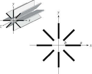
Figure 1: Configuration of radially arranged superconducting strips. The $k$th strip is at $b<\rho<a$ and $\theta=\vartheta_{k}\equiv 2\pi k/n$, and carries a transport current $I_{k}$ [where $\rho=(x^{2}+y^{2})^{1/2}$, $\theta=\arctan(y/x)$, and $k=1,2,\cdots,n$]. Positive integer $n$ denotes the number of strips, and this figure shows an example for $n=8$.

First, we consider radial strips carrying unidirectional currents, and each strip carries a transport current $I_{k}=I_{0}$ (where $I_{k}$ is monotonically increased from $I_{k}=0$ to $I_{k}=I_{0}$) along the $z$ axis. The sheet current in each strip is identical and is denoted by $K_{z}(\rho)$, and the magnetic field component perpendicular to the $k$th strip at $\theta=\vartheta_{k}$ is also identical and is denoted by $H_{\theta}(\rho)$. The Biot-Savart law for radially arranged strips with unidirectional currents is reduced to

$$H_{\theta}(\rho)=\frac{1}{2\pi}\int_{b}^{a}d\varrho K_{z}(\varrho)\frac{n\rho^{n-1}}{\rho^{n}-\varrho^{n}}.$$ (1)

In the ideal Meissner state, the perpendicular magnetic field in the strips is zero. The field distributions (i.e., the sheet current and the perpendicular magnetic field) in the ideal Meissner state are given by $K_{z}(\rho)=K_{M}(\rho;a,b)$ and $H_{\theta}(\rho)=H_{M}(\rho;a,b)$, respectively, and the Meissner distribution functions are given by

$$K_{M}(\rho;u,v) = \begin{cases}2{\cal H}_{0}(\rho;u,v)&\mbox{for }v<\rho<u,\\ 0&\mbox{otherwise,}\end{cases}$$ (2)

$$H_{M}(\rho;u,v) = \begin{cases}-{\cal H}_{0}(\rho;u,v)&\mbox{for }0<\rho<v,\\ 0&\mbox{for }v<\rho<u,\\ {\cal H}_{0}(\rho;u,v)&\mbox{for }\rho>u,\end{cases}$$ (3)

where $u>v>0$ and ${\cal H}_{0}(\rho;u,v)$ is defined by

$${\cal H}_{0}(\rho;u,v)=\frac{I_{0}}{2\pi}\frac{n\rho^{n-1}}{\sqrt{|(\rho^{n}-u^{n})(\rho^{n}-v^{n})|}}.$$ (4)

Equation (2) with (4) corresponds to the current distribution in a strip situated in a wedge-shaped magnetic cavity. Genenko00

In the critical state model, $K_{z}(\rho)$ and $H_{\theta}(\rho)$ satisfy

$$K_{z}(\rho) = j_{c}d\quad\mbox{for }b<\rho<\beta\mbox{ or }\alpha<\rho<a,$$ (5)

$$H_{\theta}(\rho) = 0\hskip 18.00005pt\mbox{for }\beta<\rho<\alpha,$$ (6)

where $\alpha$ and $\beta$ are parameters for the flux front. We adopt the weight-function approach Mikheenko93 to obtain the field distributions; that is, the $K_{z}(\rho)$ and $H_{\theta}(\rho)$ in the critical state model are given as the superposition of the Meissner distribution functions as

$$K_{z}(\rho) = \int_{\alpha}^{a}du\int_{b}^{\beta}dv\,\psi(u,v)K_{M}(\rho;u,v),$$ (7)

$$H_{\theta}(\rho) = \int_{\alpha}^{a}du\int_{b}^{\beta}dv\,\psi(u,v)H_{M}(\rho;u,v),$$ (8)

where $\psi(u,v)$ is the weight function which fulfills

$$\int_{\alpha}^{a}du\int_{b}^{\beta}dv\,\psi(u,v)=1.$$ (9)

Equations (7) and (8) satisfy Eqs. (1) and (6) for any $\psi(u,v)$, and Eq. (9) is necessary to guarantee $I_{0}=\int_{b}^{a}d\rho K_{z}(\rho)$. We obtain $\alpha$, $\beta$, and $\psi(u,v)$ by solving Eqs. (5), (7), and (9).

For a small current of $I_{0}\ll I_{c}$, the flux fronts are close to the edges of the strips, $\alpha\simeq a$ and $\beta\simeq b$, and the weight function can be approximated as

$$\psi(u,v)\simeq\psi_{0}/\sqrt{(a-u)(v-b)},$$ (10)

where $\psi_{0}$ is a constant. Equation (2) with (4) for $\alpha\simeq a$ and $\beta\simeq b$ is reduced to

$$K_{M}(\rho;u,v)\simeq\begin{cases}2\varphi_{b}/\sqrt{\rho-v}&\mbox{for }b<v<\rho<\beta,\\ 2\varphi_{a}/\sqrt{u-\rho}&\mbox{for }\alpha<\rho<u<a,\end{cases}$$ (11)

where the constants $\varphi_{a}$ and $\varphi_{b}$ are defined by

$$\varphi_{a}=\frac{I_{0}}{2\pi}\sqrt{\frac{na^{n-1}}{a^{n}-b^{n}}},\quad\varphi_{b}=\frac{I_{0}}{2\pi}\sqrt{\frac{nb^{n-1}}{a^{n}-b^{n}}}.$$ (12)

Substitution of Eqs. (7), (10), and (11) into Eq. (5) yields

$$j_{c}d\simeq 4\pi\psi_{0}\varphi_{b}\sqrt{a-\alpha},\quad j_{c}d\simeq 4\pi\psi_{0}\varphi_{a}\sqrt{\beta-b}.$$ (13)

The constant $\psi_{0}$ is determined by substituting Eqs. (10) and (13) into Eq. (9), yielding $\psi_{0}=(j_{c}d)^{2}/(4\pi^{2}\varphi_{a}\varphi_{b})$. Equation (13) is thus reduced to

$$a-\alpha\simeq(\pi\varphi_{a}/j_{c}d)^{2},\quad\beta-b\simeq(\pi\varphi_{b}/j_{c}d)^{2}.$$ (14)

Equation (3) with (4) for $\alpha\simeq a$ and $\beta\simeq b$ is reduced to

$$H_{M}(\rho;u,v)\simeq\begin{cases}-\varphi_{b}/\sqrt{v-\rho}&\mbox{for }b<\rho<v<\beta,\\ \varphi_{a}/\sqrt{\rho-u}&\mbox{for }\alpha<u<\rho<a,\end{cases}$$ (15)

and the perpendicular magnetic field near the edges of strips is calculated from Eq. (8) as

$$H_{\theta}(\rho)\simeq\begin{cases}\displaystyle-\frac{j_{c}d}{\pi}\mbox{arctanh}\left(\sqrt{\frac{\beta-\rho}{\beta-b}}\right)&\mbox{for }b<\rho<\beta,\\ \displaystyle\frac{j_{c}d}{\pi}\mbox{arctanh}\left(\sqrt{\frac{\rho-\alpha}{a-\alpha}}\right)&\mbox{for }\alpha<\rho<a.\end{cases}$$ (16)

Here, we consider radial strips carrying unidirectional ac of amplitude $I_{0}$, and the ac loss in radially arranged strips of number $n$ per unit length for one ac cycle is defined by $Q=n\int_{\rm cycle}dt\int_{b}^{a}d\rho E_{z}K_{z}$, where $E_{z}$ is the electric field in the strips. The hysteretic ac loss is calculated from the perpendicular magnetic field given by Eq. (16) for monotonically increased currents as

$$Q = 4n\mu_{0}j_{c}d\left[\int_{\alpha}^{a}d\rho(a-\rho)H_{\theta}(\rho)\right.$$ (17)

$$\left.\qquad\qquad{}-\int_{b}^{\beta}d\rho(\rho-b)H_{\theta}(\rho)\right],$$

and substitution of Eqs. (16) and (14) into Eq. (17) yields

$$Q \simeq \frac{4n}{3\pi}\mu_{0}(j_{c}d)^{2}\Bigl{[}(a-\alpha)^{2}+(\beta-b)^{2}\Bigr{]}$$ (18)

$$\simeq \frac{4\pi^{3}\mu_{0}n}{3(j_{c}d)^{2}}\Bigl{(}\varphi_{a}^{\,4}+\varphi_{b}^{\,4}\Bigr{)}.$$

As seen from Eqs. (11), (15), and (18), the ac loss for small-current limit ($I_{0}\ll I_{c}$) is directly related to the field distributions in the ideal Meissner state. Kajikawa05 The resulting expression for the ac loss in radially arranged strips carrying unidirectional currents is obtained by substituting Eq. (12) into Eq. (18), yielding

$$Q\simeq\frac{\mu_{0}}{6\pi}\frac{I_{0}^{4}}{I_{c}^{2}}\,q_{n}\left(\frac{b}{a}\right),$$ (19)

where $\mu_{0}I_{0}^{4}/6\pi I_{c}^{2}$ corresponds to the ac loss in a single isolated strip Norris70 for $I_{0}\ll I_{c}$, and the geometrical factor $q_{n}(b/a)$ is defined by

$$q_{n}(s)=\frac{n^{3}(1-s)^{2}[1+s^{2(n-1)}]}{2(1-s^{n})^{2}}.$$ (20)

Figure 2 shows the geometrical factor of hysteretic ac loss in radial strips as a function of the parameter $s=b/a$ and $n$. The asymptotic behavior of $q_{n}(s)/n\to 1$ for $s\to 1$ means that electromagnetic interaction between strips can be neglected when the spacing between strips becomes much larger than the width of the strip. The $q_{n}(s)/n$ for unidirectional currents shown in Fig. 2(a) monotonically decreases with increasing $s$, and $q_{n}(s)\to n^{3}/2$ for $s\to 0$ is finite. The $q_{n}(s)/n$ increases with $n$, because the magnetic field near the outer edges at $\rho\sim a$ increases with $n$. For large $n$ (i.e., $s^{n}\ll 1$), Eq. (20) is reduced to $q_{n}(s)\simeq n^{3}(1-s)^{2}/2\propto n^{3}$. The ratio of the ac loss $Q_{b}$ arising from the inner edges at $\rho\simeq b$ to the ac loss $Q_{a}$ arising from the outer edges at $\rho\simeq a$ is given by $Q_{b}/Q_{a}\simeq(\beta-b)^{2}/(a-\alpha)^{2}\simeq(\varphi_{b}/\varphi_{a})^{4}=(b/a)^{2(n-1)}$, thus yielding $Q_{a}\geq Q_{b}$.

Figure 2: Geometrical factor $q_{n}(s)/n$ for ac loss in each strip $Q/n$ as a function of $s=b/a$: (a) $q_{n}(s)/n$ for unidirectional currents and (b) $q_{n}(s)/n$ for bidirectional currents. Inset shows the geometrical factor for total loss $q_{n}(s)$ for bidirectional currents.

Next, we consider radial strips of even number $n$ carrying bidirectional currents; that is, the $k$th strip carries a transport current $I_{k}=(-1)^{k}I_{0}$ along the $z$ axis (where $|I_{k}|$ is monotonically increased from $0$ to $I_{0}$). The sheet current and the perpendicular magnetic field in the $k$th strip at $\theta=\vartheta_{k}$ are given by $(-1)^{k}K_{z}(\rho)$ and $(-1)^{k}H_{\theta}(\rho)$, respectively. The Biot-Savart law for radially arranged strips with bidirectional currents is reduced to

$$H_{\theta}(\rho)=\frac{1}{2\pi}\int_{b}^{a}d\varrho K_{z}(\varrho)\frac{n\rho^{n/2-1}\varrho^{n/2}}{\rho^{n}-\varrho^{n}}.$$ (21)

The field distributions in the ideal Meissner state are given by $K_{z}(\rho)=K_{M}(\rho;a,b)$ and $H_{\theta}(\rho)=H_{M}(\rho;a,b)$, respectively, and the Meissner distribution functions are given by Eqs. (2) and (3), where ${\cal H}_{0}(\rho;u,v)$ for bidirectional currents is defined by

$${\cal H}_{0}(\rho;u,v)=m_{0}(u,v)\frac{\rho^{n/2-1}}{\sqrt{\left|(\rho^{n}-u^{n})(\rho^{n}-v^{n})\right|}},$$ (22)

instead of Eq. (4) for unidirectional currents. The constant $m_{0}(a,b)$ in Eq. (22) is determined such that $I_{0}=\int_{b}^{a}d\rho K_{M}(\rho;a,b)$, and is given by

$$m_{0}(a,b)=\frac{I_{0}\,na^{n/2}}{4\bm{K}(\sqrt{1-b^{n}/a^{n}})},$$ (23)

where $\bm{K}(\kappa)$ is the complete elliptic integral of the first kind.

The calculations of the field distributions and ac loss for bidirectional currents in the critical state model are similar to those for unidirectional currents. Equations (5)–(18) are all valid also for bidirectional currents, except for Eq. (12). Instead, the constants $\varphi_{a}$ and $\varphi_{b}$ for bidirectional currents are defined by

$$\varphi_{a}=\frac{m_{0}(a,b)}{\sqrt{na(a^{n}-b^{n})}},\quad\varphi_{b}=\frac{m_{0}(a,b)}{\sqrt{nb(a^{n}-b^{n})}}.$$ (24)

The ac loss for bidirectional currents can therefore be obtained by substituting Eqs. (23) and (24) into Eq. (18). The resulting expression of ac loss in radially arranged strips carrying bidirectional currents is given by Eq. (19), where the geometrical factor $q_{n}(b/a)$ is given by

$$q_{n}(s)=\frac{\pi^{4}n^{3}(1-s)^{2}(1+s^{2})}{32s^{2}(1-s^{n})^{2}[\bm{K}(\sqrt{1-s^{n}})]^{4}}.$$ (25)

Behavior of the ac loss for bidirectional currents differs significantly from that for unidirectional currents. The $q_{n}(s)$ for bidirectional currents shown in Fig. 2(b) is not a monotonic function of $s$ for $n\geq 6$, whereas $q_{n}(s)$ decreases with increasing $s$ for $n=2$ or $4$. Because the magnetic field tends to be canceled out, loss per strip $q_{n}(s)/n$ decreases with $n$, and even the total loss $q_{n}(s)$ can decrease, as shown in the inset in Fig. 2(b). The elliptic integral in Eq. (25) is reduced to $\bm{K}(\sqrt{1-s^{n}})\simeq\ln(4s^{-n/2})$ for $s^{n}\ll 1$, thus yielding $q_{n}(s)\propto 1/n$ for $n\to\infty$. The $q_{n}(s)\propto s^{-2}[\ln(s)]^{-4}$ diverges when $s\to 0$, because the magnetic field is concentrated near the inner edges at $\rho\sim b$. The ratio of the ac loss arising from the inner edges to the ac loss arising from the outer edges is given by $Q_{b}/Q_{a}\simeq(\varphi_{b}/\varphi_{a})^{4}=(a/b)^{2}$, thus yielding $Q_{a}\leq Q_{b}$.

In summary, we theoretically investigated hysteretic ac loss in radially arranged strips based on the critical state model for small-current limit, $I_{0}\ll I_{c}$. The ac loss in radial strips of unit length for one ac cycle is given by Eq. (19) and the geometrical factor $q_{n}(s)$ is given by Eq. (20) for unidirectional currents or by Eq. (25) for bidirectional currents. The radial strips carrying bidirectional currents have advantages for power application: both leakage magnetic field and ac loss are reduced when the number of strips is large. Such radial strips might be applied to current leads, fault current limiters, and/or cables.Kajikawa06

We gratefully acknowledge M. Furuse, S. Fuchino, and H. Yamasaki for stimulating discussions.

References

• (1) W. T. Norris, J. Phys. D 3, 489 (1970).
• (2) M. R. Halse, J. Phys. D 3, 717 (1970).
• (3) C. P. Bean, Phys. Rev. Lett. 8, 250 (1962); Rev. Mod. Phys. 36, 31 (1964).
• (4) E.H. Brandt, M.V. Indenbom, and A. Forkl, Europhys Lett. 22, 735 (1993); E.H. Brandt and M. Indenbom, Phys. Rev. B48, 12 893 (1993); E. Zeldov, J. R. Clem, M. McElfresh, and M. Darwin, Phys. Rev. B49, 9802 (1994).
• (5) Y. Mawatari, Phys. Rev. B54, 13 215 (1996); K.-H. Müller, Physica C 289, 123 (1997); Y. Mawatari and H. Yamasaki, Appl. Phys. Lett. 75, 406 (1999).
• (6) R. M. Ainbinder and G. M. Maksimova, Supercond. Sci. Technol. 16, 871 (2003).
• (7) A. A. Babaei Brojeny, Y. Mawatari, M. Benkraouda, and J. R. Clem, Supercond. Sci. Technol. 15, 1454 (2002); N. V. Zhelezina and G. M. Maksimova, Tech. Phys. Lett. 28, 618 (2002).
• (8) Yu. A. Genenko, A. Snezhko, and H. C. Freyhardt, Phys. Rev. B62, 3453 (2000).
• (9) P. N. Mikheenko and Yu. E. Kuzovlev, Physica C 204, 229 (1993); J. McDonald and J. R. Clem, Phys. Rev. B53, 8643 (1996).
• (10) K. Kajikawa, T. Hayashi, and K. Funaki, Cryogenics 45, 289 (2005).
• (11) K. Kajikawa, Y. Mawatari, Y. Iiyama, T. Hayashi, K. Enpuku, K. Funaki, M. Furuse, and S. Fuchino, unpublished.