Numerical simulations of a ballistic spin interferometer with Rashba spin-orbital interaction

Abstract

We numerically investigate the transport behavior of a quasi one-dimension (1D) square loop device containing the Rashba spin-orbital interaction in the presence of a magnetic flux. The conductance versus the magnetic field shows the Al’tshuler-Aronov-Spivak (AAS) and Aharonov-Bohm (AB) oscillations. We focus on the oscillatory amplitudes, and find that both of them are strongly dependent on the spin precession angle (i.e. the strength of the spin-orbit interaction) and exhibit no-periodic oscillations, which are well in agreement with a recent experiment by Koga et al. ref8 . However, our numerical results for the ideal 1D square loop device for the node positions of the amplitudes of the AB and AAS oscillations are found to be of some discrepancies comparing with quasi-1D square loop with a finite width. In the presence of disorder and taking the disorder ensemble average, the AB oscillation in the conductance will disappear, while the time-reversal symmetric AAS oscillation still remains. Furthermore, the node positions of the AAS oscillatory amplitude remains the same.

The control over the transport properties of electron spins has gained much attention recentlyref1 ; ref2 ; ref3 . A new sub-discipline of condensed matter physics, spintronics, is emerging rapidly and generating great interests. The promising application of spintronics widely lies in, e.g. information technologyref4 , the spin electron apparatusref5 , and so on. Utilizing the spin orbital (SO) interaction to manipulate the spin degrees of freedoms of electrons has been advanced. Several spin devices have also been theoretically designed. Experimentally, the strength of Rashba SO interaction has successfully been controlled by the applied gate voltage or with some specific design of heterostructures ref6 ; ref7 .

Very recently, Koga et al. used a nanolithographically defined square loop array in the two dimensional electron gases to experimentally demonstrate a gate-controlled electron spin interference ref8 ; addref1 . They observed that the amplitude of the Al’tshuler-Aronov-Spivak (AAS) type oscillation ref9 of the conductance versus the magnetic field $B$ depends strongly on the gate voltage, or the sheet carrier density. This implies that electron spin precession angle $\theta$, caused by the Rashba SO interaction ref10 , is gate-controllable, and can be tuned more than $0.75\pi$. In fact, to experimentally realize a large controllability of the spin precession angle $\theta$ is a very important issue in spintronics, because it is indispensable for realizing some spin devices, e.g. the spin field effect transistor ref5 .

Before the experimental work ref8 , some theoretical works have investigated the transport behavior of a ring with the SO interaction addref2 ; addref3 ; addref4 . In particular, a theoretical prediction of the amplitude of the AAS oscillation has been made by the same group ref11 . Although both the experimental and theoretical results are similar, there are some discrepancies. The theoretical system is an ideal perfect one dimension (1D) square loop with only one terminal contacted outer, for which the backscattering probability was calculated. In the experiment, the device is a quasi-1D square loop (i.e. each arm of the loop has a finite width) with multi terminals, and the transport conductance instead of the backscattering probability was measured. The authors argued that the results for both systems should be similar, however, no through investigation was given. Moreover, in the experimental device, the first order oscillation is the Aharonov-Bohm (AB) oscillation with the period $\phi_{0}$ ($\phi_{0}=h/e$), which is never studied.

In this paper, we numerically simulate the experimental set-up by investigating the amplitude of the AB and the AAS oscillation. We consider a quasi-1D square loop having the Rashba SO interaction (see Fig.1a), which represents one of the cells in the experimental setup by Koga et al. ref8 . The conductance is first calculated from the Landauer-Büttiker formula. Afterwards, by applying the same data analysis process as in the experiment, i.e. the fast Fourier transform (FFT) and the inverse fast Fourier transform (IFFT), the amplitude of the AAS and AB oscillations of conductance are obtained. The numerically calculated node positions of amplitude of AAS oscillation in quasi-1D device are of some departures ($\sim 0.1\pi$) from the theoretical results for the ideal 1D device. The difference is larger for a loop with a wider arm. Moreover, the node positions of the amplitude of the AB oscillation are also studied. Finally, we discuss how the node positions affected by the Dresselhaus SO interaction and the disorder, and find that the Dresselhaus SO interaction can strongly shift the node positions, but the disorder has almost no effect on the node positions.

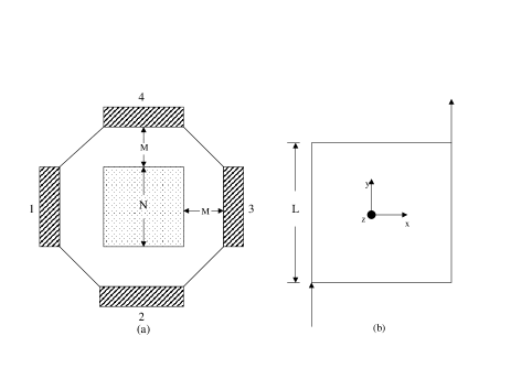
Figure 1: Sketchy illustration for a quasi-1D (a) and an ideal 1D (b) square loop devices. In (a), the potential in the center region is assumed to be very high so that there are no electrons there.

Before investigating the quasi-1D loop system, we first study an ideal 1D square loop model attached with two 1D leads on its two opposite corners (shown in Fig.1b). The goal is to find analytically the node positions of the amplitude of AB or AAS oscillation in the two-terminal system. The Rashba SO interaction exists only in the loop, but absent in the two leads.note11 An incident wave $\psi_{i}$ is splitted at the lower left corner. And the counterclockwise (CCW) and clockwise (CW) wave ballistically travelling along two sides of square loop merge at the right upper corner. $\psi_{o}$ describes the output wave function of the electron at the right upper corner. If only the first order tunneling process is considered, $\psi_{o}$ can be obtained as:

$$\psi_{o}=\frac{1}{2}\left(e^{-i\phi/2}R_{-x}(\theta)R_{y}(\theta)+e^{i\phi/2}R_{y}(\theta)R_{-x}(\theta)\right)\psi_{i}.$$ (1)

where $\phi=2\pi\Phi/\phi_{0}$ with the magnetic flux $\Phi$. The rotation operator $R_{\hat{r}}(\theta)$ is defined as:ref11

$$R_{\hat{r}}(\theta)=\textbf{I}\cos(\theta/2)-i\hat{r}\cdot{\bf\sigma}\sin(\theta/2),$$ (2)

and $\theta=2m^{*}\alpha_{R}L/\hbar^{2}$ is the spin precession angle. Here $L$ is the side length of the 1D square loop and $\alpha_{R}$ is the strength of the Rashba SO interaction. To consider that the incident electron is spin unpolarized, the output probability of the electron is $\overline{<\psi_{o}|\psi_{o}>}$, and it’s given by

$$\overline{<\psi_{o}|\psi_{o}>}=\frac{1}{2}+A(\theta)\cos\phi,$$ (3)

where $A(\theta)=1/4(\sin^{2}\theta+2\cos\theta)$ is the amplitude of the AB oscillation. Then the node positions (marked by $\theta^{*}$) can be obtained easily, and they are $0.636\pi$ and $1.364\pi$, etc. The amplitudes of the higher order oscillation (including the AAS oscillation) are zero here, because the higher order tunnelling process has been neglected in Eq.(1).

Next, we study the model of a quasi-1D square loop sketched in Fig.1a. With the model, no electron exists in the center region of the loop, which can be experimentally realized by the etching technology or the deposited metal split gate. Four leads symbolized as hatched regions in Fig.1a are attached to the four sides of the system. Rashba SO interaction and magnetic field only exist in the quasi loop, and four leads are ideal without SO interaction note11 . The width of the lead is N, the channel width is M, and the side length for the quasi-1D square loop is L=M+N. This quasi-1D model is identical with each cell of the experimental setup in the Ref. ref8 . In their experiment, they applied a square loop array to determine the sheet conductance which is necessary to diminish the AB oscillation and the universal conductance fluctuations.

The Hamiltonian for the quasi-1D model is described as a discrete lattice tight binding model in our numerical calculations. We choose a symmetric gauge and the vector potential $\vec{A}(x,y)=B(-y/2,x/2,0)$, with the lattice spacing as the length unit. Let $a_{j\sigma}$ ($a^{{\dagger}}_{j\sigma}$) be the annihilation (creation) operator of an electron with its spin $\sigma$ at the lattice site $j$, and $a^{{\dagger}}_{j}=(a^{{\dagger}}_{j\uparrow},a^{{\dagger}}_{j\downarrow})$. Then the tight binding model Hamiltonian for the system can be written as:

$$H = -\sum_{j\tau\sigma}(t_{j\tau}a^{{\dagger}}_{j,\sigma}a_{j+\tau,\sigma}+h.c)+\sum_{j\sigma}w_{j}a^{{\dagger}}_{j\sigma}a_{j\sigma}$$ (4)

$$+ \sum_{j}[i\hbar(\lambda_{jx}a^{{\dagger}}_{j}\sigma_{y}a_{j+\hat{x}}-\lambda_{jy}a^{{\dagger}}_{j}\sigma_{x}a_{j+\hat{y}})+h.c.]$$

In the above equation, $\sigma_{x(y)}$ are Pauli matrices, and

$$t_{j\tau} = t\cdot e^{i\frac{e}{\hbar}\vec{A}\cdot\tau},$$ (5)

$$\lambda_{j\tau} = \lambda\cdot e^{i\frac{e}{\hbar}\vec{A}\cdot\tau},$$ (6)

where $t=\frac{\hbar^{2}}{2m^{*}a^{2}}$ is the nearest neighbor hopping element with the lattice space $a$, $\lambda=\frac{\alpha_{R}}{2a}$ describes the strength of the Rashba SO interaction, and $\tau=\pm\hat{x},\pm\hat{y}$. We did not consider the Zeeman splitting energy, because the magnetic field in the experiment is so weak that the Zeeman term is negligibly small compared with other energies, e.g. $t$, the Rashba splitting energy, etc. The disorder potential at each site is not considered right now. Thus we set $w_{j}=0$ in the Hamiltonian as energy zero point. The tight binding Hamiltonian for the ideal 1D square loop system is also given with the same approximations.

The current $I_{p}$ from the lead $p$ ($p=1$, 2, 3, and $4$) flowing into the square loop can be calculated by the Landauer-Büttiker formulaeref12 ; ref13 :

$$I_{p}=\frac{2e^{2}}{h}\sum_{q}T_{pq}(E)[V_{p}-V_{q}].$$ (7)

where $V_{q}$ is the voltage applied on the lead $q$, $T_{pq}(E)$ is the transmission probability from the lead $q$ to the lead $p$, and $E$ is the electron Fermi energy. The temperature is set to be zero, because the thermal energy $k_{B}T$ is much smaller than the other energy scales in the experiment. The transmission probability $T_{pq}$ is determined by $T_{pq}=Tr[\Gamma_{p}G^{R}\Gamma_{q}G^{A}]$ ref14 ; ref15 . Here $\Gamma_{p}=i[\Sigma^{R}_{p}-\Sigma^{A}_{p}]$, and $G^{R(A)}(E)$ is the retarded (advanced) Green function given by:

$$G^{R}(E)=(G^{A}(E))^{\dagger}=\frac{1}{E-H_{c}-\sum\limits_{p=1}^{4}\Sigma^{R}_{p}},$$ (8)

where $\Sigma_{p}^{R(A)}$ is the retarded (advanced) self-energy of lead $p$ and $H_{c}$ is the single particle Hamiltonian given by Eq. (4) for the isolated finite-size system at the center. In the following numerical calculations, the lead’s voltages $V_{p}$ are set as: $V_{1}=V/2$ and $V_{3}=-V/2$, i.e. a longitudinal bias is added in the $x$ direction. The transverse lead-2 and lead-4 act as the voltage probes, and their voltages $V_{2}$ and $V_{4}$ are calculated from the condition $I_{2}=I_{4}=0$. Finally, the longitudinal conductance $\sigma$ is obtained as: $\sigma=I_{1}/V=-I_{3}/V$. In the numerical calculations, we let $t=1$ to be the energy unit.

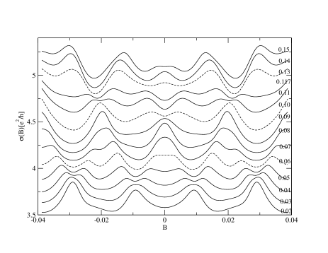
Figure 2: The longitudinal conductance $\sigma(B)$ versus the magnetic field $B$ for the quasi-1D device at different Rashba interaction $\lambda$, with the parameters $N=12$, $M=6$, and the Fermi energy $E=-2.0$. The value of $\lambda$ is indicated with each curve. B is in the unit of $\frac{a^{2}e}{\hbar}$. The plotted curves are shifted along the y-axis for comparison.

The longitudinal conductance $\sigma$ of the quasi-1D square loop system with N=12 and M=6 versus magnetic field $B$ at different spin orbital interaction $\lambda$ are shown in Fig.2. These conductance curves clearly exhibit the existence of the AB oscillation with the period $\phi_{0}$ and the AAS oscillation with the period $\phi_{0}/2$. Since each arm of the loop has a certain width, these oscillations are not exactly periodic. Their oscillatory amplitudes at $B=0$ can be figured out by using the FFT. From the graph, we also find the alternative changing of peak and dip feature in $\sigma(B)$ at B=0 with increasing of the Rashba interaction. This phenomenon is consistent with the experimental results ref8 .

Then for each curve of the conductance in Fig.2 with a fixed value of the Rashba strength $\lambda$, we can employ the FFT and IFFT techniques to extract out the amplitudes of the AB and AAS oscillations at zero magnetic field. The data analysis is identical with the experimental procedure. Since $\lambda=\frac{\alpha_{R}}{2a}$ and $t=\frac{\hbar^{2}}{2m^{*}a^{2}}$, the Rashba strength $\lambda$ and the spin precession angle $\theta$ is related by $\theta=\frac{2L}{at}\lambda$. Fig.3 shows the amplitudes $\sigma(B=0)$ of the AB and the AAS oscillations at $B=0$ versus the spin precession angle $\theta$ for different sizes of the device. The node positions $\theta^{*}$ for both AB and AAS oscillations are indicated in each graph. For comparison, the amplitudes of the AB and the AAS oscillations of the exact 1D square loop system (see Fig.1b) are also calculated by using the tight binding model and the Landauer-Büttiker formulae, in which the higher order processions and the reflecting processions have all been included (see Fig.4).

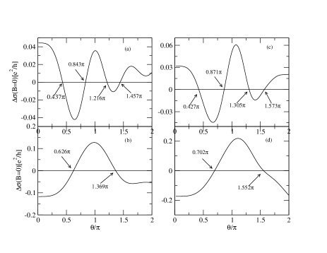
Figure 3: Numerical results for the amplitude of the AAS (a and c) and the AB (b and d) oscillations at B=0 of quasi-1D square loop system versus spin precession angle $\theta$. The system size is N=12, M=6 for part (a), (b), and N=20, M=10 for part (c), (d). The $\theta$ values of node positions are indicated in each graph. The electron Fermi energy is E = -2.0.

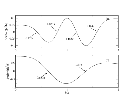
Figure 4: Numerical results for the amplitude of the AAS (a) and the AB (b) oscillations at B=0 in an ideal 1D square loop system versus spin precession angle $\theta$ with L=30. The $\theta$ values of node positions are indicated in the figure. The electron Fermi energy is E =-1.7.

For the ideal 1D system, the numerical results exhibit that the node positions $\theta^{*}$ of the amplitude of the AAS oscillation are $0.420\pi,0.821\pi,1.183\pi,1.584\pi$ etc (see Fig.4a), and $\theta^{*}$ for the AB oscillation are $0.637\pi$ and $1.371\pi$, etc (see Fig.4b). These values are calculated at electron Fermi energy $E=-1.7$, which is close to the bottom of the band. Because near the band bottom, the energy momentum dispersion relation is almost quadratic, and the spin precession angle $\theta$ is independent with $E$. So the node positions of $\theta$ remain unchanged even at different Fermi levels $E$. These node positions are in agreement with the previous theoretical resultsref11 or the Eq.(3) for the ballistic system, and the errors are within $0.01\pi$ for all node positions $\theta^{*}$. This means that the higher order tunneling processions (e.g. electron goes around the loop multi-times) and the reflecting processions have limited effect on the node positions $\theta^{*}$. Furthermore, our numerical calculations also find that so long as the lengths of CW and CCW paths are the same, the conductance is identical no matter where the leads are connected to the perimeter of the loop ref11 .

Next, let us discuss the numerical results of the quasi-1D system (shown in Fig.3). The amplitudes $\Delta\sigma(B=0)$ of the AB and AAS oscillations are oscillatory functions of the spin precession angle $\theta$, which are similar with the ideal 1D device. Moreover, it also clearly shows that $\Delta\sigma(B=0)$ is not a periodic function. This is contrast to an ideal 1D device. In that case, $\Delta\sigma(B=0)$ versus $\theta$ is approximately a periodic function with the period $\pi$ for the AAS amplitude and $2\pi$ for the AB amplitude, like $A(\theta)$ in previous theoretical calculation ref11 and Eq.(3) in this paper. But this fact is consistent with the experimental results ref8 .

Following, we focus on the node positions $\theta^{*}$ of the oscillatory amplitudes, which have been given in Fig.3. These values of $\theta^{*}$ have quite large difference with an ideal 1D system, and the errors can be more than $0.1\pi$. For a loop with wider arm, the discrepancy is larger. For example, for the arm’s width $M=10$, the second node position $\theta^{*}$ of the AB oscillation is at $1.552\pi$ (see Fig.3d), which has an error of $0.188\pi$ with the corresponding value $1.364\pi$ of the ideal 1D device.

Therefore, we need to emphasize that if the width of the loop arm in the device by Koga et al. has been taken into account, then the node positions $\theta^{*}$ deviate from the ones for the ideal 1D device. However, their experimental conclusion, that the spin precession angle $\theta$ due to the Rashba SO interaction is gate-controllable, remains valid. Furthermore the tunable range of $\theta$ could be much larger than the value stated in their paper since the node positions $\theta^{*}$ have larger deviations for quasi-1D devices.

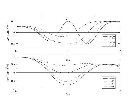
Figure 5: Numerical results for the amplitude of the AAS (a) and the AB (b) oscillations at B=0 of an ideal 1D square loop system versus Rashba dependent spin precession angle $\theta$ with L=30. r is the ratio of Dresselhaus versus Rashba interaction strength with $r\equiv\alpha_{D}/\alpha_{R}$. The Fermi energy is E=-1.7.

Up to now, we only consider the existence of the Rashba SO interaction in the loop, and the Dresselhaus SO interaction has been neglected. If there exists both Rashba and Dresselhaus SO interactions, how are the node positions $\theta^{*}$ affected? In fact, the 1D loop having two kinds of SO interactions has been investigated by a very recent theoretical work by Ramaglia et al.ref18 . Their results show that Dresselhaus SO interaction strongly shifts the nodes of Rashba-dependent transmission in an ideal 1D model. Here we further investigate the ideal 1D system with these two kinds of SO interaction. The tight binding Hamiltonian of Dresselhaus SO interaction is given as:

$$H_{D}=\sum_{j}[i\hbar(\beta_{jy}a^{{\dagger}}_{j}\sigma_{y}a_{j+\hat{y}}-\beta_{jx}a^{{\dagger}}_{j}\sigma_{x}a_{j+\hat{x}})+h.c.]$$ (9)

where $\beta_{j\tau}=\beta\cdot e^{i\frac{e}{\hbar}\vec{A}\cdot\tau}$, $\beta=\alpha_{D}/2a$, and $\alpha_{D}$ is the strength of Dresselhaus SO interaction. The total Hamiltonian in the present system is the Hamiltonian in Eq.(4) plus $H_{D}$. Then the amplitude of AAS and AB oscillation can be solved by the same method as in the above.

In Fig. (5), we present the results of the amplitudes of AAS and AB oscillations at B=0 for the exact 1D quare loop system as a function of Rashba spin precession angle $\theta$ at different values of Dresselhaus interaction. In this graph we could clearly see that with the increasing of Dresselhaus SO interaction, the node positions will not only vary, even the number of nodes may change. For example in Fig. (5a), the number of nodes will decrease from 4 to 3 at $r=0.2$ ($r\equiv\alpha_{D}/\alpha_{R}$), and further to 2 at $r>0.2$. The same situation also happens in the AB oscillation amplitude. These results are consistent with the analytical results ref18 . Therefore, if both SO interactions are presented in the system, using node positions to determine the Rashba SO interaction strength is not very reliable. However, from the oscillation of the amplitude AAS or AB versus the gate voltage, it still clearly indicates that the strength of SO interaction can be well tuned.

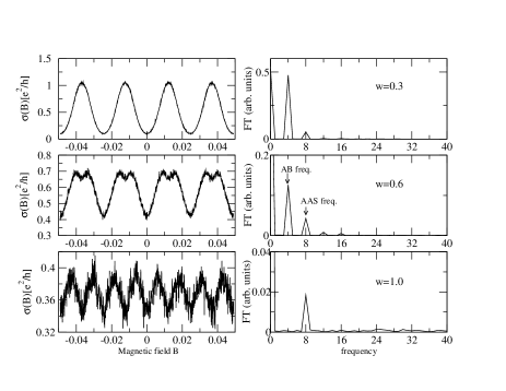
Figure 6: Left panel: ensemble averaged conductance as a function of magnetic field B at different disorder strength of the exact 1D square loop system. Right panel: the corresponding Fourier transform spectra of the conductance. The location of AB frequency and AAS frequency is indicated in the graph. The parameters are the Fermi energy E=-1.7, the system size L=16, and the Rashba interaction $\lambda=0.1$.

Finally, we study how the node positions $\theta^{*}$ are affected by the ensemble average. Notice that the device in the experiment by Koga et al. is a square loop array, not a single square loopref8 . So the ensemble average has to be investigated in order to make a direct comparison with the experimental results. The various ensemble averaging procedures have been studied in investigating the persistent current in a closed mesoscopic ring about ten years ago. Those include taking the ensemble average on the number of particle, on the chemical potential, or on the disorder addref5 ; addref6 . The present square loop array is an open system, its chemical potential is determined by the leads, but the disorder structure for each individual loop is random. When giving the disorder structure and the chemical potential, the number of electrons in the loop is fixed and its value can be non-integer in an open system. So in the following we take the average over the disorder ensembleaddref6 . To consider the existence of the disorder, the random lattice on site energy $w_{j}$ in Eq. (4) is generated by an uniformly distribution $[-w/2,w/2]$ with disorder strength $w$. All these conductance curves are averaged over up to 2000 disorder realizations at $w\neq 0$. The conductance as a function of magnetic field B at different disorder strength $w$ are shown in Fig. (6) left panel, with their corresponding FT (Fourier transform) spectra on the right panel. With the increasing of disorder strength, both the conductance and the conductance oscillation amplitude will decrease. This is due to the fact that the electron will be localized at large disorder strength. In particular, in the strong disorder case, AB oscillation will disappear, but AAS oscillation still exists even at the disorder strength $w=1.0$, because the AAS oscillation is the interference between two time reversal pathes and it is independent of the disorder structure. These results are in agreement with the experimental results and the previous theoretical predictionsref8 ; ref11 .

Next, we focus on the node positions $\theta^{*}$ after the disorder ensemble average. Fig.7 shows the ensemble averaged AAS oscillation amplitude at B=0 of an ideal 1D loop model at different disorder strength $w$. $w=0$ is not shown in the graph, because in that case the oscillation amplitude is much larger than $w=0.6$ or $w=1.0$. It is clear that both the node positions of $\theta$ and the oscillation shape is unchanged versus disorder. These graphs demonstrate that with a little strong spin-independent disorder and ensemble average, the AB oscillation will disappear in the conductance. Meanwhile, the node positions $\theta^{*}$ of AAS oscillation amplitude still remains the same.

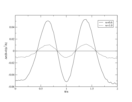
Figure 7: The amplitude of the AAS oscillation at B=0 of an ideal 1D square loop system versus Rashba dependent spin precession angle $\theta$ with L=20. The node positions are identical compared with no disorder. The electron Fermi energy is E=-1.7.

In summary, by using the tight binding model and the Landauer-Büttiker formula, we numerically study the electron transport through a quasi one dimensional square loop with the Rashba spin-orbit interaction. The conductance $\sigma$ as a function of the magnetic field $B$ is obtained, and exhibits the Al’tshuler-Aronov-Spivak (AAS) and Aharonov-Bohm (AB) oscillations. These oscillatory amplitudes are non-periodic with the Rashba spin precession angle $\theta$. These results are in agreement with the recent experiment by Koga et al. ref8 . To compare with an ideal 1D square loop device, the node positions of the amplitudes of the AB and AAS oscillations have some deviations. For a loop with a wider arm, the deviations can be quite large. When under the influence of spin-independent disorder and ensemble average, the AB oscillation will disappear and only AAS oscillation survives in the conductance. In particular, the node positions of the AAS oscillatory amplitude are almost unchanged.

Acknowledgments: We gratefully acknowledge financial support from US-DOE under Grant No. DE-FG02-04ER46124 and NSF CCF-0524673. QFS is supported by NSF-China under Grant Nos. 90303016, 10474125, and 10525418. BC is supported by NSF-China under Grant Nos. 10574035 and 10274070.

References

- (1) G. A. Prinz, Science 282, 1660 (1998).
- (2) S. A. Wolf, D. D. Awschalom, R. A. Buhrman, J. M. Daughton, S. von Molnar, M. L. Roukes, A. Y. Chtchelkanova, and D. M. Treger, Science 294, 1488 (2001).
- (3) D. Awschalom, D. Loss, and N. Samarth (.eds.), Semiconductor Spintronics and Quantum Computation (Springer, Berlin, 2002).
- (4) D. Loss and D. P. DiVincenzo, Phys. Rev. A. 57, 120 (1998).
- (5) S. Datta and B. Das, Appl. Phys. Lett. 56, 665 (1990).
- (6) J. Nitta, T. Akazaki, H. Takayanagi, and T. Enoki, Phys. Rev. Lett. 78, 1335 (1997).
- (7) T. Koga, J. Nitta, T. Akazaki, and H. Takayanagi, Phys. Rev. Lett. 89, 046801 (2002).
- (8) T. Koga, Y. Sekine, and J. Nitta, cond-mat/0504743 (2005).
- (9) T. Bergsten, T. Kobayashi, Y. Sekine, and J. Nitta, cond-mat/0512264 (2005).
- (10) B. L. Al’shuler, A. G. Aronov, and B. Z. Spivak, JETP Lett. 33, 94 (1981).
- (11) E. I. Rashba, Sov. Phys. Solid State 2, 1109 (1960).
- (12) J. Nitta, F.E. Meijer, and H. Takayanagi, Appl. Phys. Lett. 75, 695 (1999).
- (13) D. Bercioux, M. Governale, V. Cataudella and V. M. Ramaglia, Phys. Rev. Lett. 93, 056802 (2004).
- (14) S. Souma and B. K. Nikolic, Phys. Rev. B. 70, 195346 (2004).
- (15) T. Koga, J. Nitta, and M. van Veenhuizen, Phys. Rev. B 70, 161302(R) (2004).
- (16) Here we consider that the Rashaba SO interaction only exists in the loop and the leads are assumed to be without SO interaction. In fact, if the leads have the SO interaction, our results, in particular the node positions , keep similar, because the phase of the electron travelling through the loop is identical regardless of the leads with or without the SO interaction.
- (17) S. Datta, Electronic Transport in Mesoscopic Systems (Cambridge University Press, Cambridge, 1995).
- (18) M. Büttiker, Phys. Rev. Lett. 57, 1761 (1986).
- (19) R. Landauer, Philos. Mag. 21, 863 (1970).
- (20) Y. Meir and N. S. Wingreen, Phys. Rev. Lett. 68, 2512 (1992).
- (21) V. M. Ramaglia, V. Cataudella, G. DeFilippis, and C. A. Perroni, Phys. Rev. B. 73, 155328 (2006).
- (22) H.-F. Cheung, E.K. Riedel, and Y. Gefen, Phys. Rev. Lett. 62, 587 (1989); G. Montambaux, H. Bouchiat, D. Sigeti, and R. Friesner, Phys. Rev. B 42, 7647 (1990); F. von Oppen and E.K. Riedel, Phys. Rev. Lett. 66, 84 (1991).
- (23) B.L. Altshuler, Y. Gefen, and Y. Imry, Phys. Rev. Lett. 66, 88 (1991).