Physical meaning and measurement of the entropic parameter $q$ in an inhomogeneous magnetic systems

Abstract

In this paper we present a thorough analysis of two systems magnetically inhomogeneous: the manganite La_0.7Sr_0.3MnO₃/MgO and the amorphous alloy Cu₉₀Co₁₀. In both cases, the non-extensive statistics yield a faithful description of the magnetic behavior of the systems. In the model proposed here, the inhomogeneous magnetic system is composed by many Maxwell-Boltzmann homogeneous bits and the entropic parameter $q$ is related to the moments of the distribution of the inhomogeneous quantity. From the analysis of Scanning Tunnelling Spectroscopy (STS) images, the $q$ parameter can be directly measured.

I Introduction

Tsallis thermostatistics has been widely used in a number of different contextsweb . The framework is applicable to systems which, broadly speaking, present at least one of the following properties: (i) long-range interactions, (ii) long-time memory, (iii) fractality and (iv) intrinsic inhomogeneity web ; Tsallis (2001). Manganese oxides, or simply manganites, seems to embody three out of these four ingredients: they present Coulomb long-range interactions Lorenzana et al. (2001a, b); Moreo et al. (1999), clusters with fractal shapes Dagotto et al. (2001); Ausloos et al. (2002) and intrinsic inhomogeneity Dagotto et al. (2001); Dagotto (2003); Becker et al. (2002); Kumar and Majumdar (2004); Ahn et al. (2004). Indeed, in a sequence of previous publications Reis et al. (2002a, b, 2003), it has been shown that the magnetic properties of manganites can be properly described within a mean-field approximation using Tsallis statistics.

II PHYSICAL PICTURE

We consider an inhomogeneous magnetic system composed by many homogeneous parts (clusters) with different sizes, each one of them described by the Maxwell-Boltzmann statistics. By averaging the magnetization over the whole system, we recover the Tsallis non-extensivity. A relationship between the $q$ parameter and the moments of the distribution is obtained. The model is tested using Scanning Tunnelling Spectroscopy (STS) conductance maps, where the $q$ parameter could be obtained and, consequently, the bulk magnetization predicted. We also apply the results to describe the magnetic behavior of Cu₉₀Co₁₀ amorphous ribbons.

The starting point is a magnetic system formed by small regions, or clusters of Maxwell-Boltzmann bits, each one of them with magnetization $\mathcal{M}(\mu,T,H)$ given by the usual Langevin functionGuimar es (1998):

$$\mathcal{M}(\mu,T,H)=\mu\left[\coth x-\frac{1}{x}\right]$$ (1)

where $x=\mu H/kT$. The clusters are distributed in size, and therefore in their net magnetic moment. Let $f(\mu)$ be the distribution of the clusters magnetic moment. Thus, the average magnetization of the sample will be given by:

$$\langle\mathcal{M}\rangle=\int_{0}^{\infty}\mathcal{M}(\mu,T,H)f(\mu)d\mu$$ (2)

On the other hand, Ref. Reis et al. (2003); com shows that the non-extensive magnetization is given by the generalized Langevin function:

$$\mathcal{M}_{q}=\frac{\mu_{ne}}{(2-q)}\left[\coth_{q}x-\frac{1}{x}\right]$$ (3)

where $q\in\Re$ is the Tsallis entropic parameter and $x=\mu_{ne}H/kT$.

Equating the susceptibilities

$$\chi_{q}=\langle\chi\rangle\equiv\lim_{H\rightarrow 0}\frac{\partial M}{\partial H}$$ (4)

and the saturation values ($H\rightarrow\infty$) of Eqs. 2 and 3, we find a analytical expression to the $q$ parameter:

$$q(2-q)^{2}=\frac{\langle\mu^{2}\rangle}{\langle\mu\rangle^{2}}$$ (5)

where $\langle\mu\rangle$ and $\langle\mu^{2}\rangle$ are the first and second moments of the distribution $f(\mu)$, respectively. This result is valid for any $f(\mu)$, and is analogous to that obtained by Beck Beck (2001) and Beck and Cohen Beck and Cohen (2003).

Now, let us consider a distribution of critical temperatures. Again, the magnetization of a small region is given by the usual Langevin function (Eq.1), however, within the mean-field approximation, where:

$$x=\frac{\mu(H_{0}+\lambda\mathcal{M})}{kT}$$ (6)

and $\lambda=3kT_{C}/\mu^{2}$ corresponds to the mean-field parameter. Unfortunately, considering a distribution of critical temperatures, the average magnetization

$$\langle\mathcal{M}\rangle=\int_{0}^{\infty}\mathcal{M}(\mu,T,H_{0},T_{C},\mathcal{M})f(T_{C})dT_{C}$$ (7)

can not be reduced in a similar fashion to what was done in the case of a distribution of magnetic moments. Thus, a closed and simple expression connecting the $q$ parameter and the moments of the distribution of critical temperatures could not be obtained. However, as will be discussed, the connection with experimental results will provide some suggestions.

III Connections with experimental results

III.1 Distribution of magnetic moments

As discussed before, the $q$ parameter is related to the moments of the distribution of magnetic moments (Eq. 5). Thus, to measure the entropic parameter we need to measure, a priori, the distribution of magnetic moments. Below, we will discuss how to extract $f(\mu)$ from some experimental data.

III.1.1 Manganites

Colossal magnetoresistance (CMR) effectDagotto (2003), usually observed on manganites, has been proposed in terms of intrinsic inhomogeneitiesDagotto (2003); Dagotto et al. (2001); Becker et al. (2002), which can lead to a formation of insulating and conducting domains within a single sample, i.e., electronic phase separation in a chemical homogeneous sample. The inhomogeneities alter the local electronic and magnetic properties of the sample and should therefore be visible via STS Renner et al. (2002); Fath et al. (1999); Becker et al. (2002) or Magnetic Force Microscopy (MFM) Lu et al. (1997); Zhang et al. (2002).

Becker and co-workersBecker et al. (2002) measured STS in a La_0.7Sr_0.3MnO₃/MgO thin film and visualized a domain structure of conducting (ferromagnetic) and insulating (paramagnetic) regions with nanometric size, since this manganite has a transition from a metallic phase (below T_C) to an insulating phase (above T_C), with a strong phase coexistence/competition around T${}_{C}\sim$ 330 K. These STS conductance maps obtained by those authors at 87 K, 150 K and 278 K are reproduced in figure 1(a). From these 1-bit images (black regions mean insulating/paramagentic phase and white regions stand for conducting/ferromagnetic phase), it was possible to determine the distribution of clusters size. Considering that the cluster size $\phi$, measured in pixels, is proportional to the magnetic moment $\mu$ of the cluster, Eq. 5 can be re-written as:

$$\frac{\langle\phi^{2}\rangle}{\langle\phi\rangle^{2}}=\frac{\langle\mu^{2}\rangle}{\langle\mu\rangle^{2}}=q(2-q)^{2}$$ (8)

The conductance map at 278 K has a distribution of clusters as presented in figure 1(a), and, using Eq. 8 we obtained from the data $q=$2.95.

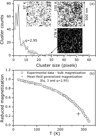
Figure 1: (a) Scanning tunnelling spectroscopy images obtained at different temperatures on La_0.7Sr_0.3MnO₃/MgO manganite thin film, after Becker et al.Becker et al. (2002). White regions are conducting (ferromagnetic phase) clusters and the black regions are insulating clusters (paramagnetic phase). The main graphic is the cluster size distribution of the image at 278 K, proportional to the cluster magnetic moment distribution, where, using Eq.8, $q=2.95$ could be directly obtained. (b) Using the mean-field (reduced) generalized magnetization (Eq.3: $+$ symbol), we could predict the bulk magnetization, in a satisfactory agreement with the measured one ($\circ$ symbol), in a reduced scale $\mathcal{M}/\mathcal{M}$(18 K)Becker et al. (2002).

With this value of $q$, the total magnetization of the system can be predicted, by considering the mean-field approximation into the generalized magnetization (Eq.3), where $x=3m_{q}/t$, $m_{q}=\mathcal{M}_{q}/\mu_{ne}$, $t=T/T_{C}^{(1)}$ and $T_{C}^{(1)}=298K$Reis et al. (2002a) (see refs. Reis et al. (2003, 2002a) for details concerning the mean-field approximation applied to the non-extensive magnetization). This procedure results in a satisfactory agreement between the predicted reduced magnetization ($m_{q}=$0.25; the $+$ symbol) and the experimental one (the $\circ$ symbol), obtained measuring the bulk magnetizationBecker et al. (2002), as presented in figure 1(b). The images at 87 K and 150 K were not analyzed, since the clusters have already percolated.

The procedure above described shows how to extract the $q$ parameter from an experimental data, and then how to apply the obtained $q$ parameter to predict macroscopic quantities of the system. In addition, these results exemplify the relation between non-extensivity and microscopic inhomogeneities. Finally, it is important to stress that $q$ is related to the dynamics of the system, since it measures the distribution of magnetic moments, that contains the dynamics.

III.1.2 Granular Alloys

Ferrari and co-workersFerrari et al. (1997) analyzed some melt-spun Cu₉₀Co₁₀ ribbons, materials intrinsically inhomogeneousMurillo et al. (2004); Panissod et al. (2001). They considered Eq.2 to study the magnetic behavior of these materials, supposing a Log-Normal distribution of magnetic moments:

$$f(\mu)=\frac{1}{\sqrt{2\pi}\;s\;\mu}\;\exp\left[-\frac{\ln^{2}(\mu/\mu_{0})}{2\;s^{2}}\right]$$ (9)

where the k^th moment is $\langle\mu^{k}\rangle=\mu_{0}^{k}\exp(k^{2}s^{2}/2)$.

Those authors used this model to fit the magnetization curves at room temperature, as displayed in figure 2-top. The fitting parameters for the sample (a) are $\mu_{0}=500\mu_{B}$ and $s=1.16$; and for the sample (b), $\mu_{0}=3900\mu_{B}$ and $s=0.93$. Both samples are Cu₉₀Co₁₀, however, prepared under different conditionsFerrari et al. (1997). With these values and using Eqs.9 and 5, we could obtain the $q$ parameter for both samples: (a) $q=3.11$ and (b) $q=2.90$.

With those values of $q$, the non-extensive magnetic susceptibility was obtained:

$$\chi_{q}=\frac{q\mu_{ne}^{2}}{3kT}=\frac{q(2-q)^{2}\langle\mu\rangle^{2}}{3kT}$$ (10)

and matches the experimental one, as presented in figure 2-bottom.

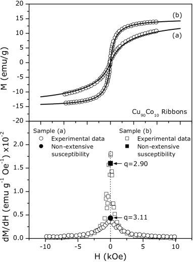
Figure 2: Top: Open circles are the experimental results, whereas the solid lines correspond to the average magnetization (Eq.2), considering a Log-Normal distribution (Eq.9). Bottom: dM/dH as a function of the applied magnetic field, where the magnetic susceptibility lies in the zero field limit. The predicted non-extensive magnetic susceptibility matches the experimental one, for both samples.

III.2 Distribution of critical temperatures

Campillo and co-workersCampillo et al. (2001) analyzed the magnetic properties of 200-nm thick films of La_0.67Ca_0.33MnO₃, which were grown under identical conditions onto five different single crystal substrates: MgO, Si, NdGaO₃, SrTiO₃, LaAlO₃. The films exhibit a strong substrate dependence of the magnetic properties, including, for instance, different values of Curie temperature $T_{C}$. On the other hand, the strain due to the growth mode induces inhomogeneities on the sampleCampillo et al. (2001); Ahn et al. (2004). Campillo verified that these inhomogeneities depend on the substrate character and therefore they determined the $T_{C}$ distribution for each thick film.

The authors considered that the magnetization of a small and homogeneous region is given by:

$$\mathcal{M}(m_{0},T_{C},T,\beta)=m_{0}\left(1-\frac{T}{T_{C}}\right)^{\beta}\theta(T_{C}-T)$$ (11)

where $\theta(x)$ is the Heavyside Step function. Supposing a Normal distribution of Curie temperatures

$$f(T_{C})=\frac{1}{\sqrt{2\pi}\;\sigma}\;\exp\left(-\frac{\left(T_{C}-\langle T_{C}\rangle\right)^{2}}{2\;\sigma^{2}}\right)$$ (12)

where $\sigma$ is the standard deviation and $\langle T_{C}\rangle$ the first moment of the distribution, they could write the average magnetization:

$$\langle\mathcal{M}\rangle=\int_{0}^{\infty}\mathcal{M}(m_{0},T_{C},T,\beta)\;f(T_{C})dT_{C}$$ (13)

and fit the corresponding $M$ vs. $T$ curves, for all samples available. From those fits, the authors could obtain a linear relationship between the standard deviation $\sigma$ and the mean value $\langle T_{C}\rangle$ of the samples analyzed; $\langle T_{C}\rangle=272-1.6\;\sigma$, as presented in figure 3(a).

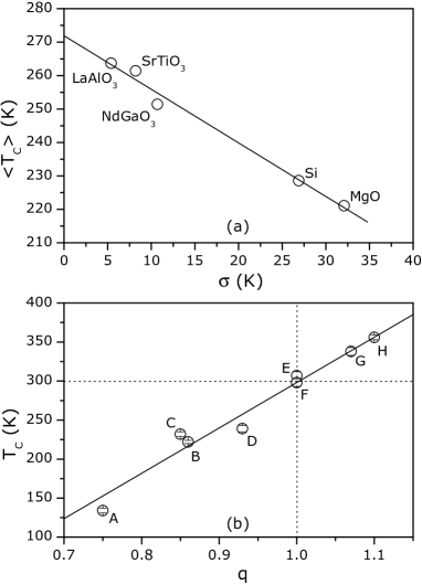
Figure 3: (a) First moment $\langle T_{C}\rangle$ of the Curie temperature distribution as a function of the standard deviation $\sigma$, obtained fitting the $M$ vs. $T$ curves of La_0.67Ca_0.33MnO₃ manganites deposited onto five different single crystal substrates: MgO, Si, NdGaO₃, SrTiO₃, LaAlO₃. After Campillo et al. Campillo et al. (2001). (b) Curie temperature as a function of the $q$ parameter, obtained from the fit, using the generalized Brillouin functionReis et al. (2002b, a), of the $M$ vs. $T$ curves of those manganites referred in Table 1.

On the other hand, in our previous workReis et al. (2002a), we used the Generalized Brillouin functionReis et al. (2002b, a), a non-extensive magnetic equation of state, to fit the $M$ vs. $T$ curves obtained from those manganites presented in Table 1. From that study emerges a linear relationship between $T_{C}$, a quantity intrinsic to the material, and the $q$ parameter, a quantity intrinsic to the non-extensive statistics; $T_{C}=-283+581\;q$, as presented in figure 3(b).

Table 1: Manganites, and the respective references, in which its $M$ vs. $T$ curves were analyzed using the generalized Brillouin functionReis et al. (2002b, a) in order to obtain the corresponding $q$ parameter. The Label column corresponds to the figure 3(b). The choice of compounds was made such as to cover a wide range of $T_{c}$ values within the ferromagnetic phase, but it was random in any other aspect.

Label	Compound	Ref.
A	La0.62Y0.07Ca0.31MnO3+δ	McGuire et al. (1998)
B	La0.875Sr0.125MnO3+δ	Mitchell et al. (1996)
C	La0.5Ca0.5MnO3	Levy et al. (2000)
D	La0.83Sr0.17Mn0.98Fe0.02O3	Tkachuk et al. (1998)
E	La0.89Sr0.11MnO3+δ	Reis et al. (2002a)
F	La0.75Ba0.25MnO3	Ju et al. (2000)
G	La0.5Ba0.5MnO3	Ju et al. (2000)
H	La0.7Sr0.3Mn0.9Ru0.1O3	Ranjan and Manoharan (2000)

Comparing the results obtained by our ownReis et al. (2002a) (figure 3(b)) and CampilloCampillo et al. (2001) (figure 3(a)), we could estimate a relation between the standard deviation $\sigma$ and the $q$ parameter:

$$\sigma\propto(1-q)$$ (14)

reinforcing the idea that the $q$ parameter is related to the inhomogeneities of the system. Note that, $q\rightarrow$1 imply in $\sigma\rightarrow$0, i.e., the extensive (Maxwell-Boltzmann) limit corresponds to the homogeneous case.

IV Concluding remarks

Summarizing, in the present work we shown that the $q$ parameter measures the inhomogeneity and dynamics of a given inhomogeneous magnetic system. We stress that the measured $q$, obtained from scanning tunnelling spectroscopy on manganites (a microscopic information), is able to predict a thermodynamic quantity, the bulk magnetization (a macroscopic information); the entropic parameter contains the dynamics, connecting the microscopic and macroscopic worlds. Thus, the present work shows a clear combination of dynamics and statistics, the key role to describe complex systems. The present model was also successful applied to a series of La_0.67Ca_0.33MnO₃ thick filmsCampillo et al. (2001) and melt-spun Cu₉₀Co₁₀ ribbonsFerrari et al. (1997); and the results reinforce the conclusions made in this work.

V Acknowledgements

We acknowledge CAPES-Brasil and GRICES-Portugal. MSR acknowledges the FCT Grant No. BPD/23184/2005. We are also thankful to P.B. Tavares and A.M.L. Lopes (sample preparation), and M.P. Albuquerque and A.R. Gesualdi (some discussion on image processing).

References

- (1) For a complete and updated list of references, see the web site: tsallis.cat.cbpf.br/biblio.htm.
- Tsallis (2001) C. Tsallis, Nonextensive Statistical Mechanics and Its Applications (Springer-Verlag, Heidelberg, 2001), chap. Nonextensive Statistical Mechanics and Thermodynamics: Historical Background and Present Status, eds. S. Abe and Y. Okamoto.
- Lorenzana et al. (2001a) J. Lorenzana, C. Castellani, and C. D. Castro, Phys. Rev. B 64, 235127 (2001a).
- Lorenzana et al. (2001b) J. Lorenzana, C. Castellani, and C. D. Castro, Phys. Rev. B 64, 235128 (2001b).
- Moreo et al. (1999) A. Moreo, S. Yunoki, and E. Dagotto, Science 283, 2034 (1999).
- Dagotto et al. (2001) E. Dagotto, T. Hotta, and A. Moreo, Phys. Rep. 344, 1 (2001).
- Ausloos et al. (2002) M. Ausloos, L. Hubert, S. Dorbolo, A. Gilabert, and R. Cloots, Phys. Rev. B 66, 174436 (2002).
- Dagotto (2003) E. Dagotto, Nanoscale phase separation and colossal magnetoresistance: The physics of manganites and related compounds. (Springer-Verlag, Heidelberg, 2003).
- Becker et al. (2002) T. Becker, C. Streng, Y. Luo, V. Moshnyaga, B. Damaschke, N. Shannon, and K. Samwer, Phys. Rev. Lett. 89, 237203 (2002).
- Kumar and Majumdar (2004) S. Kumar and P. Majumdar, Phys. Rev. Lett. 92, 126602 (2004).
- Ahn et al. (2004) K. H. Ahn, T. Lookman, and A. R. Bishop, Nature 428, 401 (2004).
- Reis et al. (2002a) M. S. Reis, J. C. C. Freitas, M. T. D. Orlando, E. K. Lenzi, and I. S. Oliveira, Europhys. Lett. 58, 42 (2002a).
- Reis et al. (2002b) M. S. Reis, J. P. Araújo, V. S. Amaral, E. K. Lenzi, and I. S. Oliveira, Phys. Rev. B 66, 134417 (2002b).
- Reis et al. (2003) M. S. Reis, V. S. Amaral, J. P. Araújo, and I. S. Oliveira, Phys. Rev. B 68, 014404 (2003).
- Guimar es (1998) A. P. Guimar es, Magnetism and Magnetic Resonance in Solids (John Wiley, New York, 1998).
- (16) In our previous workReis et al. (2003), we derived the two-branched Generalized Langevin Function. However, further calculations lead us to a more concise and general expression, valid for any real value of and (Eq.3).
- Beck (2001) C. Beck, Phys. Rev. Lett. 87, 180601 (2001).
- Beck and Cohen (2003) C. Beck and E. G. D. Cohen, Physica A 322, 267 (2003).
- Renner et al. (2002) C. Renner, G. Aeppli, B. Kim, Y. Soh, and S. Cheong, Nature 416, 518 (2002).
- Fath et al. (1999) M. Fath, S. Freisem, A. A. Menovsky, Y. Tomioka, J. Aarts, and J. A. Mydosh, Science 285, 1540 (1999).
- Lu et al. (1997) Q. Lu, C. Chen, and A. deLozanne, Science 276, 2006 (1997).
- Zhang et al. (2002) L. Zhang, C. Israel, A. Biswas, R. L. Greene, and A. deLozanne, Science 298, 805 (2002).
- Ferrari et al. (1997) E. Ferrari, F. Silva, and M. Knobel, Phys. Rev. B 56, 6086 (1997).
- Murillo et al. (2004) N. Murillo, H. Grande, I. Etxeberria, J. DelVal, J. Gonzalez, S. Arana, and F. Gracia, Journal of Nanoscience and Nanotechnology 4, 1056 (2004).
- Panissod et al. (2001) P. Panissod, M. Malinowska, E. Jedryka, M. Wojcik, S. Nadolski, M. Knobel, and J. Schmidt, Phys. Rev. B 63, 014408 (2001).
- Campillo et al. (2001) G. Campillo, A. Berger, J. Osorio, J. Pearson, S. Bader, E. Baca, and P. Prieto, J. Magn. Magn. Mater. 237, 61 (2001).
- McGuire et al. (1998) T. R. McGuire, P. R. Duncombe, G. Q. Gong, A. Gupta, X. W. Li, S. J. Pickart, and M. L. Crow, J. Appl. Phys. 83, 7076 (1998).
- Mitchell et al. (1996) J. F. Mitchell, D. N. Argyriou, C. D. Potter, D. G. Hinks, J. D. Jorgensen, and S. D. Bader, Phys. Rev. B 54, 6172 (1996).
- Levy et al. (2000) P. Levy, F. Parisi, G. Polla, D. Vega, G. Leyva, H. Lanza, R. S. Freitas, and L. Ghivelder, Phys. Rev. B 62, 6437 (2000).
- Tkachuk et al. (1998) A. Tkachuk, K. Rogackia, D. E. Brown, B. Dabrowski, A. J. Fedro, C. W. Kimball, B. Pyles, X. Xiong, D. Rosenmann, and B. D. Dunlap, Phys. Rev. B 57, 8509 (1998).
- Ju et al. (2000) H. L. Ju, Y. S. Nam, J. E. Lee, and H. S. Shin, J. Magn. Magn. Mater. 219, 1 (2000).
- Ranjan and Manoharan (2000) K. S. Ranjan and S. S. Manoharan, Appl. Phys. Lett. 77, 2382 (2000).