Spin Correlations and Finite-Size Effects in the One-dimensional Kondo Box

Abstract

We analyze the Kondo effect of a magnetic impurity attached to an ultrasmall metallic wire using the density matrix renormalization group. The spatial spin correlation function and the impurity spectral density are computed for system sizes of up to $L=511$ sites, covering the crossover from $L<\ell_{K}$ to $L>\ell_{K}$, with $\ell_{K}$ the spin screening length. We establish a proportionality between the weight of the Kondo resonance and $\ell_{K}$ as function of $L$. This suggests a spectroscopic way of detecting the Kondo cloud.

Scanning tunneling techniques have recently allowed to observe the Kondo effect of a magnetic atom in an ultrasmall metallic box odom00 , possibly providing a direct probe of the long sought-after Kondo screening cloud. The Kondo effect is characterized by a narrow resonance of width $\sim T_{K}$, the Kondo temperature, at the Fermi energy $\varepsilon_{F}$ hewson93 . It is intimately related to the formation of a many-body singlet state, comprised of the impurity spin and a cloud of surrounding, spin-correlated electrons, the so-called Kondo spin screening cloud. Its spatial extent is vital for the coupling between neighboring Kondo impurities in a metal and, hence, is at the heart of spatial magnetic correlations and ordering transitions in Kondo and Anderson lattices and also in Hubbard or $t-J$ systems, which exhibit local Kondo physics, as has been demonstrated by the dynamical mean field theory (DMFT) treatment of the problem georges96 . However, while the spectral and thermodynamic features of Kondo impurities have been well understood hewson93 , the structure of the Kondo cloud has remained controversial for a long time. Researchers have been looking intensively for ways of observing the Kondo cloud. These include the Knight shift slichter74 and recently theoretical investigations of the persistent current affleck01 or the conductance affleck02 in mesoscopic Kondo systems. For about 25 years it was generally believed, and in the 1990s supported by scaling arguments affleck96 , that the Kondo cloud is characterized by a single length scale, $\xi_{K}=\hbar v_{F}/T_{K}$. It is the spin coherence length, i.e. the distance traveled by a scattered electron with Fermi velocity $v_{F}$, until the impurity spin (whose lifetime is $\hbar/T_{K}$) flips. Although $\xi_{K}$ can reach almost macroscopic values ($\xi_{K}\approx 10^{3}k_{F}^{-1}$ for $T_{K}=1\ K$, $k_{F}$ being the Fermi wave number), it has never been observed in experiments.
Only recently it was realized that another length scale, $\ell_{K}$, arises in a $d$-dimensional Kondo system, if all conduction electron states couple equally to the impurity spin thimm99 . It is the length of a finite-size conduction electron sea, the “Kondo box”, which is so small that its level spacing $\Delta$ is comparable to $T_{K}$ of the bulk system and cuts off the logarithmic Kondo correlations. Therefore, a box of length $\ell_{K}$ sustains just one conduction electron state within the Kondo scale $T_{K}$ to form the Kondo singlet affleck00 , i.e. $\ell_{K}$ is the size of the Kondo cloud, the Kondo screening length. Equating $\Delta=T_{K}$, with $\Delta$ the inverse of the typical density of states (DOS) in a box of size $\ell_{K}$, $N(\ell_{K})=(\ell_{K}/2\pi)^{d}S_{d}k_{F}^{d-1}/(\hbar v_{F})$, yields,

$$\ell_{K}=2\pi\left(\xi_{K}/S_{d}k_{F}^{d-1}\right)^{1/d}\ ,$$ (1)

with $S_{d}$ the surface of the $d$-dimensional unit sphere thimm99 . Hence, $\ell_{K}$ is an intermediate length scale, which for $d\geq 2$ can be substantially smaller than the coherence length, $1/k_{F}<\ell_{K}<\xi_{K}$, and $\ell_{K}\approx\xi_{K}$ only in effectively 1D systems. Another length scale, $\ell_{RKKY}$, would arise in dilute Kondo systems as the one when the RKKY coupling between neighboring impurities equals $T_{K}$, $\ell_{RKKY}=[JN(k_{F}^{-1})]^{1/d}\ell_{K}<\ell_{K}$ affleck00 , where $JN(k_{F}^{-1})$ is the dimensionless spin coupling. The different physical meaning of $\xi_{K}$ and $\ell_{K}$ should be kept in mind for the design of related experiments. For example, experiments to detect the Kondo cloud via finite system size, like those proposed in Refs. affleck01 ; affleck02 , probe $\ell_{K}$ rather than $\xi_{K}$. These experiments should be performed on 1D wires in order for $\ell_{K}$ to be in an experimentally accessible range. 1D Kondo boxes have up to now been realized as ultrashort Carbon nanotubes odom00 , which, however, do not easily permit persistent affleck01 or transport affleck02 current measurements.

In this work we show numerical evidence that the Kondo cloud can be detected via spectroscopy of the Kondo resonance in a 1D Kondo box. To that end we establish a non-trivial proportionality between the Kondo spectral weight and the spin screening length as function of system size, using large-scale density matrix renormalization group (DMRG) calculations white92 ; kuehner99 . The systems considered here are 1D in the sense that the magnetic impurity is side-coupled to a finite chain of atoms only at a single site $x_{0}$ of the chain. This is different from the ultrasmall boxes considered in Refs. thimm99 ; schlottmann02 , where the effective hybridization was the same for all states in the box. The latter systems may have been realized most recently in molecules booth05 . As a result of the local coupling we observe strong mesoscopic variations of $T_{K}$ and of the spectral features. We analyze, under which mesoscopic conditions the above-mentioned proportionality prevails.

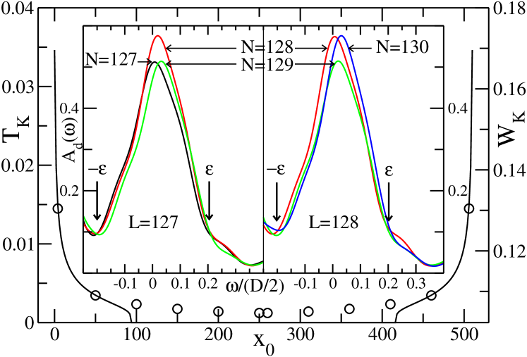
Figure 1: (Color online) Finite-size and even/odd effects in the 1D Kondo box. Solid line: $T_{K}$ as a function of impurity position $x_{0}$ for $L=511$, $N=512$, $V=0.35$ and open boundary conditions, as obtained from Eq. (3). Open circles: Weight of the Kondo peak, $W_{K}$, as defined in the text and in the inset. The results shown are for even $x_{0}$ only (see text). The inset shows the Kondo peak for $V=0.35$, $x_{0}=4$ and for various successive values of $L$ and $N$.

The Hamiltonian for an Anderson impurity with local energy $\varepsilon_{d}$ and on-site Coulomb repulsion $U$, side-coupled via the hybridization matrix element $V$ to the site $x_{0}$ on a 1D chain of $L$ sites, reads,

$$H = H_{ch}+\varepsilon_{d}\sum_{\sigma}d_{\sigma}^{\dagger}d_{\sigma}^{\phantom{\dagger}}+V\sum_{\sigma}\left[c_{x_{o}\sigma}^{\dagger}d_{\sigma}^{\phantom{\dagger}}+H.c.\right]$$ (2)

$$+ Ud_{\uparrow}^{\dagger}d_{\uparrow}^{\phantom{\dagger}}d_{\downarrow}^{\dagger}d_{\downarrow}^{\phantom{\dagger}}\ ,$$

where $H_{ch}=-t\sum_{\langle i,j\rangle,\sigma}c_{i\sigma}^{\dagger}c_{j\sigma}^{\phantom{\dagger}}$, $i,j=0,\dots,L-1$, is the free chain Hamiltonian with nearest-neighbor hopping $t>0$. For the evaluations we choose the total electron number $N$ near half bandfilling ($N=L\pm 2$, $\varepsilon_{F}\approx 0$) and use generic parameters for the model in the Kondo regime, $\varepsilon_{d}=-0.55$, $U=5$, and $V$ as indicated where appropriate. All energies are given in units of the half bandwidth $D=2t$. The Kondo spin coupling is given by $J=V^{2}[1/|\varepsilon_{d}|+1/(\varepsilon_{d}+U)]$.

$T_{K}$ in finite systems. As mentioned above, for this realistic model one expects large finite-size effects, because the effective impurity-chain coupling, which governs the low-energy Kondo physics, depends on the amplitudes of the free-electron eigenfunctions of the chain, $\Psi_{k}(x_{0})$, at the position $x_{0}$. The Kondo scale $T_{K}$ is defined as the temperature $T$ at which the 2nd order contribution to the spin scattering T-matrix equals the 1st order hewson93 , a condition which in the finite system reads,

$$-2J\sum_{k}\frac{|\Psi_{k}(x_{0})|^{2}}{\varepsilon_{k}-\varepsilon_{F}}\ \frac{1}{e^{-(\varepsilon_{k}-\varepsilon_{F})/T_{K}}+1}=1\ ,$$ (3)

with $\varepsilon_{k}$ the levels of the free chain. It is seen that $T_{K}$ itself depends on the impurity position $x_{0}$ affleck03 ; morr06 and on the system size $L$ as well. The strong $x_{0}$ dependence of $T_{K}(x_{0})$ shown in Fig. 1 is due to the increase of the 1D local DOS towards the ends of a chain with open boundary conditions zarand96 . If $x_{0}$ ist too close to the center of the chain (e.g. $|x_{0}/L-1/2|\lesssim 160$ in Fig. 1), the log contributions in Eq. (3) are cut off by the level spacing of the finite system before the breakdown of perturbation theory, so that the system stays in the perturbative regime for all temperatures, i.e. $T_{K}=0$ (Fig. 1). Hence, in an ultrasmall system the expressions for $\ell_{K}$ and $\xi_{K}$ discussed above can, at best, serve to obtain typical values for these quantities. We find that the width of the Kondo resonance for various $\varepsilon_{d}$, $U$, $V$ resembles roughly $T_{K}$ of Eq. (3), however obscured by the discreteness of the box spectrum. Detecting the Kondo cloud by varying the system size then becomes a nontrivial task, since $\ell_{K}$ itself depends on $L$. Detailed numerical calculations are, therefore, needed in order to incorporate these finite size effects and to extract the universal features that persist under these conditions.

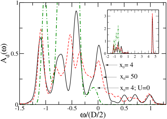
Figure 2: (Color online) The impurity spectral density $A_{d}(\omega)$ for $L=127$, $N=128$, $V=0.35$ and two different $x_{0}$; $\eta=0.05$. Comparison with the non-interacting spectrum ($U=0$) exhibits the Kondo enhancement of the peak near $\varepsilon_{F}=0$. The inset shows the upper Hubbard peak near $\omega=\varepsilon_{d}+U$.

Numerical method and testing. Applying an efficient DMRG code hand06 to the model Eq. (2), we have computed the (retarded) impurity Green’s function and the equal-time spin correlation function at $T=0$,

$$G_{d\sigma}(\omega) = \langle 0|\left[d_{\sigma}^{\phantom{\dagger}}\frac{1}{E+i\eta-H}d_{\sigma}^{\dagger}+d_{\sigma}^{\dagger}\frac{1}{E+i\eta-H}d_{\sigma}^{\phantom{\dagger}}\right]|0\rangle$$

$$K(r) = \langle 0|S^{z}_{i}S^{z}_{x}|0\rangle-\langle 0|S^{z}_{i}|0\rangle\langle 0|S^{z}_{x}|0\rangle\ ,$$ (5)

respectively, for system sizes of up to $L=511$. Here $\omega$ is the single-particle excitation energy relative to the many-body ground state energy $E_{0}$, $E=\omega+E_{0}$. $|0\rangle$ the DMRG many-body ground state and $S^{z}_{i}$, $S^{z}_{x}$ the z-components of the spin-1/2 operators on the impurity and on chain site $x$, $r=x-x_{0}$, respectively. The impurity spectral density is $A_{d\sigma}(\omega)=-\frac{1}{\pi}{\rm Im}G_{d\sigma}(\omega)$. Open boundary conditions are applied to facilitate convergence of the DMRG algorithm. They also appear appropriate for a wire (weakly) coupled to leads. For the dynamical quantities we have used both the correction vector (CV) method kuehner99 , and the Lanczos method (LM) hallberg95 . For the CV method, $m=200$ basis states were retained in each DMRG iteration, which proved sufficient to compute the residue of the CV $(\omega+i\eta-H)^{-1}d_{\sigma}^{\dagger}|0\rangle$ with a precision of $10^{-8}$ for each $\omega$. For the LM we used 3 to 5 target states, kept ($m=2600$) basis states and carried out 200 Lanczos steps to build the Krylov subspace. The comparison of the two methods for $L$ up to 128 yields excellent agreement (better than 0.1 per cent) for $\omega\lesssim T_{K}$ and still good agreement (better than 10 per cent) even for the highest $|\omega|\approx D$, where the LM becomes inaccurate. Scaling up the system size from $L=128$ to $L^{\prime}=511$ reduces the frequency range where Lanczos is accurate by a factor $L/L^{\prime}$, which was satisfactory for the calculations in the Kondo regime. For the largest systems ($L=511$) we, therefore, used the numerically less demanding LM.

Figure 3: (Color online) The average $C(r)$ of the spin correlation function $K(r)$ is shown as function of $1/r$ for $L=511$, $N=512$ and various hybridization strengths $V$; $r=x-x_{0}$, $x_{0}=4$. Inset: $K(r)$ showing RKKY oscillations. The $V=0.55$ curve is offset by -0.005 for clarity.

Note that all DMRG calculations are done in the canonical ensemble with fixed electron number $N$ and fixed total spin $S$, whereas experimental systems are usually coupled to a particle reservoir. Life-time effects of $N$ and $S$ are included as a Lorentzian (for the CV method) or Gaussian (for the LM) broadening $\eta$ of the energy levels, with $\eta=0.05$ below. $x_{0}$ is chosen near the end of the chain, where $T_{K}$ is large enough (see above and Fig. 1) so that we can sweep through the crossover from $\Delta>T_{K}$ to $\Delta<T_{K}$. Furthermore we choose $x_{0}$ to be even, because on all odd sites the chain wave function at $\varepsilon_{F}=0$ has a node, so that for small $L$ ($\Delta>T_{K}$) the impurity would be decoupled.

Results. The $T=0$ impurity spectrum $A_{d\sigma}(\omega)$ shown in Fig. 2 exhibits a rich multiple peak structure even in the single-particle spectral weight near $\omega\approx\varepsilon_{d}$, induced by the discrete local conduction electron spectrum even for the largest $L$, when the impurity is placed close to the boundary. The Kondo peak is identified in Fig. 2 as the one near $\omega=0$ through its systematically increasing weight as the interaction $U$ is switched on, as $L$ is increased (Fig. 4), or as $T_{K}$ is increased by moving the impurity from $x_{0}=50$ to $x_{0}=4$ (see also Fig. 1). The latter would correspond to decreasing $T$ thimm99 in a temperature dependent measurement. For the local impurity coupling $V$ in Eq. (2) we find that the particle number parity effect in the position of the spectral features (1 or 2 peaks within $|\omega|\lesssim T_{K}$) is essentially washed out by finite-size irregularities of the local conduction electron spectrum even for small level broadening $\eta$ (not shown), in contrast to the pronounced even/odd characteristics predicted for equal coupling to all conduction states thimm99 . However, the even/odd effect is seen in the inset of Fig. 1 as an enhancement of the Kondo peak for even as compared to odd $N$ for fixed system size $L$.

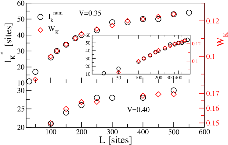
Figure 4: (Color online) The weight of the Kondo resonance $W_{K}$ and the numerically determined screening length $\ell_{K}^{*}$ as function of size $L$ for $x_{0}=4$ and $N=L+1$, $N$ odd.

The impurity-conduction electron spin correlation function $K(r)$, as computed from Eq. (5), is shown in the inset of Fig. 3. It displays RKKY oscillations with period $\lambda_{RKKY}=\pi/k_{F}=2a$ ($a=$lattice constant), Its overall weight yields $s^{-2}\sum_{r}K(r)=-n_{d}$, with $n_{d}$ the total impurity occupation number, confirming complete screening of the impurity spin, $s=1/2$. The average $C(r)=(K(r)+K(r+1))/2$ measures the spin content in the Kondo cloud at distance $r$, while $\Delta K(r)=|K(r)-K(r+1)|/2$ is the amplitude of the RKKY oscillations. $C(r)$ is shown in Fig. 3, together with the respective $\ell_{K}$ as calculated from Eqs. (1), (3). The expected $1/r^{d}$ behavior affleck96 is clearly seen for $1/k_{F}\ll r<\ell_{K}$ and $V=0.3,\ 0.34$. For smaller $\ell_{K}$ ($V=0.4$, $0.45$, $0.55$) the powerlaw range is too narrow to be observable. For $r\stackrel{{\scriptstyle>}}{{\sim}}\ell_{K}$, we find exponential decay, $C(r)\propto\exp(-2r/\ell_{K})$ (Fig. 3), and similar for $\Delta K(r)$. This is expected for the correlator of two non-conserved quantities, like $S_{i}^{z}$, $S_{x}^{z}$, with a finite correlation length. In the asymptotic region, $r\gg\ell_{K}$, the exponential behavior should be overidden by the slower powerlaw decay, $C(r)\propto 1/r^{d+1}$, expected from general Fermi liquid arguments ishii78 ; affleck98 . The numerical data show indications of this crossover for the largest $L$ and the smallest $\ell_{K}$. A more detailed analysis of the complex $r$-dependence will be presented elsewhere.

Figure 5: (Color online) $W_{K}$ like in Fig. 4, but for $N$ even.

For $V=0.3$ the $\ell_{K}$ from Eq. (1) is $936>L$. $C(r)$ is then not cut off by $\ell_{K}$ but by $L$, and the conduction electron spin density necessary for complete spin screening is accumulated at shorter distances, leading to a positive $y$-axis intersection, see Fig. 3. This displays the difficulty in extracting $\ell_{K}$ directly from finite systems and the limited applicability of Eqs. (1), (3) for this purpose. Therefore, we combine the results for $A_{d\sigma}(\omega)$ and $C(r)$ to obtain an experimental signature of the (bulk) screening length $\ell_{K}$ in the finite-size spectra. In doing so one must observe that for $L\lesssim\ell_{K}$, $\ell_{K}$ itself becomes size and position dependent according to Eqs. (1), (3) and that for our system with fixed total spin there is always a total spin $1/2$ in the cloud, no matter how small $L$. Therefore, we define the screening length of the finite system, $\ell_{K}^{*}(L)$, by the volume needed to host a certain fraction $c$ of the total spin, $s^{-2}\int_{0}^{\ell_{K}^{*}}drK(r)=c$, where $s=1/2$ is the electron spin. The Kondo spectral weight is defined as $W_{K}(L)=\int_{-\varepsilon^{\prime}}^{\varepsilon}d\omega A_{d\sigma}(\omega)$ (c.f. Fig. 1, inset), where the boundaries $-\varepsilon^{\prime}$, $\varepsilon$, are chosen so as to cover the Kondo resonance, identified numerically as that part of the spectrum around $\varepsilon_{F}$ which increases as $U$ is switched on (c.f. Fig. 2). The results for both quantities are shown in Figs. 4, 5 for $c=0.75$ and $\varepsilon=\varepsilon^{\prime}=0.2$. For odd particle number $N$ (Fig. 4) the nontrivial proportionality $\ell_{K}^{*}(L)/W_{K}(L)=\alpha(J)$ for the complete range of $L$ is established. We checked that it persists independent of the precise choice of $\varepsilon$, $\varepsilon^{\prime}$ and $c$. Both $W_{K}(L)$ and $\ell_{K}^{*}(L)$ are logarithmically suppressed with decreasing $L$ (inset of Fig. 4). For universality reasons we expect the proportionality to extend out to $L\to\infty$, where $\ell_{K}^{*}(L)\to\ell_{K}(\infty)$ must saturate at its bulk value. The proportionality $W_{K}(L)\propto\ell_{K}^{*}(L)$ persists for different values of $J$ (Fig. 4), and the corresponding $\ell_{K}^{*}(L)$ can be scaled on top of each other by plotting $\ell_{K}^{*}(L)/\ell_{K}^{*}(J)$ vs $L/\ell_{K}^{*}(J)$, with the scaling parameter $\ell_{K}^{*}(J)\approx\ell_{K}(\infty)$. The above relation can be used to determine $\ell_{K}^{*}(L)$ by a spectroscopic measurement and to extrapolate to its bulk value, once the proportionality constant $\alpha(J)$ is determined. Fig. 5 displays $\ell_{K}^{*}$ for even $N$, showing an earlier saturation compared to Fig. 4, as expected from the even/odd effect thimm99 . However, we find $W_{K}(L)\approx const.$ in this case, breaking the above proportionality. By an analysis of the spectra this is traced back to the fact that for the parameters of Fig. 5 the impurity spectrum is dominated by a strong $L$-independent single-particle peak inherited from the free conduction band, while the spin structure, $C(r)$, retains its $L$-dependence. This is to emphasize that it is essential to identify the $\varepsilon_{F}$ peak as a Kondo peak first, e.g. by its logarithmic $T$ or $L$ dependence, before the above analysis can be applied.

To conclude, we have analyzed the spectral and the spin structure of ultrasmall Kondo systems in the presence of strong finite-size fluctuations and even/odd effects using DMRG. Despite these non-universal effects we have identified a procedure to measure the spin screening length $\ell_{K}$ by tunneling spectroscopy, e.g. on carbon nanotube Kondo boxes. Further research is needed to understand the relation $\ell_{K}^{*}(L)=\alpha W_{K}(L)$ and to determine the proportionality factor $\alpha(J)$.

We acknowledge useful discussions with I. Affleck and S. White. This work was supported in part by DFG through grants KR1726/1, SFB 608, and SP1073.

Electronic address: kroha@physik.uni-bonn.de

References

- (1) T. W. Odom et al., Science 290, 1549 (2000).
- (2) For a comprehensive overview see A. C. Hewson, The Kondo Problem to Heavy Fermions, CUP (1993).
- (3) A. Georges et al., Rev. Mod. Phys. 68, 13 (1996).
- (4) J. P. Boyce and C. P. Slichter, Phys. Rev. Lett. 32, 61 (1974); Phys. Rev. B 13, 379 (1976).
- (5) I. Affleck and P. Simon, Phys. Rev. Lett. 86, 2854 (2001); 88, 139701 (2002); H. P. Eckle, H. Johannesson, and C. A. Stafford, Phys. Rev. Lett. 87, 016602 (2001); 88, 139702 (2002); P. Simon and I. Affleck, Phys. Rev. B 64, 085308 (2001); E. S. S/orensen and I. Affleck, Phys. Rev. Lett. 94 086601 (2005).
- (6) P. Simon, I. Affleck, Phys. Rev. Lett. 89, 206602 (2002);
- (7) E. S. S/orensen and I. Affleck, Phys. Rev. B 53 9153 (1996); V. Barzykin and I. Affleck, Phys. Rev. Lett. 76, 4959 (1996);
- (8) W. B. Thimm, J. Kroha, and J. v. Delft, Phys. Rev. Lett. 82, 2143 (1999).
- (9) V. Barzykin and I. Affleck, Phys. Rev. B 61 6170 (2000).
- (10) P. Simon and I. Affleck, Phys. Rev. B 68, 115304 (2003).
- (11) E. Rossi and D. K. Morr, cond-mat/0602002.
- (12) G. Zaránd and L. Udvardi, Phys. Rev. B 54, 7606 (1996).
- (13) S. R. White, Phys. Rev. Lett. 69, 2863 (1992); Phys. Rev. B 48, 10345 (1993).
- (14) P. Schlottmann, Phys. Rev. B 65, 024420 (2002); Acta Phys. Pol. B 34, 1351 (2003).
- (15) C. H. Booth et al., Phys. Rev. Lett. 95, 267202 (2005).
- (16) T. Hand, PhD Thesis, Universität Bonn (2006).
- (17) T. Kühner and S. R. White, Phys. Rev. B 60, 335 (1999).
- (18) K. Hallberg, Phys. Rev. B 52, R9827 (1995).
- (19) H. Ishii, J. Low Temp. Phys. 32, 457 (1978).
- (20) V. Barzkin and I. Affleck, Phys. Rev. B 57, 432 (1998).