Determination of the interactions in confined macroscopic Wigner islands: theory and experiments

Abstract

Macroscopic Wigner islands present an interesting complementary approach to explore the properties of two-dimensional confined particles systems. In this work, we characterize theoretically and experimentally the interaction between their basic components, viz., conducting spheres lying on the bottom electrode of a plane condenser. We show that the interaction energy can be approximately described by a decaying exponential as well as by a modified Bessel function of the second kind. In particular, this implies that the interactions in this system, whose characteristics are easily controllable, are the same as those between vortices in type-II superconductors.

1 Introduction

The recent development of in-situ imaging techniques has allowed new experimental investigations of two-dimensional mesoscopic devices consisting in small numbers of interacting confined particles. For instance, in type-II superconductors, SQUID microscopy hata03 or the multiple-small-tunnel junction method kanda04 have made possible the tracking of the vortices. Even more recently, stable and metastable vortex configurations in superconducting disks were observed using a Bitter decoration technique grigorieva06 . Many other systems are governed by the same physics: an interparticle interaction, a confining potential, and possibly a thermal activation overview .

In parallel with the experiments, the simplicity of the input ingredients has allowed the development of numerical simulations to determine both the equilibrium configurations and the dynamics of these systems. However, when the energy levels are very close, the uncertainties inherent in the numerical simulations make the confrontation with the experiments necessary.

The difficulties in controlling exhaustive sets of experimental parameters in real mesoscopic systems, such as the pinning or the interaction strengths, have led us to devise an analogue macroscopic experimental set-up, consisting in macroscopic Wigner islands, whose characteristics are easily tunable. As illustrated in Fig. 1, our macroscopic Wigner islands are constituted by millimetric stainless steel spheres (of radius $R=0.4$ mm and mass $m=2.15\,\mathrm{mg}$), sitting inside a horizontal plane condenser of height $h=1.5\,\mathrm{mm}$. The bottom electrode of the condenser is a doped silicon wafer, whereas the top one is a transparent conducting glass, thus allowing a direct capture of the position of the spheres by means of a camera placed above the experimental device. A metallic frame of height $h_{c}=1.5\,\mathrm{mm}$, intercalated between the two electrodes and in electric contact with the bottom one, confines the spheres. Note that the confining frame could be set to a different potential than the bottom electrode, but, for simplicity, in the following we will focus on the equality case. When a potential difference $V_{0}$ is applied to the condenser, the spheres become charged, repel each other and spread throughout the whole available space, electrostatically confined by the outside frame. The voltage $V_{0}$ goes typically from a few hundred Volts to a thousand, above which the condenser breaks down. By mechanically shaking the whole system, we can thermalize it: the spheres acquire a brownian motion brownian and obey Boltzmann statistics, in which the shaking amplitude plays the role of an effective temperature coupier05 .

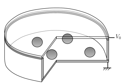
Figure 1: Section of the experimental device. Here the frame is circular, as it will be used in section 4.

We then have a system in which the interaction between the spheres, as well as the confining potential, can be easily adjusted. This device has been previously used to study small confined systems stjean01 ; stjean02 ; in such systems, as it has been shown in numerous numerical studies campbell79 ; bedanov94 ; lai99 , the equilibrium positions and the dynamics are highly dependent upon the interaction between the particles. The same experimental set-up can be used to study pinning problems in two-dimensional elastic lattices. Indeed, defect-free lattices of a few thousand spheres can be obtained stjean04 . Again, the behavior of the system, in particular far from the equilibrium, highly depends on the interaction potential.

The comparison of our experimental equilibrium positions with the calculated ones, for up to thirty particles confined by a potential with axial symmetry, had led us to think that our interparticle interaction potential was logarithmic, at least within the experimental distance range stjean01 . The equilibrium configurations were also determined with an elliptic confinement stjean02 : the ground state configuration for 17 particles has been compared with the one for 17 vortices resulting from the minimization of the Ginzburg-Landau free energy in a mesoscopic type-II superconductor of the same geometry meyers00 . It has been suggested to the authors of the numerical study that the configuration that they presented was not the fundamental state but the first excited level, as they finally confirmed private . Let us remind that the intervortices interaction is described by the modified Bessel function of the second kind $K_{0}$ degennes , which has the following asymptotic behaviors:

$$K_{0}(r/\lambda) {\sim}\atop{r\to 0} -\ln(r/\lambda)$$ (1)

$${\sim}\atop{r\to\infty} \sqrt{\frac{\pi\lambda}{2r}}e^{-r/\lambda}.$$ (2)

All these indications on the nature of the interparticle interaction are indirect evidences and depend on already existing and studied interactions. Thus, they need to be confirmed and quantified.

In this paper, we calculate numerically this interaction by considering the electrostatic problem of two spheres in electric contact with one of the electrode of an infinite plane condenser. Section 2 is dedicated to the numerical resolution of the problem. First, the Laplace equation is formally solved by means of a multipolar expansion. The numerically obtained electrostatic potential allows to calculate the electrostatic energy of the system, from which the interaction energy between two spheres is derived. In the range of distances in which the numerical calculations can be made with sufficient accuracy, the interaction energy is well fitted by a decaying exponential as well as by a modified Bessel function $K_{0}$, both being controlled only by two parameters: their amplitude and their screening length. In section 3, we determine a simple approximation of the confining potential in the case of a circular frame, by considering the frame as a hedge of spheres over which the intersphere interaction energy can be integrated. A correction of the amplitude of the confining potential must be introduced to take into account the height difference between the interacting spheres and the frame. This is done in section 4, where the equilibrium configurations for up to 30 spheres and a circular frame are calculated. Comparisons with the experimental data allow to adjust the amplitude of the confinement and to validate the model.

2 Interaction between two spheres

2.1 Determination of the electrostatic potential

We consider an infinite planar parallel plates condenser of thickness $h$; its lower plate is kept at zero potential and its upper plate is kept at the fixed potential $V_{0}$. On the lower plate, in electric contact with it, sit two conducting spheres of radius $R<h/2$; the centers of the two spheres are separated by the distance $d\geq 2R$. We introduce a Cartesian coordinate system $\mathbf{r}=(x,y,z)$ having the $z$-axis orthogonal to the plates of the condenser, with $z=0$ (resp. $z=h$) on the lower (resp. upper) plate; we choose the $x$ and $y$-axis such that the centers of the two spheres are situated at $x=\pm d/2$ and $y=0$. Furthermore, we introduce two local Cartesian coordinate systems $\mathbf{r}_{-}=(x_{-},y_{-},z_{-})$ and $\mathbf{r}_{+}=(x_{+},y_{+},z_{+})$, centered, respectively, on the left and right sphere (see Fig. 2), and their corresponding spherical systems of coordinates $(r_{-},\theta_{-},\phi_{-})$ and $(r_{+},\theta_{+},\phi_{+})$:

$$x_{\pm} = x\mp d/2=r_{\pm}\sin\theta_{\pm}\cos\phi_{\pm},$$ (3)

$$y_{\pm} = y=r_{\pm}\sin\theta_{\pm}\sin\phi_{\pm},$$ (4)

$$z_{\pm} = z-R=r_{\pm}\cos\theta_{\pm}.$$ (5)

To determine the interaction between the conducting spheres, we must solve the Laplace equation

$$\nabla^{2}V=0,$$ (6)

for the electric potential $V(\mathbf{r})$, with the boundary conditions that $V=0$ on the lower plate and on the surface of the spheres, and $V=V_{0}$ on the upper plate. To this aim, we begin to write the total electric potential $V(\mathbf{r})$ as the sum of the potential $V_{0}\,z/h$ of the empty condenser plus a perturbation due to the presence of the two spheres

$$V(\mathbf{r})=V_{0}\left[\frac{z}{h}+v(\mathbf{r})\right].$$ (7)

The normalized perturbation $v(\mathbf{r})$ is the solution of the Laplace equation (6) that is regular in the space inside the condenser and outside the spheres, and that satisfies the boundary conditions

$$v(x,y,z=0) = v(x,y,z=h)=0,$$ (8)

$$v(r_{-}=R,\theta_{-},\phi_{-}) = -\frac{z(r_{-}=R,\theta_{-})}{h},$$ (9)

$$v(r_{+}=R,\theta_{+},\phi_{+}) = -\frac{z(r_{+}=R,\theta_{+})}{h},$$ (10)

$$v(|\mathbf{r}|\to\infty) = 0,$$ (11)

where $z(r_{-}=R,\theta_{-})$ [resp. $z(r_{+}=R,\theta_{+})$] is the $z$-coordinate of the point on the left (resp. right) sphere of local spherical coordinates $(r_{-}=R,\theta_{-},\phi_{-})$ [resp. $(r_{+}=R,\theta_{+},\phi_{+})$]; explicitly

$$z(r_{\pm}=R,\theta_{\pm})=R(1+\cos\theta_{\pm}).$$ (12)

Figure 2: Geometry for the electrostatic interaction of two spheres inside a parallel plates condenser.

To determine the perturbation $v(\mathbf{r})$, we start by considering the solutions $g_{\ell m}(\mathbf{r})$ of the Laplace equation (6), regular at infinity, obtained by separation of variables in the spherical coordinates $(r_{-},\theta_{-},\phi_{-})$:

$$g_{\ell m}(\mathbf{r})=\frac{{P_{\ell}}^{m}(\cos\theta_{-})h^{\ell+1}}{r_{-}^{\ell+1}}\cos(m\phi_{-}),$$ (13)

where the ${P_{\ell}}^{m}(\cos\theta_{-})$, with $\ell=0,1,2,\ldots$ and $0\leq m\leq\ell$, are the associated Legendre functions of the first kind abramowitz :

$${P_{\ell}}^{m}(t)=\frac{(-1)^{\ell+m}}{2^{\ell}\,\ell!}\left(1-t^{2}\right)^{m/2}\frac{d^{\ell+m}}{dt^{\ell+m}}\left(1-t^{2}\right)^{\ell}.$$ (14)

The elementary solutions (13) correspond to the usual terms of the expansion of the electrostatic potential in multipolar moments landau ; they are singular only at the center of the left sphere, $r_{-}=0$. The factors $h^{\ell+1}$ in their definition have been introduced to make them dimensionless. Note also that we retained only the harmonics $\cos(m\phi_{-})$, that satisfy the symmetry with respect to the $(x,z)$-plane of the present geometry. To construct, starting from the multipoles (13), a suitable complete basis of harmonic functions for our situation, we make a set of infinite mirror images of the potentials (13) through the two plates of the condenser $z=0$ and $z=h$, such that the boundary conditions (8) are automatically satisfied, and we symmetrize the resulting potential through the $(y,z)$-plane, as required by our geometry. The resulting base functions are therefore

$$G_{\ell m}(\mathbf{r})=\sum_{k=-\infty}^{\infty}\Big{[}g_{\ell m}(x,y,z+2kh)$$

$$-g_{\ell m}(x,y,-z+2kh)+g_{\ell m}(-x,y,z+2kh)$$

$$-g_{\ell m}(-x,y,-z+2kh)\Big{]};$$ (15)

they are regular in the volume inside the condenser and outside the spheres, since their only singularities are at the centers of the spheres and at their successive mirror images through the two plates of the condenser, i.e., at $(x=\pm d/2,y=0,z=\pm R+2kh)$, with $k=0,\pm 1,\pm 2,\ldots$. Using this set of base functions, we decompose the perturbation $v(\mathbf{r})$ as

$$v(\mathbf{r})=\sum_{\ell=0}^{\infty}\sum_{m=0}^{\ell}v_{\ell m}G_{\ell m}(\mathbf{r}).$$ (16)

The unknown coefficients $v_{\ell m}$ depend on the distance $d$ between the two spheres and can be determined by imposing the remaining boundary conditions (9) and (10) on the two spheres. Since the basis functions (2.1) are symmetric with respect to the $(y,z)$-plane, only one of the two conditions has to be imposed. This is most efficiently done by projecting the boundary condition (9) on the set of functions ${P_{\ell^{\prime}}}^{m^{\prime}}(\cos\theta_{-})\cos(m^{\prime}\phi_{-})$, that represents a complete set of orthogonal functions—with the required symmetry with respect to the $(x,z)$ plane—on the left sphere. The resulting boundary equations are therefore

$$\sum_{\ell=0}^{\infty}\sum_{m=0}^{\ell}v_{\ell m}\!\! \int_{0}^{\pi}\!\!\!\sin\theta_{-}d\theta_{-}\!\int_{0}^{2\pi}\!\!\!d\phi_{-}\Big{[}G_{\ell m}(r_{-}\!=\!R,\theta_{-},\phi_{-})\times$$ (17)

$${P_{\ell^{\prime}}}^{m^{\prime}}(\cos\theta_{-})\cos(m^{\prime}\phi_{-})\Big{]}=$$

$$\left\{\matrix{-\displaystyle\frac{4\pi R}{h}&\mbox{if $\ell^{\prime}=m^{\prime}=0$}\hfill\cr&\cr-\displaystyle\frac{4\pi R}{3h}&\mbox{if $\ell^{\prime}=1$ and $m^{\prime}=0$}\hfill\cr&\cr 0&\mbox{otherwise}\hfill\cr}\right..$$

To numerically determine the coefficients $v_{\ell m}$, we truncate the sum in the left-hand side of Eq. (17) to a finite $\ell=\ell_{m}$, and we evaluate Eq. (17) for $m^{\prime}=0,1,\ldots,\ell^{\prime}$ and $\ell^{\prime}=0,1,\ldots,\ell_{m}$. This gives a set of $(\ell_{m}+1)(\ell_{m}+2)/2$ linear equations in the $(\ell_{m}+1)(\ell_{m}+2)/2$ unknowns $v_{\ell m}$. The integrals in Eq. (17), that determine the coefficients of this linear system, are computed numerically by truncating the mirror images sum in Eq. (2.1) to a finite $|k|=k_{m}$. By varying $\ell_{m}$ and $k_{m}$, we check for the convergence of the expansion.

2.2 Interaction energy

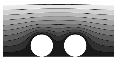
Figure 3: Contour plot of the electrostatic potential $V(\mathbf{r})$ in the plane $y=0$ for two spheres of radius $R=0.2\,h$ at the center to center distance $d=0.6\,h$. The spheres are indicated in white. Darker shadings correspond to lower values of $V(\mathbf{r})$.

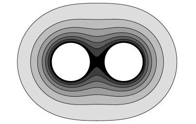
Figure 4: Same as figure 3 but in the plane $z=R$, i.e., the plane parallel to the plates of the condenser and passing through the centers of the spheres.

At fixed potential difference $V_{0}$, the mechanical interaction energy $F$ between the spheres is equal to the opposite of the electrostatic energy stored in the condenser

$$F=-\frac{1}{2}QV_{0},$$ (18)

where $Q$ is the charge stored on the upper plate $z=h$. The latter, for our infinite geometry, is actually infinite. However, its variation $\Delta Q$ due to the introduction of the spheres is finite: this is the charge associated to the potential perturbation $V_{0}\,v(\mathbf{r})$ in Eq. (7). To compute it, we make use of the reciprocity theorem, according to which, given two charge distributions $\rho(\mathbf{r})$ and $\rho^{\prime}(\mathbf{r})$ that create the potentials $V(\mathbf{r})$ and $V^{\prime}(\mathbf{r})$, respectively,

$$\int\rho(\mathbf{r})\,V^{\prime}(\mathbf{r})\,d\mathbf{r}=\int\rho^{\prime}(\mathbf{r})\,V(\mathbf{r})\,d\mathbf{r},$$ (19)

the volume integrals being performed over all the space durand . As $(\rho^{\prime},V^{\prime})$ system, we consider a plane parallel condenser having its lower plate $z=0$ at zero potential and upper plate $z=h$ at the potential $V_{0}$; its potential distribution is thus $V^{\prime}=V_{0}z/h$ for $0\leq z\leq h$, $V^{\prime}=0$ for $z\leq 0$ and $V^{\prime}=V_{0}$ for $z\geq h$. As $(\rho,V)$ system we consider the potential distribution having $V=V_{0}\,v(\mathbf{r})$ for $0\leq z\leq h$ and $V=0$ otherwise; its associated charge distribution has three contributions: a surface charge $\Delta\sigma_{-}(x,y)$ on the lower plate $z=0$, a surface charge $\Delta\sigma_{+}(x,y)$ on the upper plate $z=h$, and two point-like charge distributions centered on the two spheres, at $(x=\pm d/2,y=0,z=R)$, associated to the corresponding multipolar singularities of the perturbation $v(\mathbf{r})$. The surface integral of the charge distribution $\Delta\sigma_{+}(x,y)$ is equal to the charge variation $\Delta Q$ due to the introduction of the spheres inside the condenser:

$$\int_{z=h}\Delta\sigma_{+}(x,y)\,dx\,dy=\Delta Q.$$ (20)

Now:

$$\int\rho^{\prime}(\mathbf{r})\,V(\mathbf{r})\,d\mathbf{r}=0,$$ (21)

since $\rho^{\prime}$ is non-zero only for $z=0$ and $z=h$, where $V$ is zero. On the other hand,

$$\int\!\!\rho(\mathbf{r})\,V^{\prime}(\mathbf{r})\,d\mathbf{r}=V_{0}\int_{z=h}\!\!\!\!\Delta\sigma_{+}(x,y)\,dx\,dy+\frac{V_{0}}{h}\int_{\Omega_{R}}\!\!\rho(\mathbf{r})\,z\,d\mathbf{r}.$$ (22)

The last volume integral in this expression is performed in the region $\Omega_{R}$ made of two arbitrary volumes encircling the two centers of the spheres, where $\rho(\mathbf{r})$ is concentrated: it equals the $z$-component of the dipolar moment of the charge distribution $\rho(\mathbf{r})$ around the origin $\mathbf{r}=\mathbf{0}$. Using Poisson’s equation $\rho(\mathbf{r})=-\epsilon_{0}\nabla^{2}[V_{0}v(\mathbf{r})]$, where $\epsilon_{0}$ is the vacuum dielectric constant, by successive integrations by parts and application of the Green theorem, we obtain

$$\int_{\Omega_{R}}\!\!\rho(\mathbf{r})\,z\,d\mathbf{r}=\epsilon_{0}V_{0}\oint_{\partial\Omega_{R}}\left[v(\mathbf{r})\mathbf{z}\cdot\bm{\nu}-z\frac{\partial v}{\partial\nu}\right]\,dS,$$ (23)

where the surface integral is performed over two arbitrary surfaces $\partial\Omega_{R}$ of outward normal $\bm{\nu}$ around the two centers of the spheres and $\mathbf{z}$ is the unit normal in the $z$-direction. Taking for $\partial\Omega_{R}$ two spherical surfaces centered at $(x=\pm d/2,y=0,z=R)$ and using the decomposition (16), one obtains

$$\int_{\Omega_{R}}\!\!\rho(\mathbf{r})\,z\,d\mathbf{r}=8\pi\epsilon_{0}V_{0}h^{2}\left[v_{00}\frac{R}{h}+v_{10}\right].$$ (24)

In fact, the only terms in the multipoles (13) having a non-zero $z$-component of the dipole moment with respect to the point $\mathbf{r}=\mathbf{0}$ are the monopole (charge) term $\ell=m=0$ and the dipole term $\ell=1$, $m=0$. Finally, putting together Eqs. (19)–(22) and (24), the charge variation due to the introduction of the spheres at constant potential $V_{0}$ can be expressed as

$$\Delta Q=-8\pi\epsilon_{0}V_{0}h\left[v_{00}\frac{R}{h}+v_{10}\right].$$ (25)

From Eq. (18), the variation of the mechanical energy of the spheres is then

$$\Delta F(d)=\epsilon_{0}V_{0}^{2}h\,f(d),$$ (26)

with the normalized mechanical energy

$$f(d)=4\pi\left[v_{00}\frac{R}{h}+v_{10}\right].$$ (27)

2.3 Numerical results

In Figs. 3 and 4 we show typical cartographies of the electrostatic potential. As it is apparent from Fig. 3, above the top of each sphere the equipotentials are uniformly squeezed over the whole remaining thickness. Thus the wavelength of the corresponding perturbation along $z$ is comparable with the thickness $h$ of the condenser. Since $\nabla^{2}V=0$, this implies a lateral relaxation on the same length scale: we thus expect that the interaction between the spheres is short ranged with a decay length $\approx h$ (rather than $R$).

Figure 5: Normalized mechanical interaction energy $\Delta f$ as a function of the normalized distance $d/h$ between the centers of the two spheres for 4 different radii of the spheres: $R=0.1\,h$ (dots), $R=0.2\,h$ (squares), $R=0.3\,h$ (triangles), $R=0.4\,h$ (diamonds). The lines indicate the exponential fit of the numerical data.

Figure 6: Amplitude $A$ of the exponential fit of the mechanical interaction energy (see Eq. 28) as a function of the normalized radius $R/h$ of the two spheres. Dots: numerical data. Continuous line: power-like fit $A=852\,(R/h)^{5.5}$.

In Fig. 5 we present the numerically computed mechanical interaction energies $\Delta f(d)=f(d)-f(\infty)$ as a function of the distance $d$ between the two spheres, for different radii $R$ of the spheres, from contact up to a distance equal to $3.5$ times the thickness of the condenser. Over this range of distances and for spheres of intermediate size, roughly filling half of the height of the condenser (triangles in Fig. 5, corresponding to $R=0.3\,h$), the numerical data are quite well fitted by an exponential law

$$\Delta f(d)=A\exp(-d/\lambda),$$ (28)

with the decay length $\lambda\simeq 0.29h$. For smaller or larger spheres, this exponential behavior is violated at small distances, while it is recovered at distances larger than $h$, with a decay length essentially independent of the size of the spheres. The amplitude $A$ of the interaction grows with the radius of the spheres; as shown in Fig. 6, it can reasonably well approximated by the power-like behavior $A\simeq 852\,(R/h)^{5.5}$.

Nevertheless, we find that within the explored range for the distance $d$, which corresponds to the experimental situations, the numerical data are also well fitted by a $K_{0}$ law

$$\Delta f(d)=A^{\prime}K_{0}(d/\lambda^{\prime}),$$ (29)

as it is shown in Fig. 7 for the radius $R=0.267\,h$ corresponding to the real radius of the spheres in the experimental device. The decay length is then slightly higher, $\lambda^{\prime}\simeq 0.32\,h$; the behavior of the corresponding amplitude $A^{\prime}$ as a function of the size of the spheres is shown in Fig. 8: again, it is well fitted by a power-like behavior $A^{\prime}\simeq 876\,(R/h)^{5.4}$ with essentially the same exponent. Indeed, the presence of a sphere inside the condenser introduces a perturbation of the electrostatic potential that can be expanded in Fourier harmonics along $z$. The first harmonic varies along $z$ as $\sin(\pi z/h)$: far from the axis of the sphere, the corresponding solution of the Laplace equation that has cylindrical symmetry along its axis and that decays to zero at infinity is proportional to $\sin(\pi z/h)K_{0}(\pi d/h)$, where $d$ is the distance from the axis of the particle. We thus expect $\lambda=h/\pi\simeq 0.318\,h$.

Figure 7: Normalized mechanical interaction energy $\Delta f$ as a function of the normalized distance $d/h$ between the centers of the two spheres for the experimental radius $R=0.267\,h$ of the spheres. Dots: numerical results. Continuous line: fit of the numerical data with the modified Bessel function $K_{0}$.

Figure 8: Amplitude $A^{\prime}$ of the $K_{0}$ fit of the mechanical interaction energy (see Eq. 29) as a function of the normalized radius $R/h$ of the two spheres. Dots: numerical data. Continuous line: power-like fit $A^{\prime}=876\,(R/h)^{5.4}$.

3 Interaction with a confining ring

In our experiment, the spheres are laterally confined by a frame that is in electric contact with the lower plate and almost touches the upper one. Here, we focus on the case of a circular ring of radius $R_{c}$ and height $h_{c}$. To treat this confinement using the results of the preceding section, we model it as a necklace of touching spheres of diameter $h_{c}$, whose centers lie on a circle of radius $R_{c}$. We make the additional simplifying assumption that the electrostatic interactions are pairwise additive. These two hypotheses are justified for distances to the confining ring large with respect to its height.

For simplicity, as normalized interaction energy $v_{c0}$ between a sphere and one of the fictitious spheres of the confining ring we take the exponential approximation

$$v_{c0}=v_{0}\exp(-d/\lambda),$$ (30)

where the amplitude $v_{0}$ depends on the radius of the sphere and on the height of the ring. The center to center distance $d$ can be expressed as $d=(r^{2}+R_{c}^{2}-2rR_{c}\cos\phi)^{1/2}$, as a function of the distance $r$ between the center of the sphere and the center of the confining ring, and the angle $\phi$ between the two spheres, seen from the center of the ring. The screening length $\lambda$, which does not depend on the radius of the spheres, is the same as the one determined in subsection 2.3. The total normalized confining potential can then be written as

$$v_{c}=v_{0}\sum_{n=1}^{M}\exp\left[-\lambda^{-1}\sqrt{r^{2}+R_{c}^{2}-2rR_{c}\cos\left(\frac{2\pi n}{M}\right)}\right],$$ (31)

where $M=2\pi R_{c}/h_{c}$ is the number of the necklace spheres making up the confining ring. To obtain a simpler analytical expression, we approximate the sum by an integral. This is well justified in the limit $R_{c}\gg h_{c}$, which is already implicit in the hypothesis that the distance $R_{c}-r$ at the confining ring is large with respect to its height $h_{c}$. In this limit, the confining potential becomes

$$v_{c}\simeq\frac{Mv_{0}}{2\pi}\int_{0}^{2\pi}\!\!\!\!\exp\left[-\lambda^{-1}\sqrt{r^{2}+R_{c}^{2}-2rR_{c}\cos\phi}\right]d\phi.$$ (32)

This integral cannot be expressed analytically in terms of elementary functions. However, a reasonably good approximation for $r\simeq R_{c}/2$ can be obtained by the saddle-point method mathews

$$v_{c}(r\simeq R_{c}/2)\simeq Mv_{0}\sqrt{\frac{\lambda}{2\pi}\left(\frac{1}{r}-\frac{1}{R_{c}}\right)}\exp\left[\frac{r-R_{c}}{\lambda}\right].$$ (33)

Finally, as $R_{c}\gg\lambda$ and since it is found numerically in that case that the logarithm of the confining potential (31) has a dependence on $r$ that is not far from linear, we approximate it with the first-order Taylor expansion of the logarithm of the approximate potential (33) around $r=R_{c}/2$. The resulting approximate confining potential that we shall use in the following is then

$$v_{c}(r)\simeq v_{0}\frac{\sqrt{2\pi\lambda R_{c}}}{h_{c}}\exp{\left[1-\frac{2r}{R_{c}}+\frac{r-R_{c}}{\lambda}\right]}.$$ (34)

This expression fits very well the discrete sum (31) in the whole range of validity of the latter. Note that $v_{0}$ still needs to be determined, which will be done in the following section, where the approximations made above will be validated.

4 Equilibrium configurations

$N$	Experiments	Theory	$N$	Experiments	Theory
5	5	5	18	1-6-11	1-6-11
6	1-5	1-5	19	1-6-12	1-6-12
7	1-6	1-6	20	1-6-13	1-6-13
8	1-7	1-7	21	1-7-13	1-7-13
9	1-8	1-8	22	1-7-14	1-7-14
10	2-8	2-8	23	2-8-13	1-8-14
11	3-8	3-8	24	2-8-14	2-8-14
12	3-9	3-9	25	3-8-14	3-8-14
13	4-9	4-9	26	3-9-14	3-9-14
14	4-10	4-10	27	3-9-15	3-9-15
15	4-11	4-11	28	3-9-16	3-9-16
16	5-11	5-11	29	4-9-16	4-10-15
17	1-5-11	1-5-11	30	4-9-17	4-10-16

Table 1: Experimental and theoretical ground state configurations for $5\leq N\leq 30$ spheres of radius $R=0.4\,\mathrm{mm}$ in a condenser of height $h=1.5\,\mathrm{mm}$ confined inside a ring of radius $R_{c}=5\,\mathrm{mm}$. The cases were there is a discrepancy between the experimental observation and the theoretical prediction are set in boldface.

In order to validate our model, we consider the equilibrium states of small Wigner islands. More precisely, we will successively focus on the general configurations, then on the precise positions of the spheres and finally on the energetic differences between the stable and metastable states.

We use the approximate interparticle and confining potentials (28) and (34) to determine numerically the equilibrium configurations of our macroscopic Wigner islands. The theoretical predictions are compared with the experimental observations, as it was done in Ref. stjean01 for some model interaction potentials. We recall that our Wigner islands consist of $5\leq N\leq 30$ spheres of radius $R=0.4\,\mathrm{mm}$ contained in a condenser of height $h=1.5\,\mathrm{mm}$ held at the potential difference $V_{0}=700\,\mathrm{V}$; the spheres are confined within a disc of radius $R_{c}=5\,\mathrm{mm}$ and height $h_{c}$ practically coinciding with $h$.

The theoretical stable and metastable equilibrium configurations are obtained by searching numerically for the local minima of the total, pairwise additive, normalized interaction energy

$$H=\sum_{1\leq i<j\leq N}\Delta f(|\mathbf{r}_{i}-\mathbf{r}_{j}|)+\sum_{1\leq i\leq N}v_{c}(|\mathbf{r}_{i}|),$$ (35)

where $\mathbf{r}_{i}$ is the 2D position of the $i$-th sphere with respect to the center of the ring. According to Eq. (26), the interaction energy is normalized with respect to $\epsilon_{0}V_{0}^{2}h$. To minimize $H$, we employ a conjugate gradient method conjugate , starting from many suitably chosen different initial conditions, in order to explore a significant portion of the complex energy landscape and find the various relative minima.

The stable and metastable configurations form patterns roughly constituted by concentric shells on which the spheres are located. We shall refer to such patterns by means of the notation $(N_{0}$-$N_{1}$-$N_{2}$-$\ldots)$, where $N_{i}$ is the number of spheres in the $i$-th shell from the center.

Figure 9: Ground state configuration for $N=20$ spheres. The external circle is the confining ring, the small circles represent the experimental positions of the spheres, drawn to scale. The plus are the center of the theoretical positions of the spheres.

The total interaction energy (35) depends on three parameters: the decay length $\lambda$, the amplitude of the interparticle interaction $A$ [see Eq. (28)], and the amplitude of the interaction with the ring $v_{0}$ [see Eq. (34)]. We take the exponential approximation with $\lambda=0.29h$ and $A=0.68$ as determined by a best fit of the numerical interaction energy between two equal spheres of radius $R=0.267h$. The remaining parameter $v_{0}$, that depends on the height of the confining ring, is determined by adjusting the radius of the ground state configuration for $5$ spheres, that consists in a single shell of 5 particles, to the experimental radius $r=2.25\,\mathrm{mm}$. We thus obtain $v_{0}=0.47$. We note that, contrary to what one would expect on the basis that $h_{c}>2R$ (i.e., the necklace confining spheres are larger than the interacting spheres), we have $v_{0}<A$. However, it must be noted that, as we pointed out, the approximate confining interaction energies (31) and (34) are justified only in the limit $R_{c}\gg h_{c}$, a condition that is not satisfied in our experimental situation, where $R_{c}/h_{c}\simeq 3$. In that conditions, trying to determine more precisely $v_{0}$ by studying the interaction of two spheres of unequal heights would be pointless, since the approximation of the confining frame as a wedge of spheres would still remain. Nonetheless, as we shall see, our approximate interaction energies reasonably well account for almost all our experimental observations.

4.1 Ground state configurations

In Table 1 we report a comparison between the experimental and the theoretical ground state configurations for a number $N$ of spheres ranging from $5$ to $30$. All but three of the ground state configurations are correctly predicted. In Ref. stjean01 , these same configurations were compared with predictions derived from other model interaction potentials: the best agreement was found for a logarithmic potential, that fails to predict the correct ground state only in 4 cases, the same 3 cases as our present model ($N=23,29,30$), plus the $N=28$ situation.

As for the previously studied interactions, the observed discrepancies, that occur for dense packing of the spheres, are irrelevant, mainly because of the extreme smallness of the relative energy difference between the ground and the first excited state, as for the $N=23$ and $N=29$ cases. Moreover, for dense packing the hypothesis of pairwise interaction could be too strong and steric effects might make the experimental determination of the ground state tougher. Let’s mention finally that another possible source of error might be the incorrect treatment of the confining potential for spheres too close to the ring.

4.2 Relative positions in the configurations

In Fig. 9 we compare the experimental positions of the spheres in the ground state configuration for $N=20$ spheres with the predicted one. We stress that these results are not a fit of the experimental data, the only adjustable parameter of our model, the relative amplitude of the confining potential $v_{0}$ appearing in Eq. (34) having been set once for all by comparison with the situation for $N=5$ spheres. Again, given that the condition of validity $R_{c}/h_{c}\gg 1$ of our approximate confining potential is not satisfied, the agreement between the experimental data and our simple model is rather encouraging. The same good agreement is found for all the ground and excited state configurations. In particular, in Table 2 we compare the experimental and theoretical radii of the first two states for $N=5$ and $N=6$ spheres, along with the analytical prediction for a logarithmic potential with a parabolic confinement. This confirms that our theoretical interaction is closer to the real one than the previously predicted ones.

Configuration	$R_{\mathrm{exp}}\,[\mathrm{mm}]$	$R_{\mathrm{th}}\,[\mathrm{mm}]$	$R_{\mathrm{log}}\,[\mathrm{mm}]$
5	$2.25$	$2.25$	2.25
1-4	$2.44$	$2.45$	2.52
1-5	$2.48$	$2.50$	2.76
6	$2.35$	$2.43$	2.52

Table 2: Radii of the outer shell of 4 different stable (5 and 1-5) and metastable (1-4 and 6) configurations. $R_{\mathrm{exp}}$: experimental values; $R_{\mathrm{th}}$: theoretical values according to our model; $R_{\mathrm{log}}$: theoretical value for a logarithmic potential with a parabolic confining. The two theoretical values were obtained by tuning the confining potential such as to reproduce the experimental observation corresponding to the first configuration.

4.3 Energy levels

Finally, the energy differences between the ground and the first excited states have been explored. Experimentally, the possibility to submit the system, through a mechanical shaking, to an effective temperature $T$ that has already been calibrated allows us to explore these different states coupier05 . Neglecting the higher excited levels, that have a much larger energy, the difference $\Delta E$ between the energy $E_{2}$ of the first excited level and the energy $E_{1}$ of the ground state is then obtained by measuring the ratio of the respective mean residence times $<\tau_{2}>$ and $<\tau_{1}>$ kramers40 :

$$\frac{<\tau_{1}>}{<\tau_{2}>}\propto\mathrm{e}^{\Delta E/k_{B}T}.$$ (36)

Table 3 reports a comparison between the experimental and theoretical excitation energies for $N=18$, $19$, and $20$ spheres. We also report the theoretical absolute values of the interaction energies of the first excited states. The agreement between the theoretical predictions and the experimental data is qualitatively good, considering that the relative differences $\Delta E/E_{2}$ are extremely small. This last comparison finally validate our model.

5 Conclusion

Using a semi-analytical method, we have performed a direct calculation of the interaction between two conducting spheres lying on the bottom electrode of a plane condenser. We find that, within a significant range, the interaction energy can be described by a simple decaying exponential, as well as by a $K_{0}$ function, both being governed by a screening length that is typically a third of the condenser’s height. On the basis of this interaction, our theoretical predictions for small Wigner islands constituted by up to a few tens of spheres are in good accordance with the experimental observations, thus validating our simple model.

This study definitively completes the description of our system of interacting spheres, where the density, the interaction amplitude and the temperature are now well-known and can easily be tuned. Thus, this system is a macroscopic experimental model that easily allows to explore the properties of two-dimensional confined systems, such as vortices in mesoscopic type-II superconductors. In particular, the understanding of the dynamics of the vortices could be enriched in a complementary way by corresponding studies on the macroscopic Wigner islands.

$N$	Excited state	$E_{\mathrm{th}}\,[\mathrm{J}]$	$\Delta E_{\mathrm{th}}\,[\mathrm{J}]$	$\Delta E_{\mathrm{exp}}\,[\mathrm{J}]$
18	1-5-12	$4.1\times 10^{-9}$	$1.8\times 10^{-11}$	$4.8\times 10^{-11}$
19	1-7-11	$4.7\times 10^{-9}$	$0.9\times 10^{-10}$	$1.3\times 10^{-10}$
20	1-7-12	$5.3\times 10^{-9}$	$0.3\times 10^{-11}$	$1.5\times 10^{-11}$

Table 3: Theoretical energies $E_{\mathrm{th}}$ of the first excited state for three different numbers $N$ of spheres and theoretical $\Delta E_{\mathrm{th}}$ and experimental $\Delta E_{\mathrm{exp}}$ differences of the energy of the excited state with respect to the ground state.

References

- (1) Y. Hata, J. Suzuki, I. Kakeya, K. Kadowaki, A. Odawara, A. Nagata, S. Nakayama, and K. Chinone, Physica C 388 (2003), 719.
- (2) A. Kanda, B. J. Baelus, F. M. Peeters, K. Kadowaki, and Y. Ootuka, Phys. Rev. Lett. 93 (2004), 257002.
- (3) I. V. Grigorieva, W. Escoffier, J. Richardson, L. Y. Vinnikov, S. Dubonos, and V. Oboznov, Phys. Rev. Lett. 96 (2006), 077005.
- (4) Other related systems are, for instance, colloids, electrons in quantum dots, vortices in superfluid , electron dimples on a liquid helium surface, trapped cooled ions or vortices in a Bose-Einstein condensate.
- (5) G. Coupier, M. Saint Jean, and C. Guthmann, to be published.
- (6) G. Coupier, C. Guthmann, Y. Noat, and M. Saint Jean, Phys. Rev. E 71 (2005), 046105.
- (7) M. Saint Jean, C. Even, and C. Guthmann, Europhys. Lett. 55 (2001), 45.
- (8) M. Saint Jean and C. Guthmann, J.Phys.: Condens. Matter 14 (2002), 13653.
- (9) L. J. Campbell and R. M. Ziff, Phys. Rev. B 20 (1979), 1886.
- (10) V. M. Bedanov and F. M. Peeters, Phys. Rev. B 49 (1994), 2667.
- (11) Y. J. Lai and L. I, Phys. Rev. E 60 (1999), 4743.
- (12) M. Saint Jean, C. Guthmann, and G. Coupier, Eur. Phys. J. B 39 (2004), 61.
- (13) C. Meyers and M. Daumens, Phys. Rev. B 62 (2000), 9762.
- (14) Private communication.
- (15) P. G. de Gennes, Superconductivity of metals and alloys (W. A. Benjamin, 1966).
- (16) M. Abramowitz and I. A. Stegun, Handbook of Mathematical Functions with Formulas, Graphs, and Mathematical Table (Dover Publications, New York, 1970).
- (17) L. Landau and E. Lifchitz, Théorie des champs (Mir, Moscou, 1989), page 133.
- (18) E. Durand, Electrostatique (Masson, Paris, 1964).
- (19) J. Mathews and R. L. Walker, Mathematical methods of physics (Addison-Wesley, Reading, MA, 1970).
- (20) P. E. Gill, W. Murray, and M. H. Wright, Practical optimization (Academic Press, New York, 1981).
- (21) H. A. Kramers, Physica 7 (1940), 284.