THEORY OF ELECTRON SPECTROSCOPIES
IN STRONGLY CORRELATED
SEMICONDUCTOR QUANTUM DOTS

Abstract

Quantum dots may display fascinating features of strong correlation such as finite-size Wigner crystallization. We here review a few electron spectroscopies and predict that both inelastic light scattering and tunneling imaging experiments are able to capture clear signatures of crystallization.

1 Quantum Dots as Tunable Correlated Systems

Semiconductor quantum dots[1, 2] (QDs) are nanostructures where electrons (or holes) are confined by electrostatic fields. The confinement field may be provided by compositional design (e.g., the QD is formed by a small gap material embedded in a larger-gap matrix) or by gating an underlying two-dimensional (2D) electron gas. Different techniques lead to nanometer size QDs with different shapes and strengths of the confinement. As the typical de Broglie wavelength in semiconductors is of the order of 10 nm, nanometer confinement leads to a discrete energy spectrum, with energy splittings ranging from fractions to several tens of meV.

The similarity between semiconductor QDs and natural atoms, ensuing from the discreteness of the energy spectrum, is often pointed out.[3, 4, 5, 6, 7] Shell structure,[5, 6, 8] correlation effects,[9] Kondo physics,[10, 11] are among the most striking experimental demonstrations. An intriguing feature of these artificial atoms is the possibility of a fine control of a variety of parameters in the laboratory. The nature of ground and excited few-electron states has been shown to vary with artificially tunable quantities such as confinement potential, density, magnetic field, inter-dot coupling.[1, 2, 7, 12, 13, 14] Such flexibility allows for envisioning a vast range of applications in optoelectronics (single-electron transistors,[15] lasers,[16] micro-heaters and micro-refrigerators based on thermoelectric effects,[17]) life sciences,[18] as well as in several quantum information processing schemes in the solid-state environment (e.g. Ref. Loss98).

Almost all QD-based applications rely on (or are influenced by) electronic correlation effects, which are prominent in these systems. The dominance of interaction in artificial atoms is evident from the multitude of strongly correlated few-electron states measured or predicted under different regimes: Fermi liquid, Wigner molecule (the precursor of Wigner crystal in 2D bulk), charge and spin density wave, incompressible state reminescent of fractional quantum Hall effect in 2D (for reviews see Refs. ReimannRMP,Rontani01). The origin of strong correlation effects in QDs is the following: While the kinetic energy term of the Hamiltonian scales as $r_{s}^{-2}$, $r_{s}$ being the parameter measuring the average distance between electrons, the Coulomb energy term scales as $r_{s}^{-1}$. Contrary to natural atoms, in QDs the ratio of Coulomb to kinetic energy can be rather large (even larger than one order of magnitude), the smaller the carrier density the larger the ratio. This causes Coulomb correlation to severely mix many different Slater determinants.

The way of tuning the strength of correlation in QDs we focus on in this paper is to dilute electron density. At low enough densities, electrons evolve from a “liquid” phase, where low-energy motion is equally controlled by kinetic and Coulomb energy, to a “crystallized” phase, reminescent of the Wigner crystal in the bulk, where electrons are localized in space and arrange themselves, in absence of disorder, in a geometrically ordered configuration (Wigner molecule[12]), so that electrostatic repulsion is minimized[7, 12]. So far, there are no direct experimental confirmations of the existence of these fascinating states.

In this paper we focus on theoretical properties of electron states in Wigner molecules and on their possible signatures in experimentally available spectroscopies. We predict that both inelastic light scattering and wave function imaging techniques, like scanning tunneling spectroscopy (STS), may provide direct access to the peculiar behavior of crystallized electrons. Specifically, the former is able to probe the “normal modes” of the molecules, while the latter is sensitive to the spatial order of the electron phase.

The structure of the paper is as follows. After an exposition of our theoretical and computational approach (Sec. 2), we briefly review inelastic light scattering and imaging spectroscopies (Sec. 3), showing a few results for the four-electron Wigner molecule (Secs. 4 and 5).

2 Theoretical Approach to the Interacting Problem: Configuration Interaction

The theoretical understanding of QD electronic states in a vaste class of devices is based on the envelope function and effective mass model.[21] Here, changes in the Bloch states, the eigenfunctions of the bulk semiconductor, brought about by “external” potentials other than the perfect crystal potential, are taken into account by a slowly varying (envelope) function which multiplies the fast oscillating periodic part of the Bloch states. This decoupling of fast and slow Fourier components of the wave function is valid provided the modulation of the external potential is slow on the scale of the lattice constant. Then, the theory allows for calculating such envelope functions from an effective Schrödinger equation where only the external potentials appear, while the unperturbed crystalline potential enters as a renormalized electron mass, i.e. the effective value $m^{*}$ replaces the free electron mass. Therefore, single-particle (SP) states can be calculated in a straightforward way once compositional and geometrical parameters are known. This approach was proved to be remarkably accurate by spectroscopy experiments for weakly confined QDs;[12, 13] for strongly confined systems, such as certain classes of self-assembled QDs, atomistic methods might be necessary.[22]

The QD “external” confinement potential originates either from band mismatch or from the self-consistent field due to doping charges. In both cases, the total field modulation which confines a few electrons is smooth and can often be approximated by a parabolic potential in two dimensions. Then, the fully interacting effective-mass Hamiltonian of the QD system reads as:[12]

$$H=\sum_{i}^{N}H_{0}(i)+\frac{1}{2}\sum_{i\neq j}\frac{e^{2}}{\kappa|\bm{r_{i}}-\bm{r_{j}}|},$$ (1)

with

$$H_{0}(i)\,=\,\frac{\bm{p}_{i}^{2}}{2m^{*}}+\frac{1}{2}m^{*}\omega_{0}^{2}r_{i}^{2}.$$ (2)

Here, $N$ is the number of free conduction band electrons localized in the QD, $e$ and $\kappa$ are respectively the electron charge and static relative dielectric constant of the host semiconductor, $\bm{r}$ is the position of the electron, $\bm{p}$ is its canonically conjugated momentum, $\omega_{0}$ is the natural frequency of a 2D harmonic trap.

The eigenstates of the SP Hamiltonian (2) are known as Fock-Darwin (FD) orbitals.[1] The typical QD lateral extension is given by the characteristic dot radius $\ell_{\mathrm{QD}}=(\hbar/m^{*}\omega_{0})^{1/2}$, $\ell_{\mathrm{QD}}$ being the mean square root of $r$ on the FD lowest-energy level. As we keep $N$ fixed and increase $\ell_{\mathrm{QD}}$ (decrease the density), the Coulomb-to-kinetic energy dimensionless ratio[23] $\lambda=\ell_{\mathrm{QD}}/a^{*}_{\mathrm{B}}$ [$a^{*}_{\mathrm{B}}=\hbar^{2}\kappa/(m^{*}e^{2})$ is the effective Bohr radius of the dot] increases as well, driving the system into the Wigner regime.

We solve numerically the few-body problem of Eq. (1), for the ground (or excited) state at different numbers of electrons, by means of the configuration interaction (CI) method:[24] We expand the many-body wave function in a series of Slater determinants built by filling in the FD orbitals with $N$ electrons, and consistently with global symmetry constraints. Specifically, the global quantum numbers of the few-body system are the total angular momentum in the direction perpendicular to the plane, $M$, the total spin, $S$, and its projection along the $z$-axis, $S_{z}$. In the Slater-determinant basis the few-body Hamiltonian (1) is a large, block diagonal sparse matrix that we diagonalize by means of a newly developed parallel code.[25] Note that, before diagonalization, we are able to build separate sectors of the Fock space corresponding to different values of $(M,S,S_{z})$. We use, as a single-particle basis, up to 36 FD orbitals, and we are able to diagonalize matrices of linear dimensions up to $\approx 10^{6}$ (see Ref. CI). The output of calculations consists of both energies and wave functions of the selected correlated states. We then post-process wave functions to obtain those response functions connected to the spectroscopy of interest, which we will discuss in Sec. 3.

3 Quantum Dot Spectroscopies

There are two main classes of electron spectroscopies in QDs (cf. Fig. 1). In single-electron tunneling spectroscopies one is able to inject just one electron into the interacting system, in virtue of the Coulomb blockade effect.[15] In this way one accesses quantities related mainly to the ground states of both $N$ and $N+1$ electrons, like the dot chemical potential $E_{0}(N+1)-E_{0}(N)$, where $E_{0}(N)$ is the $N$-electron ground state energy.

Figure 1: Transport vs. optical electron spectroscopies in quantum dots.

While such transport spectroscopies were very successful in QD studies, they suffer severe limitations when probing excited states. On the other hand, optical techniques such as far-infrared and inelastic light scattering spectroscopies, which leave the probed system uncharged, allow for an easier access to excitation energies $E^{*}(N)$. Below we focus on two specific examples of these families of experiments (for reviews see Refs. Jacak,Tapah,ReimannRMP,Rontani01).

3.1 Inelastic light scattering

Inelastic light scattering experiments in QDs probe low-lying neutral excitations. Depending on the relative orientation of the polarizations of the incoming and scattered photons, one is able to access either charge or spin density fluctuations.[26] Different excited states can be probed by varying the frequency of the laser with respect to the optical energy band gap of the host semiconductor, or by changing the momentum tranferred from photons to electrons.[9, 27, 28, 29]

Only recently QDs with very few electrons were studied.[9, 29] Here we focus on charge density excitations probed when the laser frequency is far from the resonance with the optical gap.[30, 31] In this limit, the scattering cross section $\mathrm{d}\sigma/\mathrm{d}\omega$ at a given energy $\omega$ is proportional to the momentum-resolved dynamical response function:

$$\frac{\mathrm{d}\sigma}{\mathrm{d}\omega}\approx\sum_{n}\left|M_{n0}\right|^{2}\delta\left(\omega-\omega_{n}+\omega_{0}\right),withM_{n0}=\sum_{ab\sigma}\left<a|{\rm e}^{{\rm i}\mathbf{q}\cdot\mathbf{r}}|b\right>\left<n|c^{\dagger}_{a\sigma}c_{b\sigma}|0\right>.$$ (3)

Here $\left|0\right>$ and $\left|n\right>$ are the ground and excited interacting few-body states, as obtained by the CI computation, with energies $\omega_{0}$ and $\omega_{n}$, respectively, $c^{\dagger}_{a\sigma}$ is a fermionic operator creating an electron in the $a$-th FD orbital with spin $\sigma$, $\mathbf{q}$ is the wave vector transferred in the inelastic photon scattering event. Formula (3) describes how ground and excited states are selectively coupled by charge density fluctuations of momentum $\mathbf{q}$.

3.2 Wave function imaging via tunneling spectroscopy

The imaging experiments, in their essence, measure quantities directly proportional to the probability for transfer of an electron through a barrier, from an emitter, where electrons fill in a Fermi sea, to a dot, with completely discrete energy spectrum. In multi-terminal setups one can neglect the role of electrodes other than the emitter, to a first approximation. The measured quantity can be the current,[32, 33] the differential conductance,[6, 34, 35] or the QD capacitance,[5, 36, 37] while the emitter can be the STS tip,[32, 34, 35] or a $n$-doped GaAs contact,[5, 6, 33, 36, 37] and the barrier can be the vacuum[32, 34, 35] as well as a AlGaAs spacer.[5, 6, 33, 36, 37]

The measured quantities are generally understood as proportional to the density of carrier states at the resonant tunneling (Fermi) energy, resolved in either real[32, 34, 35] or reciprocal[33, 36] space. However, Coulomb blockade phenomena and strong inter-carrier correlation —the fingerprints of QD physics— complicate the above simple picture. Below we review the theoretical framework we have recently developed[38, 39] to clarify the quantity actually probed by imaging spectroscopies.

According to the seminal paper by Bardeen,[40] the transition probability (at zero temperature) is given by the expression $(2\pi/\hbar)\left|{\cal{M}}\right|^{2}n(\epsilon_{f})$, where $\cal{M}$ is the matrix element and $n(\epsilon_{f})$ is the energy density of the final QD states. The standard theory would predict the probability to be proportional to the total density of QD states at the resonant tunneling energy, $\epsilon_{f}$, possibly space-resolved since $\cal{M}$ would depend on the resonant QD orbital.[41] Let us now assume that: (i) Electrons in the emitter do not interact and their energy levels form a continuum. (ii) Electrons from the emitter access through the barrier a single QD at a sharp resonant energy, corresponding to a well defined interacting QD state. (iii) The QD is quasi-2D, the electron motion being separable in the $xy$ plane and $z$ axis, which is parallel to the tunneling direction. (iv) Electrons in the QD all occupy the same confined orbital along $z$, $\chi_{\mathrm{QD}}(z)$. Then one can show[38] that the matrix element $\cal{M}$ may be factorized as

$${\cal{M}}\propto TM,$$ (4)

where $T$ is a purely single-particle matrix element while the integral $M$ contains the whole correlation physics.

The former term is proportional to the current density evaluated at any point $z_{\mathrm{bar}}$ in the barrier:

$$T=\frac{\hbar^{2}}{2m^{*}}\left[\chi^{*}_{\mathrm{E}}(z)\frac{\partial\chi_{\mathrm{QD}}(z)}{\partial z}-\chi_{\mathrm{QD}}(z)\frac{\partial\chi_{\mathrm{E}}^{*}(z)}{\partial z}\right]_{z=z_{\mathrm{bar}}},$$ (5)

where $\chi_{\mathrm{E}}(z)$ is the resonating emitter state along $z$ evanescent in the barrier. The term (5) contains the information regarding the overlap between emitter and QD orbital tails in the barrier, $\chi_{\mathrm{E}}(z)$ and $\chi_{\mathrm{QD}}(z)$, respectively. Since $T$ is substantially independent from both $N$ and $xy$ location, its value is irrelevant in the present context.

On the other hand, the in-plane matrix element $M$ conveys the information related to correlation effects. If we now specialize to STS and assume an ideal, point-like tip, then $M\propto\varphi_{\mathrm{QD}}(\bm{r})$ where $\varphi_{\mathrm{QD}}(\bm{r})$ is the quasi-particle (QP) wave function of the interacting QD system:

$$\varphi_{\mathrm{QD}}(\bm{r})=\langle N-1|\hat{\Psi}(\bm{r})|N\rangle.$$ (6)

Here $\hat{\Psi}(\bm{r})$ is the fermionic field operator destroying an electron at position $\bm{r}\equiv(x,y)$, $|N-1\rangle$ and $|N\rangle$ are the QD interacting ground states with $N-1$ and $N$ electrons, respectively, calculated via CI (Sec. 2). We omit spin indices for the sake of simplicity.

Therefore, the STS differential conductance is proportional to $\left|\varphi_{\mathrm{QD}}(\bm{r})\right|^{2}$, which is the usual result of the standard non-interacting (or mean-field) theory[35, 41] for the highest-energy occupied (or lowest-energy unoccupied) orbital, provided the SP (mean-field) orbital is replaced by the QP wave function unambiguously defined by Eq. (6).

4 Inelastic Light Scattering Spectroscopy in the Wigner Limit

We focus on the four-electron system at density low enough ($\lambda=10$) to induce the crystallization of a Wigner molecule. Figure 2(a) displays our CI results for the low-energy region of the excitation spectrum for different values of the total orbital angular momentum and spin multiplicities (the so called yrast line[12]). The ground state is the spin triplet state with $M=0$, which is found to be the lowest-energy state in the range $0\leq\lambda\leq 20$. The absence of any level crossing as the density is progressively diluted (i.e. $\lambda$ increases) implies that the crystallization process evolves in a continuos manner, consistently with the finite-size character of the system. Nevertheless, several features of Fig. 2(a) demonstrate the formation of a Wigner molecule in the dot.

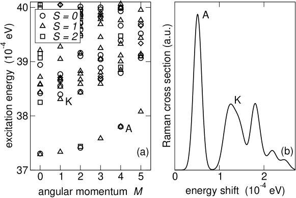
Figure 2: (a) Excitation energies of the four-electron Wigner molecule vs. total orbital angular momentum $M$, for different values of the total spin $S$, with $\lambda=10$. (b) Corresponding Raman scattering cross section for charge excitations in the off-resonance limit. Here we set $\left|\mathbf{q}\right|=2\times 10^{5}$ cm^-1 and introduce a fictitious gaussian broadening of Raman peaks ($\sigma=0.9\times 10^{-5}$ eV). GaAs parameters were used throughout the paper.

First, the two possible spin multiplets other than $S=1$, namely $S=0,2$, lie very close in energy to the ground state. This is understood by invoking electron crystallization. In fact, in the Wigner limit, the Hamiltonian of the system turns into a classical quantity, since the kinetic energy term in it may be neglected with respect to the Coulomb term. Therefore, only commuting operators (the electron positions) appear in the Hamiltonian. In this regime the spin, which has no classical counterpart, becomes irrelevant:[24, 42] spin-dependent energies show a tendency to degeneracy. This can also be understood in the following way: if electrons sit at some lattice sites with unsubstatial overlap of their localized wave functions, then the total energy must not depend on the relative orientation of neighboring spins.

Second, an exact replica of the sequence of the two lowest-energy singlet and triplet states occurs for both $M=0$ and for $M=4$ [(cf. the triplet state labeled A in Fig. 2(a)]. Such a period of four units on the $M$ axis identifies a magic number,[3, 43] whose origin is brought about by the internal spatial symmetry of the interacting wave function.[44, 45] In fact, when electrons form a stable Wigner molecule, they arrange themselves into a four-fold symmetry configuration, where charges are localized at the corners of a square.[31, 46, 47]

A third distinctive signature of crystallization is the appearance of a rotational band,[43] which in Fig. 2(a) is composed of those lowest-energy levels, separated by energy gaps of about $0.1$ meV, that increase monotonically as $M$ increases. This band is called “rotational” since it can be identified with the quantized levels $E_{\mathrm{rot}}(M)$ of a rigid two-dimensional top, given by the formula

$$E_{\mathrm{rot}}(M)=\frac{\hbar^{2}}{2I}M^{2},$$

where $I$ is the moment of inertia of the top.[43] These excitations may be thought of as the “normal modes” of the Wigner molecule rotating as a whole in the $xy$ plane around the vertical symmetry axis parallel to $z$.

Figure 2(b) displays the calculated off-resonance Raman spectrum for charge density fluctuations ($\Delta S=0$, where $\Delta S$ is the variation of the spin with respect to the ground state). The dominant peak is the one labeled A, corresponding to the $\Delta M=4$ normal mode of the Wigner molecule of Fig. 2(a), which therefore represents a clear, visible feature of Wigner crystallization. Notice also the appearance of the so called Kohn mode[1] (labeled K) at higher energy, which is a dipolar ($\Delta M=1$) collective motion of the center of mass of the electron system.

5 Wigner Molecule Formation Seen by Imaging Spectroscopy

Figure 3 shows the QP wave function, corresponding to the injection of the fourth electron into the QD, as a function of $x$ (at $y=0$), for two different values of $\lambda$. As $\lambda$ increases (from 0.5 to 10), the density decreases going from the non-interacting limit ($\lambda=0.5$) deep into the Wigner regime ($\lambda=10$). At high density ($\lambda=0.5$, approximately corresponding to the electron density $n_{e}=3.3\times 10^{12}$ cm^-2) the wave function substantially coincides with the non-interacting FD $p$-like orbital.

Figure 3: Quasi-particle wave function vs. $x$ ($y=0$) for different values of the dimensionless Coulomb-to-kinetic energy ratio $\lambda$. The STS differential conductance, proportional to the wave function square modulus, corresponds to the tunneling process $N=3\rightarrow N=4$. The length unit is the characteristic dot radius $\ell_{\mathrm{QD}}$.

By increasing the QD radius (and $\lambda$), the QP wave function weight moves towards larger values of $r$ (the $s$-like symmetry of the $\lambda=10$ curve comes from a transition of the three-electron ground state[24] around $\lambda\approx 6$). By measuring lengths in units of $\ell_{\mathrm{QD}}$, as it is done in Fig. 3, this trivial effect should be totally compensated. However, we see for $\lambda=10$ ($n_{e}\approx 1.1\times 10^{9}$ cm^-2) that the now much stronger correlation is responsible for an unexpected weight reorganization, which is related to the formation of a “ring” of crystallized electrons in the Wigner molecule (cf. Sec. 4). The shape of the $\lambda=10$ curve of Fig. 3 is consistent with the onset of a solid phase with four electrons sitting at the apices of a square, as discussed in Sec. 4. Note also the dramatic weight loss of QPs as $\lambda$ is increased: the stronger the correlation, the more effective the “orthogonality” between interacting states.

6 Conclusions

The Wigner molecule is an intriguing electron phase, peculiar of QDs, which still lacks for experimental confirmation. We predict that both inelastic light scattering and imaging spectroscopies are able to probe distinctive features of crystallization.

References

- [1] L. Jacak, P. Hawrylak, and A. Wójs, Quantum Dots (Springer, Berlin, 1998).
- [2] T. Chakraborty, Quantum Dots - A Survey of the Properties of Artificial Atoms (North-Holland, Amsterdam, 1999).
- [3] P. A. Maksym and T. Chakraborty, Phys. Rev. Lett. 64, 108 (1990).
- [4] M. A. Kastner, Phys. Today 46 (March), 24 (1993).
- [5] R. Ashoori, Nature 379, 413 (1996).
- [6] S. Tarucha, D. G. Austing, T. Honda, R. J. van der Hage, and L. P. Kouwenhoven, Phys. Rev. Lett. 77, 3613 (1996).
- [7] M. Rontani, G. Goldoni, and E. Molinari, in New directions in mesoscopic physics (towards nanoscience), ed. R. Fazio et al., NATO Science Series II: Physics and Chemistry 125, 361 (2003).
- [8] M. Rontani, F. Rossi, F. Manghi, and E. Molinari, Appl. Phys. Lett. 72, 957 (1998).
- [9] C. P. García, V. Pellegrini, A. Pinczuk, M. Rontani, G. Goldoni, E. Molinari, B. S. Dennis, L. N. Pfeiffer, and K. W. West, Phys. Rev. Lett. 95, 266806 (2005).
- [10] D. G. Goldhaber-Gordon, H. Shtrikman, D. Mahalu, D. Abusch-Magder, U, Meirav, and M. A. Kastner, Nature 391, 156 (1998).
- [11] S. M. Cronenwett, T. H. Oosterkamp, and L. P. Kouwenhoven, Science 281, 540 (1998).
- [12] S. M. Reimann and M. Manninen, Rev. Mod. Phys. 74, 1283 (2002).
- [13] M. Rontani, S. Amaha, K. Muraki, F. Manghi, E. Molinari, S. Tarucha, and D. G. Austing, Phys. Rev. B 69, 85327 (2004).
- [14] T. Ota, M. Rontani, S. Tarucha, Y. Nakata, H. Z. Song, T. Miyazawa, T. Usuki, M. Takatsu, and N. Yokoyama, Phys. Rev. Lett. 95, 236801 (2005).
- [15] H. Grabert and M. H. Devoret (eds.), Single charge tunneling, NATO ASI series B: Physics 294 (Plenum, New York, 1992).
- [16] N. Kirstaedter et al., Electron. Lett. 30, 1416 (1994).
- [17] H. L. Edwards, Q. Niu, G. A. Georgakis, and A. L. de Lozanne, Phys. Rev. B 52, 5714 (1995).
- [18] X. Michalet et al., Science 307, 538 (2005).
- [19] D. Loss and D. P. DiVincenzo, Phys. Rev. A 57, 120 (1998).
- [20] M. Rontani, F. Troiani, U. Hohenester, and E. Molinari, Solid State Commun. 119, 309 (2001).
- [21] G. Bastard, Wave mechanics applied to semiconductor heterostructures (Les Editions de Physique, Les Ulis, 1998).
- [22] L.-W. Wang and A. Zunger, Phys. Rev. B 59, 15806 (1999).
- [23] R. Egger, W. Häusler, C. H. Mak, and H. Grabert, Phys. Rev. Lett. 82, 3320 (1999).
- [24] Full details on our algorithm and its perfomances in M. Rontani, C. Cavazzoni, D. Bellucci, and G. Goldoni, J. Chem. Phys. (2006), available also as cond-mat/0508111.
- [25] See the code website http.//www.s3.infm.it/donrodrigo.
- [26] G. Abstreiter, M. Cardona, and A. Pinczuk, in Light scattering in solids IV, eds. M. Cardona and G. Güntherodt (Springer-Verlag, Berlin, 1984), p. 5.
- [27] D. J. Lockwood, P. Hawrylak, P. D. Wang, C. M. Sotomayor Torres, A. Pinczuk, and B. S. Dennis, Phys. Rev. Lett. 77, 354 (1996).
- [28] C. Schüller, K. Keller, G. Biese, E. Ulrichs, L. Rolf, C. Steinebach, D. Heitmann, and K. Eberl, Phys. Rev. Lett. 80, 2673 (1998).
- [29] T. Brocke, M.-T. Bootsmann, M. Tews, B. Wunsch, D. Pfannkuche, Ch. Heyn, W. Hansen, D. Heitmann, and C. Schüller, Phys. Rev. Lett. 91, 257401 (2003).
- [30] P. Hawrylak, Solid State Commun. 93, 915 (1995).
- [31] M. Rontani, G. Goldoni, F. Manghi, and E. Molinari, Europhys. Lett. 58, 555 (2002).
- [32] B. Grandidier, Y. M. Niquet, B. Legrand, J. P. Nys, C. Priester, D. Stiévenard, J. M. Gérard, and V. Thierry-Mieg, Phys. Rev. Lett. 85, 1068 (2000).
- [33] E. E. Vdovin, A. Levin, A. Patanè, L. Eaves, P. C. Main, Yu. N. Khanin, Yu. V. Dubrovskii, M. Henini, and G. Hill, Science 290, 122 (2000).
- [34] O. Millo, D. Katz, Y. Cao, and U. Banin, Phys. Rev. Lett. 86, 5751 (2001).
- [35] T. Maltezopoulos, A. Bolz, C. Meyer, C. Heyn, W. Hansen, M. Morgenstern, and R. Wiesendanger: Phys. Rev. Lett. 91, 196804 (2003).
- [36] O. S. Wibbelhoff, A. Lorke, D. Reuter, and A. D. Wieck, Appl. Phys. Lett. 86, 092104 (2005).
- [37] D. Reuter, P. Kailuweit, A. D. Wieck, U. Zeitler, O. Wibbelhoff, C. Meier, A. Lorke, and J. C. Maan, Phys. Rev. Lett. 94, 026808 (2005).
- [38] M. Rontani and E. Molinari, Phys. Rev. B 71, 233106 (2005).
- [39] M. Rontani and E. Molinari, Jpn. J. Appl. Phys. (2006) [cond-mat/0507688].
- [40] J. Bardeen, Phys. Rev. Lett. 6, 57 (1961).
- [41] J. Tersoff and D. R. Hamann, Phys. Rev. B 31, 805 (1985).
- [42] M. Rontani, C. Cavazzoni, and G. Goldoni, Computer Physics Commun. 169, 430 (2005).
- [43] M. Koskinen, M. Manninen, B. Mottelson, and S. M. Reimann, Phys. Rev. B 63, 205323 (2001).
- [44] W. Y. Ruan, Y. Y. Liu, C. G. Bao, and Z. Q. Zhang, Phys. Rev. B 51, 7942 (1995).
- [45] P. A. Maksym, H. Imamura, and G. P. Mallon, J. Phys.: Condens. Matter 12, R299 (2000).
- [46] F. Bolton and U. Rössler, Superlatt. Microstruct., 13, 139 (1993).
- [47] V. M. Bedanov and F. M. Peeters, Phys. Rev. B 49, 2667 (1994).