Quantum Adiabatic Evolution Algorithm and Quantum Phase Transition in 3-Satisfiability Problem

Abstract

In this paper we show that the performance of the quantum adiabatic algorithm is determined by phase transitions in underlying problem in the presence of transverse magnetic field $\Gamma$. We show that the quantum version of random Satisfiability problem with 3 bits in a clause (3-SAT) has a first-order quantum phase transition. We analyze the phase diagram $\gamma=\gamma(\Gamma)$ where $\gamma$ is an average number of clauses per binary variable in 3-SAT. The results are obtained in a closed form assuming replica symmetry and neglecting time correlations at small values of the transverse field $\Gamma$. In the limit of $\Gamma=0$ the value of $\gamma(0)\approx$ 5.18 corresponds to that given by the replica symmetric treatment of a classical random 3-SAT problem. We demonstrate the qualitative similarity between classical and quantum versions of this problem.

I Introduction

From the early years of computing it was realized that some problems are inherently intractable. This intuition has been quantified by the theory of computational complexity proposed by Cook cook . Most problems of practical interest can be roughly divided into two classes: P and NP-complete. Problems in the former class can be solved on a computer in time that scales only polynomially with the size of an instance of the problem. Solution to NP-complete problems can be verified in polynomial time, but it is believed that it cannot be found in polynomial time on a classical computer. Solving NP-complete problem typically requires exponential time which makes then intractable. All NP-complete problems are equivalent; if it were possible to solve one NP-complete problem in polynomial time, it would be possible to apply the same algorithm to solve all NP-complete problems.

It is not known yet whether NP-complete problems can be solved efficiently on a quantum computer. Shor’s algorithm shor for a quantum computer can solve in polynomial time the number factoring problem that is presumably hard for a classical computer. It is not, however, in the NP-complete class (and its decision variant is in P).

Just as research in classical computing focus on worst-case complexity has been superseded by the analysis of typical case complexity and application of general-purpose algorithms like simulated annealing, similar changes take place in the field of quantum computing. A substantial interest has been generated by a general-purpose quantum adiabatic algorithm (QAA) proposed by Farhi and coworkers farhi ; FarhiSc .

In its simplest form QAA is applied to problems where underlying variables can have only two values, and a solution is given by a N-bit binary string. It corresponds to a time-dependent Hamiltonian that slowly changes from a simple form (for which the ground state can be constructed exactly) to a complex form that describes an instance of NP-complete problem. The initial Hamiltonian is typically chosen to correspond to a uniform magnetic field $\Gamma$ applied along $\hat{x}$ direction

$$H_{\textrm{in}}=-\Gamma\sum_{i=1}^{N}\hat{\sigma}_{i}^{x},$$ (1)

so that the ground state in $\{\hat{\sigma}_{i}^{z}\}$ basis is a symmetric superposition of $2^{N}$ binary vectors

$$\psi_{\textrm{in}}=\frac{1}{2^{N/2}}\sum_{\{s_{i}=\pm 1\}}|s_{1}s_{2}\cdots s_{N}\rangle.$$ (2)

The final Hamiltonian is chosen to be diagonal in $\{\hat{\sigma}_{i}^{z}\}$ basis with diagonal elements corresponding to the cost function values for particular assignments of binary variables $\{s_{i}\}$

$$H_{\rm fin}=\sum_{\{s_{i}\}}E[\{s_{i}\}]|s_{1}s_{2}\cdots s_{N}\rangle\langle s_{1}s_{2}\cdots s_{N}|.$$ (3)

At intermediate times the Hamiltonian is a linear combination of initial and final Hamiltonians. We choose to write this in the following form

$$H=\sum_{\{s_{i}\}}E[\{s_{i}\}]|s_{1}\cdots s_{N}\rangle\langle s_{1}\cdots s_{N}|-\Gamma\sum_{i}\widehat{\sigma}_{i}^{x}.$$ (4)

In the beginning of the algorithm $\Gamma\rightarrow\infty$ so that the second term dominates and a ground state has a simple form. At the end of the algorithm $\Gamma=0$ and the ground state corresponds to a solution of the NP-complete problem that minimizes cost function. If $\Gamma$ is lowered sufficiently slowly, adiabatic theorem tells us that the system will remain in its ground state with a high probability. The second term is referred to as a driver term because its presence in otherwise diagonal Hamiltonian is to enable spin flips. The algorithm is quite similar to the simulated annealing (SA) algorithm in this respect. In QAA transverse field $\Gamma$ replaces temperature $T$. The dynamics of these two problems are quite different.

The fundamental limitation of the SA algorithm is the critical slowing down at the point of classical phase transition. The system may become trapped in one of the local minima surrounded by high barriers and that requires exponentially long time to escape. For the QAA the metric of the algorithm performance can be given in terms of the eigenstates $\Psi_{k}(\Gamma)$ and eigenvalues $E_{k}(\Gamma)$ of the interpolating Hamiltonian $H(\Gamma)$. The rate at which $\Gamma(t)$ can be lowered obeys the strong inequality $\hbar|\dot{\Gamma}(t)|\langle\Psi_{0}|\,dH/d\Gamma|\Psi_{0}\rangle\ll(E_{1}(\Gamma)-E_{0}(\Gamma))^{2}$. A sufficient condition for the success of QAA requires a polynomial scaling with the problem size $N$ of a minimum gap $\Delta E_{\rm min}=\min_{\,\Gamma\in(0,\infty)}\left(E_{1}(\Gamma)-E_{0}(\Gamma)\right)$ between the two lowest energy levels of $H(\Gamma)$. The danger is that there are points of avoided crossing ((see Fig. 1)) at which the gap can be exponentially small.

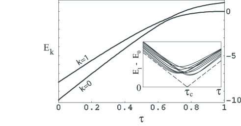
Figure 1: Two lowest eigenvalues of the Hamiltonian $H$ (4) vs the interpolating parameter $\tau=1/(1+\Gamma)$. In simulations $H_{\rm fin}$ corresponds to a randomly generated instance of the version of Satisfiability problem Exact Cover FarhiSc with the number of bits $N$=10. Insert: different plots show the $\tau$-dependencies of the gap between the two lowest eigenvalues of $H$ for various random instances of Exact Cover with $N$=10. Dashed lines indicate the approximate asymptotical position of the avoided-crossing point in the limit $N\rightarrow\infty$.

At such point the branches of $E_{0}(\Gamma)$ correspond to wavefunctions with exponentially small overlap. This effect has been demonstrated analytically in a toy problem Vazirani02 ; qaetoy as well as for the case of NP-complete problem Positive-1-in-K-sat with large number of bits in a clause, $K\gg 1$ skm:04 .

An equivalent measure of the algorithmic complexity is the second derivative of the ground state energy $\mathrm{d}^{2}E_{0}/\mathrm{d}\Gamma^{2}$. This quantity can become exponentially large at the point of avoided crossing where it is $\propto 1/\Delta E_{\rm min}$. If the minimum gap $\Delta E_{\rm min}$ shrinks to zero in the thermodynamic limit $N\rightarrow\infty$ for some $\Gamma=\Gamma_{c}$ then the ground state energy $E_{0}(\Gamma)$ possesses a cusp (cf. Fig. 1). This cusp signals a first-order quantum phase transition. Indeed, the ground state energy is precisely the free energy in the limit $\beta=1/T\rightarrow\infty$:

$$E_{0}(\Gamma)\equiv\lim_{\beta\rightarrow\infty}F(\beta,\Gamma)=-\lim_{\beta\rightarrow\infty}\frac{1}{\beta}\ln\textrm{Tr}\left\{e^{-\beta\hat{H}(\Gamma)}\right\}.$$ (5)

Time evolution has to be slowest at the point of the first-order quantum phase transition, reminiscent of a critical slowing down at the point of classical phase transition.

We will be working with an ensemble of random instances of NP-complete problem and recast it as essentially a spin glass model. Although quantum phase transitions in infinitely-connected models of spin glasses have been extensively studied qsg1 ; dynamic ; dynamic2 ; dynamic3 , there are no results to our knowledge on dilute quantum spin glasses. At the same time most of NP-complete problems are closely related to dilute spin glass models.

The central quantity we will be computing is the disorder-averaged (instance-averaged) free energy $\langle F(\beta)\rangle$. We will classify the quantum phase transition as random first-order or random second-order as deduced from the non-analyticity in $\langle F\rangle$ vs $\Gamma$. In classical case, random first-order phase transition is typically associated with exponentially hard problems. It is therefore tempting to suggest that the onset of the first-order quantum phase transition is indicative of the exponential, or stretched-exponential Fisher ; Reichardt scaling law of the runtime of QAA with $N$ determined by the distribution of the tunnelling times between the valleys of an energy landscape.

Within current formalism we are limited to this qualitative picture. The determination of the minimum gap requires more elaborate methods. One would naively expect that finite-size scaling analysis can be used to derive the scaling of the minimum gap with $N$. Observe though that, if disorder is relevant and assuming the first-order phase transition, the position of the minimum gap fluctuates with disorder around some value $\Gamma_{c}$ (see Fig. 1). If we fix a value of $\Gamma$ and perform the disorder-average, we will have $\langle E_{1}(\Gamma)-E_{0}(\Gamma)\rangle\gtrsim O(1/\sqrt{N})$. Minimized over $\Gamma$, it is still $O(1/\sqrt{N})$ even though true minimum gap can be arbitrarily small.

The paper is organized as follows. In Sec. II we introduce the random K-SAT problem – the model that we study in this paper. In Sec. III we describe exact results from the random graph theory and empirical results on satisfiability transition. K-SAT problem has been extensively studied in the classical limit for zero temperature. This section is devoted to these results as well as effects of finite temperature. The Sec. IV formulates the K-SAT problem in quantum case in the presence of transverse magnetic field. Subsequently two approximations are made to make the problem tractable: the so-called replica-symmetric ansatz that assumes absence of long-range correlations is made, and the static ansatz that assumes that any correlations time correlations are due to the transverse magnetic field alone. The expression for the free energy and the self-consistency equation for the order parameter are derived. In the Sec. V we consider the limit of small transverse magnetic field $\Gamma$ and derive the simplified self-consistency equations for this case. Sec. VI is Conclusion.

II K-SAT Problem

As a test case for QAA algorithm we consider the satisfiability problem that happens to be the first problem to be associated with NP-complete class cook . More precisely, we will work with a variant of satisfiability problem – the K-SAT that places a constraint on the number of variables that can appear in a clause. The K-SAT is known to be NP-complete for $K\geqslant 3$. This means that any NP-complete problem can be reformulated as an instance of 3-SAT. We will concentrate on this particular case ($K=3$). The benefits of working with K-SAT is that the problem Hamiltonian is local (K-local to be exact, but can easily be recast as a 2-local Hamiltonian; see qaesolid for application to QAA algorithm); and also that random K-SAT is intrinsically related to random hypergraphs and is amenable to methods of statistical physics.

An instance of K-SAT is a boolean formula in conjunctive normal form (CNF), i.e. a set of clauses

$$\mathcal{F}=\mathcal{C}_{1}\wedge\mathcal{C}_{2}\wedge\cdots\wedge\mathcal{C}_{M}$$ (6)

where each clause represents a logical OR of $K$ literals, each literal representing either one of the variables $x_{1},\ldots,x_{N}$ or a its logical NOT. Below is an example of possible K-SAT clause for $K=3$:

$$x_{2}\vee\bar{x}_{5}\vee\bar{x}_{11}$$ (7)

(where $\bar{x}$ represents logical NOT of $x$).

The formula is said to be satisfiable if and only if there exists an assignment of boolean variables $\{x_{i}\}$ such that all $M$ clauses comprising a formula are satisfied (evaluate to true) at the same time. Presented with an instance of K-SAT formula, algorithm must determine if it is satisfiable and if it is, find the appropriate assignment of variables.

We follow the standard recipe for trivial mapping of constraint satisfaction problems to problems in statistical mechanics by defining the energy function to be proportional to the number of violated clauses. The constant of proportionality is chosen to be $2$. The motivation for this choice will become evident later. The energy can be written as follows

$$E=2\sum_{m}\theta(J_{m1}s_{i_{m1}})\theta(J_{m2}s_{i_{m2}})\cdots\theta(J_{mK}s_{i_{mK}}).$$ (8)

where we replaced boolean variables with spins $s_{i}=\pm 1$, the value $s=-1$ corresponding to true. $\theta(x)$ is the Heaviside function $\theta(x)=1$ if $x>0$ and $\theta(x)=0$ if $x\leqslant 0$. Variables $i_{m1},\ldots.,i_{mK}$ are indices of variables that appear in a clause, and $J_{m1},\ldots,J_{mK}=\pm 1$ describe whether the literal that appears in a clause is negated ($J=-1$).

We will work with an ensemble of random instances of K-SAT with fixed number of variables $N$, number of clauses $M$ and number variables per clause $K$. This merely means that indices $i_{mp}$ are independent and drawn uniformly at random from the set $1,2,\ldots,N$ and variables $J_{mp}$ are independent random variables that are equal to $+1$ or $-1$ with probability 50 % .

The formula is satisfiable if the ground state energy equals zero, and it is unsatisfiable if it is greater than zero.

The following phenomenon has been discovered satunsat . If we fix the ratio of clauses to variables $\gamma=M/N$, the energy is almost surely $0$ for $\gamma<\gamma_{c}$ in the limit $N\rightarrow\infty$ and $E>0$ for $\gamma>\gamma_{c}$. The value of $\gamma_{c}$ is independent of $N$ in the limit of large $N$, apart from small corrections. Note that the ground state remains exponentially degenerate across the transition. The exact value of $\gamma_{c}$ is an interesting problem in combinatorics mathconst ; rigorous determination of $\gamma_{c}$ has not yet been accomplished.

The threshold phenomena in random graphs were known since pioneering work of Erdos and Renyi erdos . Random K-SAT problem has intimate connections to the theory of random graphs. One can picture an instance of random K-SAT as a random hypergraph. Variables correspond to vertices of the hypergraph and clauses correspond to hyperedges that join $K$ vertices. One threshold phenomenon that was examined in erdos in the context of random graphs but can be extended to random hypergraphs, is the appearance of giant component. In physics it is known as percolation transition. When $\gamma<1/K(K-1)$ a random hypergraph is with high probability is a collection of disjoint clusters of typical size $O(1)$, with the largest cluster not exceeding $O(\log N)$ in size. All clusters (with few (i.e. $O(1)$) exceptions) have a form of trees, that is contain no loops. For $\gamma>1/K(K-1)$ the same picture holds, but there appears a giant (of size $O(N)$) supercluster. The structure of the giant supercluster is very complex. It contains a large number of loops, but the length of these loops is relatively large: $O(\log N)$. It is in the giant supercluster that the complexity of the problem is buried. Indeed, small isolated clusters can be efficiently tackled using divide-and-conquer approach. Moreover, since they are all tree-like, the assignment of variables that satisfies corresponding clauses always exists and can be found in linear time.

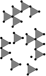
Figure 2: Example of hypergraph corresponding to random instance of 3-SAT. Vertices represent variables and traingles represent clauses involving $K=3$ variables.

Although phase transition is evident in geometric properties, owing to long length of the loops in the supercluster, no abnormal behavior in the space of solutions is seen immediately following the phase transition. The formula remains satisfiable well past the percolation transition, nor any correlations between spins in the supercluster that are far away from each other are detected. One must note that such correlations do appear at so called dynamic transition $\gamma_{d}$, at which point finding the solution becomes difficult (for simulated annealing algorithm).

Figure 3: Complexity of the instance as the function of $\gamma=M/N$. Problem becomes exponentially hard for $\gamma>\gamma_{d}$ and the complexity peaks at satisfiability threshold $\gamma_{c}$.

The performance of algorithm is subject to similar threshold phenomenon. Typically, algorithms require just a polynomial (often linear) time for $\gamma$ less than some critical value $\gamma_{d}$ and require an exponential time for $\gamma>\gamma_{d}$. One can introduce the normalized complexity $\lim_{N\rightarrow\infty}\frac{1}{N}\log T$, where $T$ is the time it takes to solve a problem (units of $T$ are unimportant in $N\rightarrow\infty$ limit since the logarithm is taken). It is a self-averaging quantity and hence a function of $\gamma$ alone (in the usual sense, with high probability a random formula has this complexity). This function equals zero for $\gamma<\gamma_{d}$ and for $\gamma>\gamma_{d}$ it is non-zero. The exact value of $\gamma_{d}$ and the shape of the complexity function is not universal, but rather algorithm-dependent. Simulations suggests that for most common algorithm the complexity peaks at $\gamma_{c}$ that is the point SAT/UNSAT transition. Indeed, the satisfiability threshold is the place where one intuitively expects to find the hardest (and most interesting) problems. The exact determination of the complexity function is invaluable as a non-empirical means for comparing the asymptotic efficiency of various algorithm. This is particularly useful in the field of quantum computing, where empirical research is impossible since no prototype of quantum computer exist and its simulation on classical computer is not feasible for large instances of the problem. An important benchmark of the algorithm is $\gamma_{d}$ itself (larger is better) as it marks a region where the problem can be solved very efficiently. An alluring (but not necessarily impossible) goal is designing an algorithm that has $\gamma_{d}\geqslant\gamma_{c}$.

Although the value of $\gamma_{d}$ is algorithm-dependent, a particular value that we denote $\gamma_{\textrm{RSB}}$ is universal in a sense that it should be the same for all local search algorithms. It corresponds to the point where the energy landscapes qualitatively changes. There appears an exponentially large number of local minima, i.e. a set of states corresponding to $E=0$ becomes disconnected. In contrast for $\gamma<\gamma_{\textrm{RSB}}$ a set of states with $E=0$ is connected. This transition can be seen in the behavior of the free energy. This is the point where so-called replica-symmetric ansatz breaks down. This will be elaborated on in the next section.

III Review of Classical Result

In a number of articles ksat1 ; ksat2 ; ksat3 ; ksat4 ; ksat5 satisfiability transition has been studied in K-SAT problem using replica method. Statistical properties of physical system are completely determined by its free energy

$$F=-T\ln Z=-T\ln\sum_{\{s_{i}\}}\mathrm{e}^{-\beta H[\{s_{i}\}]}.$$ (9)

If the Hamiltonian depends on the disorder, we must also average the free energy over disorder configurations. Note that it is not appropriate to attempt to compute the disorder average of $Z$. Indeed $Z$ is exponentially large and small $o(N)$ fluctuations of $F$ amplify in $Z=\mathrm{e}^{-\beta F}$. Therefore

$$\langle Z\rangle=\left\langle\mathrm{e}^{-\beta F}\right\rangle\neq\mathrm{e}^{-\beta\langle F\rangle}.$$ (10)

Note that although the free energy $F$ is $O(N)$, fluctuations due to disorder are only $O(\sqrt{N})$ and can be neglected in the thermodynamic limit. Disorder averaging of $F$ is just a useful trick, since to the leading order in $N$, same value should be obtained for $F$ for almost all possible disorder realizations (all but a fraction that goes to $0$ with increasing $N$).

Replica method accomplishes the averaging as follows. $n$ non-interacting copies of the system are prepared, all having the identical disorder configuration. This is indicated by attaching an additional replica index $\alpha=1,\ldots,n$ to each variable $s_{i}$; new variables are labeled $s_{i}^{\alpha}$. The partition function of such system equals $Z^{n}$, where $Z$ is the partition function of non-replicated system. Disorder average of the replicated system is then performed, which is easy to accomplish since summation over all possible spin configurations $\{s_{i}^{\alpha}\}$ can be done after the disorder averaging, which eliminates the difficulty of computing the partition function that explicitly depends on the disorder. Once analytical expression for $\langle Z^{n}\rangle$ is obtained, the disorder-averaged free energy $\langle F\rangle=-T\langle\ln Z\rangle$ is computed via analytical continuation using the identity

$$\langle\ln Z\rangle=\left.\frac{\mathrm{d}}{\mathrm{d}n}\langle Z^{n}\rangle\right|_{n=0}$$ (11)

The Hamiltonian for the K-SAT problem has been introduce in the previous section (Eq. 8). In the limit of zero temperature satisfiable phase is characterized by $\langle E\rangle=0$; in the unsatisfiable (UNSAT) phase $\langle E\rangle>0$.

In the simplest approximation it is assumed that the symmetry of the Hamiltonian with respect to the interchange of replica indices $\alpha$ is not spontaneously broken. The physical interpretation of this is the absence of long-range correlations. For randomly chosen variables $s_{i}$ and $s_{j}$, replica symmetric ansatz implies

$$\langle s_{i}s_{j}\rangle=\langle s_{i}\rangle\langle s_{j}\rangle$$ (12)

(randomly chosen sites are with high probability at least $O(\log N)$ away from each other; correlations are absent in the limit $N\rightarrow\infty$).

Owing to identity (12) statistical properties (correlations) in the thermodynamic limit are completely determined by specifying average magnetizations of individual spins $m_{i}=\langle s_{i}\rangle$. The order parameter of the system is the histogram of magnetizations of spins $P(m)$. In practice it is convenient to define effective fields $h_{i}=T\tanh^{-1}m_{i}$ and choose the histogram of effective fields as an order parameter. An expression for the free energy can be written out in terms of $P(h)$.

$$F = \frac{1}{\beta}\int\mathrm{d}h\ln(2\cosh\beta h)\int\frac{\mathrm{d}\omega}{2\pi}\tilde{P}(\omega)(\ln\tilde{P}(\omega)-1)$$ (13)

$$-\frac{\gamma}{\beta}\int\prod_{i=1,2,3}\mathrm{d}h_{i}P(h_{i})\ln\left[1-\frac{1-\mathrm{e}^{-\beta}}{\prod_{i=1,2,3}(1+\mathrm{e}^{2\beta h_{i}})}\right]$$

Varying this expression with respects to $P(h)$ yields a self-consistency equation of $P(h)$ which can be solved numerically. This equation is essentially an iterative procedure for determining correct magnetic fields for clusters without loops (trees) combined with the Poisson distribution for the number of branches in a random tree.

For high connectivities $\gamma$ and low temperatures $T$ solution to the self-consistency equation yields two solutions. A solution that maximizes the free energy should be chosen. Note that this is in contrast to standard of choosing a solution with the smaller free energy for first-order phase transition in pure systems. This reversal is standard feature of replica method and the rationale is discussed in sgbook .

For zero temperature the solution is drastically simplified. $P(h)$ has the form of a series of delta-function peaks at integer values of $h$

$$P(h)=\sum_{k}p_{k}\delta(h-k).$$ (14)

These magnetic fields can be interpreted as follows. Non-zero values of $h$ ($|h|\geqslant 1$) correspond to frozen variables. Indeed $h_{i}\geqslant 1$ corresponds to $m_{i}=+1$ and $h_{i}\leqslant-1$ corresponds to $m_{i}=-1$. The appearance of finite fraction of such frozen spins, or backbone, signals the beginning of unsatisfiable phase. The absolute value of $h_{i}$ ($|h_{i}|$) then indicates the increase in the number of violated clauses if the frozen spin is flipped.

Since the problem is symmetric with respect to sign flip $s_{i}\rightarrow-s_{i}$, $P(h)$ is necessarily symmetric. Introduce variable $q$

$$q=\sum_{k=1}^{\infty}p_{k}$$ (15)

Then obviously $p_{0}=1-2q$ since all $p_{k}$’s must add up to $1$. The self-consistency equation can be written in the following form

$$1-2q = \mathrm{e}^{-3\gamma q^{2}}I_{0}(3\gamma q^{2})$$ (16)

$$p_{k} = \mathrm{e}^{-3\gamma q^{2}}I_{k}(3\gamma q^{2})$$ (17)

Equivalently, these equations can be derived as follows duxbury . Let the fraction of frozen variables be $2q$, with half of these being polarized to $+1$ and another half to $-1$. Next, we add $N+1$-st (cavity) spin to the system together with extra clauses. The number of extra clauses is Poisson-distributed with parameter $3\gamma$. Each extra clause involves a cavity spin and two randomly chosen variables of $N$-spin system. The clause forces a certain value for the cavity spin only if both variables other than a cavity spin are frozen to a value that equals corresponding $J_{mi}$. The probability of this occurrence is $q^{2}$. Every such clause gives a contribution $u=J_{m1}$ to the effective field $h$ of cavity spin. This contribution is $+1$ or $-1$ with probability of 50 % each. If the probability that the clause contributes $u=+1$ (or $u=-1$) is $q^{2}/2$, the number of clauses attached to cavity spin that contribute $u=+1$ (or $u=-1$) is Poisson with parameter $\frac{3}{2}\gamma q^{2}$. Therefore, we can write the probability that the effective field of the cavity spin is $k$:

$$p_{k}=\sum_{l,m}\frac{(3\gamma q^{2}/2)^{l}}{l!}\frac{(3\gamma q^{2}/2)^{m}}{m!}\mathrm{e}^{-3\gamma q^{2}}\delta_{l-m,k}$$ (18)

The right-hand side is evaluated to be $\mathrm{e}^{-3\gamma q^{2}}I_{k}(3\gamma q^{2})$. When the effective field equals zero, the cavity spin is not frozen. Since the properties of $N$-spin system and $N+1$-spin system should not differ in the thermodynamic limit, the probability of this is $1-2q$. Thus we obtain the self-consistency equation on $q$.

$$1-2q=\mathrm{e}^{-3\gamma q^{2}}I_{0}(3\gamma q^{2}).$$ (19)

This equation does not determine $q$ uniquely; when both trivial solution ($q=0$) and a non-trivial ($q\neq 0$) are present, the correct value of $q$ is chosen by examining the expression (13) for the free energy and choosing a solution that maximizes the free energy. Although a non-trivial solution appears at $\gamma\approx 4.67$, it does not become stable until $\gamma_{c}\approx 5.18$

At finite but small temperature this picture is modified as follows. A series of delta-function peaks in $P(h)$ are broadened and acquire a finite $O(T)$ width (similar broadening occurs in quantum case for small $\Gamma$, see figure 6). The values of $q$ and integrated probability weights around integer values of $h$ remain the same. Effective fields for spins that are not frozen $h\approx 0$ acquire $O(T)$ corrections so that the magnetization $m=\tanh\beta h=O(1)$ and spins in the backbone ($|h|\gtrsim 1$) acquire $O(T)$ correction because of clauses connected to the backbone (see figure 7).

Examination of the free energy also shows that the value of $\gamma_{c}(T)$ increases with increasing temperature. The following phase diagram is obtained.

Figure 4: Simple phase diagram obtained within RS ansatz

Unfortunately, the predicted value of $T=0$ UNSAT transition of $\gamma_{c}\approx\ldots.$ is far from the experimental value of $\gamma_{c}\approx 4.2$. The reason for the discrepancy is that the replica-symmetric ansatz breaks down well before the satisfiability transition. Using an improved 1-step replica-symmetry breaking ansatz (1-step RSB) the break-down of replica symmetry is put at $\gamma_{d}\approx 3.92$ and the satisfiability transition is computed to occur at $\gamma_{c}\approx 4.27$ ksat2 ; ksat5 .

The central assumption of RSB ansatz is that for $\gamma>\gamma_{d}$ the ground state (set of all satisfying assignments) is broken in an exponentially large number of isolated islands separated by large barriers. The identity $\langle s_{i}s_{j}\rangle=\langle s_{i}\rangle\langle s_{j}\rangle$ no longer holds unless the thermal average is restricted to a particular local minimum (or pure state in statistical physics lingo). Rather than being described by individual magnetizations $m_{i}$, the system ought to be described by a histogram of magnetizations taken over all possible pure states $\alpha$. At the level if 1-step RSB, the following identity holds in the thermodynamic limit. For sites $i$ and $j$ chosen at random (and as a result, typically infinitely far away from each other) $P(m_{i}m_{j})=P(m_{i})P(m_{j})$, where $P(m_{i})$ is a histogram of magnetizations at site $i$, and $P(m_{i},m_{j})$ is a histogram of pairs of magnetizations at sites $i$ and $j$.

Note that this ansatz is broken when once one goes beyond single step of replica symmetry breaking. However, it is widely believed to be exact up to $\gamma=\gamma_{c}$; thereafter, additional steps of RSB are required.

Due to the complex nature of the ground state in RSB phase, simulated annealing algorithm should take an exponentially long time to converge to a solution (although other specially designed algorithms can still work efficiently for $\gamma>\gamma_{d}$). A correct phase diagram should take the following form. The exponential slowing down that affects the performance of simulated annealing algorithm occurs at RS/RSB boundary.

Figure 5: Correct phase diagram obtained by considering effects of replica symmetry breaking (RSB). RSB phase separate “easy” and unsatisfiable phases.

IV Quantum 3-SAT

For quantum adiabatic evolution algorithm, the original Hamiltonian is rewritten with operator $\hat{\sigma}_{i}^{z}$ replacing classical spins $s_{i}$ and a driver term $-\Gamma\Sigma_{i}\hat{\sigma}_{i}^{x}$ is added

$$\hat{H}=\hat{H}_{\textrm{cl}}[\{\hat{\sigma}_{i}^{z}\}]-\Gamma\sum_{i}\hat{\sigma}_{i}^{x}.$$ (20)

We expect level crossings and a critical slowing down to occur at phase transition indicated by non-analyticities of quantum partition function

$$Z=\textrm{Tr}\mathrm{e}^{-\beta\hat{H}}$$ (21)

Note that we will let $\beta\rightarrow\infty$ and examine the behavior of $Z$ as a function of transverse field $\Gamma$.

To evaluate the partition function we use the Trotter lattice. Equation (21) can be rewritten as

$$Z=\textrm{Tr}\left[\mathrm{e}^{-(\beta/M)\hat{H}_{\textrm{cl}}[\{\hat{\sigma}_{i}^{z}\}]+(\beta\Gamma/M)\sum_{i}\hat{\sigma}_{i}^{x}}\right]^{M}$$ (22)

We can use Baker’s identity

$$\mathrm{e}^{\hat{A}+\hat{B}}=\mathrm{e}^{\hat{A}}\mathrm{e}^{\hat{B}}\mathrm{e}^{-\frac{1}{2}[\hat{A},\hat{B}]+\cdots}$$ (23)

where additional terms involve higher-order commutators. In our case both $\hat{A}$ and $\hat{B}$ are $O(1/M)$ hence the last term in (23) is $\mathrm{e}^{O(1/M^{2})}$ and does not contribute to (22) in the limit $M\rightarrow\infty$.

$$Z=\textrm{Tr}\left[\mathrm{e}^{-(\beta/M)\hat{H}_{\textrm{cl}}[\{\hat{\sigma}_{i}^{z}\}]}\mathrm{e}^{(\beta\Gamma/M)\sum_{i}\hat{\sigma}_{i}^{x}}\right]^{M}.$$ (24)

To evaluate this expression for each of $M$ factors we insert basis states corresponding to all $2^{N}$ projections of $\hat{\sigma}_{i}^{z}$. We denote basis states by vector $s_{i,t}$ where $t=0,\ldots,M$ labels a factor in which the basis states appear. Since we are taking a trace we are imposing a periodicity condition $s_{i,0}=s_{i,M}$. Since $\hat{H}_{\textrm{cl}}$ is obviously diagonal in this basis, first term is simply written as

$$\mathrm{e}^{-(\beta/M)H_{\textrm{cl}}[\{s_{i,t}\}]}$$ (25)

and using $\mathrm{e}^{a\hat{\sigma}^{x}}=\textrm{ch}a+\hat{\sigma}^{x}\textrm{sh}a$, second term can be written as

$$\left(\operatorname{ch}\frac{\beta\Gamma}{M}\right)^{N}\mathrm{e}^{\ln\operatorname{th}(\beta\Gamma/M)\sum_{i}(1-s_{i,t}s_{i,t+1})/2}.$$ (26)

The partition function of system with $N$ quantum spins is thus written effectively as a partition function of classical system with $NM$ classical spins.

$$Z=(\operatorname{ch}\Gamma\Delta t)^{NM}\sum_{\{s_{i,t}\}}\mathrm{e}^{-\Delta t\sum_{t}H_{\operatorname{cl}}[\{s_{i,t}\}]+\ln\operatorname{th}(\Gamma\Delta t)\sum_{i,t}(1-s_{i,t}s_{i,t+1})/2},$$ (27)

where we have denoted $\Delta t=\beta/M$ for readability. We are obviously interested in the limit $M\rightarrow\infty$, $\beta\rightarrow\infty$, $\Delta t\rightarrow 0$.

In what following we shall focus on the case with 3-bits in a clause (3-SAT). As we have described earlier, the classical Hamiltonian $H_{\operatorname{cl}}$ for 3-SAT takes the following form:

$$H_{\operatorname{cl}}[\{s_{i,t}\}]=2\sum_{a}\theta(J_{a1}s_{i_{a}})\theta(J_{a2}s_{j_{a}})\theta(J_{a3}s_{k_{a}})$$ (28)

Variables $i_{a},j_{a}$ and $k_{a}$ are drawn randomly out of $1,\ldots,N$; variables $J_{a1},J_{a2},J_{a3}$ are equal to $+1$ or $-1$ with probability of $1/2$. A particular realization of these variables is referred to as disorder.

In replica method we prepare $n$ identical copies of the system so that the partition function becomes $Z^{n}$. In practice, spin variables are augmented with a replica index $\alpha=1,\ldots,n$

$$Z^{n}=(\operatorname{ch}\Gamma\Delta t)^{nNM}\sum_{\{s_{i,t}^{\alpha}\}}\mathrm{e}^{-\Delta t\sum_{\alpha,t}2\sum_{a}\theta(J_{a1}s_{i_{a}})\theta(J_{a2}s_{j_{a}})\theta(J_{a3}s_{k_{a}})+\ln\operatorname{th}(\Gamma\Delta t)\sum_{\alpha,i,t}(1-s_{i,t}^{\alpha}s_{i,t+1}^{\alpha})/2}$$ (29)

Note that after disorder average is taken, Hamiltonian becomes symmetric with respect to permutations of sites labeled by index $i$ (but not to permutation of replica indices $\alpha$ or Trotter indices $t$). Due to this permutation symmetry, mean field theory should be exact. We introduce the following variables

$$c(\{\sigma_{t}^{\alpha}\})=\frac{1}{N}\sum_{i}\prod_{\alpha,t}\delta[s_{i,t}^{\alpha};\sigma_{t}^{\alpha}].$$ (30)

This counts the fraction of sites for which spin assignment equals certain vector $\sigma_{t}^{\alpha}$. By definition $\Sigma_{\{\sigma_{t}^{\alpha}\}}c(\{\sigma_{t}^{\alpha}\})=1$. Disorder-averaged summand of (29) can be expressed entirely in terms of $c(\{\sigma_{t}^{\alpha}\})$. The summand can be written as $\exp(V_{1}+V_{2})$, where the first term is due to clauses

$$V_{1}[c(\bm{\sigma})]=\gamma N\sum_{\{\rho_{t}^{\alpha}\},\{\sigma_{t}^{\alpha}\},\{\tau_{t}^{\alpha}\}}c(\bm{\rho})c(\bm{\sigma})c(\bm{\tau})\left\langle\mathrm{e}^{-2\Delta t\sum_{\alpha,t}\theta(J_{1}\rho_{t}^{\alpha})\theta(J_{2}\sigma_{t}^{\alpha})\theta(J_{3}\tau_{t}^{\alpha})}\right\rangle$$ (31)

the remaining average being only over the signs of $J_{1},J_{2},J_{3}$.

Second term is due to the transverse magnetic field

$$V_{2}[c(\bm{\sigma})]=N\ln\operatorname{th}(\Gamma\Delta t)\sum_{\{\sigma_{t}^{\alpha}\}}c(\bm{\sigma})\sum_{\alpha,t}\frac{1-\sigma_{t}^{\alpha}\sigma_{t+1}^{\alpha}}{2}$$ (32)

In the limit $N\rightarrow\infty$ sum over all possible realizations of $c(\bm{\sigma})$ can be replaced by a continuous integral. The entropic term (due to multiple realizations of $\{s_{i,t}^{\alpha}\}$ with identical $c(\bm{\sigma})$) takes a simple form

$$S[c(\bm{\sigma})]=-N\sum_{\bm{\sigma}}c(\bm{\sigma})\ln c(\bm{\sigma}).$$ (33)

The partition function can be written as

$$\left\langle Z^{n}\right\rangle=(\operatorname{ch}\Gamma\Delta t)^{nNM}\int[\mathrm{d}c(\bm{\sigma})]\mathrm{e}^{S[c(\bm{\sigma})]+V_{1}[c(\bm{\sigma})]+V_{2}[c(\bm{\sigma})]}.$$ (34)

Since terms in the exponential are $O(N)$, the value of the integral is determined by its saddle-point.

IV.1 Replica-Symmetric Ansatz

A major simplification is obtained if we assume that $c(\{\sigma_{t}^{\alpha}\})$ is symmetric under permutation of replica indices $\alpha$. For simplicity, the following substitution is made

$$c(\bm{\sigma})=\int[\mathrm{d}H(\bm{\tau})]P[H(\bm{\tau})]\prod_{\alpha}\frac{\mathrm{e}^{H(\bm{\sigma}^{\alpha})}}{\sum_{\{\tau_{t}\}}\mathrm{e}^{H(\bm{\tau})}}$$ (35)

where the integral is over all possible single-site Hamiltonians (i.e. all possible vectors of size $2^{M}$ corresponding to all spin configurations on Trotter lattice).

This has the desired symmetry property and is more amenable to taking $n\rightarrow 0$ limit, since $c(\bm{\sigma})$ is now encoded by the probability distribution $P[H(\bm{\tau})]$. Maximization over all possible $c(\bm{\sigma})$ is replaced by maximization over all possible $P[H(\bm{\tau})]$.

The entropic term is computed as follows

$$-\sum_{\{\sigma_{t}^{\alpha}\}}c(\bm{\sigma})\ln c(\bm{\sigma})=\left.-\frac{\mathrm{d}}{\mathrm{d}p}\sum_{\{\sigma_{t}^{\alpha}\}}[c(\bm{\sigma})]^{p}\right|_{p=1}$$ (36)

Substituting replica-symmetric ansatz for $c(\bm{\sigma})$ we obtain

$$\sum_{\{\sigma_{t}^{\alpha}\}}[c(\bm{\sigma})]^{p}=\int[\mathrm{d}H_{1}(\bm{\sigma})]P[H_{1}(\bm{\sigma})]\ldots[\mathrm{d}H_{p}(\bm{\sigma})]P[H_{p}(\bm{\sigma})]\left(\frac{Z[H_{1}(\bm{\sigma})+\ldots+H_{p}(\bm{\sigma})]}{Z[H_{1}(\bm{\sigma})]\ldots Z[H_{p}(\bm{\sigma})]}\right)^{n},$$ (37)

where we have denoted $Z[H(\bm{\sigma})]=\sum_{\{\sigma_{t}\}}\mathrm{e}^{H(\bm{\sigma})}$.

Taking the limit $n\rightarrow 0$ we use the fact $x^{n}\approx 1+n\ln x$ and keep only contribution linear in $n$:

$$\sum_{\{\sigma_{t}^{\alpha}\}}[c(\bm{\sigma})]^{p} = n\int[\mathrm{d}H_{1}(\bm{\sigma})]P[H_{1}(\bm{\sigma})]\ldots[\mathrm{d}H_{p}(\bm{\sigma})]P[H_{p}(\bm{\sigma})]\ln Z[H_{1}(\bm{\sigma})+\ldots+H_{p}(\bm{\sigma})]$$ (39)

$$-np\int[\mathrm{d}H(\bm{\sigma})]P[H(\bm{\sigma})]\ln Z[H(\bm{\sigma})]$$

Note that $H(\bm{\sigma})$ is defined only up to a constant. Without losing generality we can require that $\sum_{\{\sigma_{t}\}}H(\bm{\sigma})=0$. With this constraint, we define the Fourier transform of $P[H(\bm{\sigma})]$:

$$\tilde{P}[\omega(\bm{\sigma})]=\int[\mathrm{d}H(\bm{\sigma})]\mathrm{e}^{-i\sum_{\{\sigma_{t}\}}\omega(\bm{\sigma})H(\bm{\sigma})}$$ (40)

Owing to the constraint $\sum_{\{\sigma_{t}\}}H(\bm{\sigma})=0$, Fourier transform $\tilde{P}[\omega(\bm{\sigma})]$ is invariant under shift $\omega(\bm{\sigma})\rightarrow\omega(\bm{\sigma})+\omega_{0}$. With the aid of this Fourier transform the first term (which is basically the integral of convolution of $P[H(\bm{\sigma})]$) can be rewritten as

$$\int[\mathrm{d}H(\bm{\sigma})]\ln Z[H(\bm{\sigma})]\int[\mathrm{d}\omega(\bm{\sigma})]\tilde{P}[\omega(\bm{\sigma})]^{p}\mathrm{e}^{i\sum_{\{\sigma_{t}\}}\omega(\bm{\sigma})H(\bm{\sigma})}$$ (41)

(Note: a factor of $(2\pi)^{-2^{M}}$ is implicit in $[\mathrm{d}\omega(\bm{\sigma})]$)

This makes differentiation over $p$ trivial. The final result is

$$S=-N\int[\mathrm{d}H(\bm{\sigma})]\ln Z[H(\bm{\sigma})]\int[\mathrm{d}\omega(\bm{\sigma})]\tilde{P}[\omega(\bm{\sigma})](\ln\tilde{P}[\omega(\bm{\sigma})]-1)\mathrm{e}^{i\sum_{\{\sigma_{t}\}}\omega(\bm{\sigma})H(\bm{\sigma})}$$ (42)

The remaining contributions are obtained straightforwardly

$$V_{1}=\gamma N\int\left[\left\langle\ln Z_{3}[H_{1}(\bm{\sigma}),H_{2}(\bm{\sigma}),H_{3}(\bm{\sigma})]\right\rangle_{J_{1},J_{2},J_{3}}-\sum_{i=1,2,3}\ln Z[H_{i}(\bm{\sigma})]\right]\prod_{i=1,2,3}P[H_{i}(\bm{\sigma})][\mathrm{d}H_{i}(\bm{\sigma})],$$ (43)

where the averaging is done over the signs of $J_{1},J_{2},J_{3}$ and $Z_{3}$ is defined as follows

$$Z_{3}[H_{1}(\bm{\sigma}),H_{2}(\bm{\sigma}),H_{3}(\bm{\sigma})]=\sum_{\{\rho_{t}\},\{\sigma_{t}\},\{\tau_{t}\}}\mathrm{e}^{H_{1}(\bm{\rho})+H_{2}(\bm{\sigma})+H_{3}(\bm{\tau})-2\Delta t\sum_{t}\theta(J_{1}\rho_{t})\theta(J_{2}\sigma_{t})\theta(J_{3}\tau_{t})}.$$ (44)

And for $V_{2}$ we obtain the following expression

$$V_{2}=N\int[\mathrm{d}H(\bm{\sigma})]P[H(\bm{\sigma})]\left[M\ln\operatorname{ch}(\Gamma\Delta t)+\ln\sum_{\{\sigma_{t}\}}\mathrm{e}^{H(\bm{\sigma})+\ln\operatorname{th}(\Gamma\Delta t)\sum_{t}(1-\sigma_{t}\sigma_{t+1})/2}-\ln Z[H(\bm{\sigma})]\right].$$ (45)

IV.2 Static Approximation

Since working with the most general form of $H(\bm{\sigma})$ is intractable, we make an ansatz

$$H(\bm{\sigma})=h\Delta t\sum_{t}\sigma_{t}+\ln\operatorname{th}(\Gamma\Delta t)\sum_{t}(1-\sigma_{t}\sigma_{t+1})/2$$ (46)

with a single parameter $h$. This describes an isolated spin subject to time-independent external magnetic field $h$. Alas, any dynamic effects are neglected within this approximation. This is similar in spirit to the static approximation made in solving infinitely-connected model in qsg1 . Neglecting dynamic effects still permitted to obtain a qualitative picture of the spin glass phase. It is widely believed that static approximation works best in the limit of small $\Gamma$. We specifically consider that limit in the next section.

The important simplification of present approach is that the order parameter becomes a simple function $P(h)$. Moreover, we can now take a limit $M\rightarrow\infty$ further simplifying calculations. To the lowest order in $\Delta t$

$$S = -N\int^{\infty}_{-\infty}\mathrm{d}h\ln[2\operatorname{ch}\beta\sqrt{\Gamma^{2}+h^{2}}]\int^{\infty}_{-\infty}\frac{\mathrm{d}\omega}{2\pi}\mathrm{e}^{i\omega h}\tilde{P}(\omega)[\ln\tilde{P}(\omega)-1]$$ (48)

$$-N\ln(\Gamma\Delta t)\int^{\infty}_{-\infty}\mathrm{d}hP(h)\,\beta\Gamma\operatorname{th}\left(\beta\sqrt{\Gamma^{2}+h^{2}}\right),$$

where $\tilde{P}(\omega)$ is the Fourier transform of $P(h)$.

For $V_{1}$ we obtain the following expression

$$V_{1}=\gamma N\int\left[\left\langle\ln Z_{3}(h_{1},h_{2},h_{3})\right\rangle_{J_{1},J_{2},J_{3}}-\sum_{i=1,2,3}\ln Z_{1}(h_{i})\right]\prod_{i=1,2,3}P(h_{i})\mathrm{d}h_{i},$$ (49)

where $Z_{1}$ and $Z_{3}$ can, respectively, be expressed as follows

$$Z_{1}(h) = \operatorname{Tr}\mathrm{e}^{\beta(h\hat{\sigma}_{z}+\Gamma\hat{\sigma}_{x})},$$ (50)

$$Z_{3}(h_{1},h_{2},h_{3}) = \operatorname{Tr}\mathrm{e}^{\beta\sum_{i=1,2,3}(h_{i}\hat{\sigma}_{iz}+\Gamma\hat{\sigma}_{ix})-2\beta\theta(J_{1}\hat{\sigma}_{1z})\theta(J_{2}\hat{\sigma}_{2z})\theta(J_{3}\hat{\sigma}_{3z})}.$$ (51)

For $V_{2}$ the following expression is obtained to leading order in $\Delta t$.

$$V_{2}=N\ln(\Gamma\Delta t)\int^{\infty}_{-\infty}\mathrm{d}hP(h)\beta\Gamma\operatorname{th}\beta\sqrt{\Gamma^{2}+h^{2}}$$ (52)

which exactly cancels $\Delta t$ dependence in $S$. Hence, as expected, for sufficiently large $M$, solution is independent of $M$.

Observe that correct classical free energy is obtained if $\Gamma$ is set to zero for finite $\beta$. For purely quantum result we set $\beta=+\infty$, so that the free energy $F=-(S+V_{1}+V_{2})/\beta$ becomes

$$\frac{F}{N} = \int^{\infty}_{-\infty}\mathrm{d}h\sqrt{\Gamma^{2}+h^{2}}\int^{\infty}_{-\infty}\frac{\mathrm{d}\omega}{2\pi}\mathrm{e}^{i\omega h}\tilde{P}(\omega)[\ln\tilde{P}(\omega)-1]$$ (54)

$$-\gamma\int\left[\left\langle\Lambda(J_{!}h_{1},J_{2}h_{2},J_{3}h_{3})\right\rangle_{J_{1},J_{2},J_{3}}-\sum_{i=1,2,3}\sqrt{\Gamma^{2}+h_{i}^{2}}\right]\prod_{i=1,2,3}P(h_{i})\mathrm{d}h_{i}$$

where

$$\Lambda(J_{1}h_{1},J_{2}h_{2},J_{3}h_{3})=\lambda_{\max}\left[\sum_{i=1,2,3}h_{i}\hat{\sigma}_{iz}+\Gamma\sum_{i=1,2,3}\hat{\sigma}_{ix}-2\prod_{i=1,2,3}\theta(J_{i}\hat{\sigma}_{iz})\right],$$ (55)

with $\lambda_{\max}$ denoting the largest eigenvalue of corresponding $8\times 8$ matrix. The result depends on $J_{1},J_{2},J_{3}$ only through products $J_{!}h_{1},J_{2}h_{2},J_{3}h_{3}$. It is subsequently averaged over signs of $J_{1}$, $J_{2}$, $J_{3}$.

Differentiating the free energy with respect to $P(h)$ allows us to write self-consistency equation for $P(h)$.

$$\tilde{P}(\omega)=\exp 3\gamma\frac{\int\left[\left\langle\Lambda(J_{1}h_{1},J_{2}h_{2},J_{3}h_{3})\right\rangle_{J_{1},J_{2},J_{3}}-\sum_{i=1,2,3}\sqrt{\Gamma^{2}+h_{i}^{2}}\right]\mathrm{e}^{i\omega h_{1}}\mathrm{d}h_{1}P(h_{2})\mathrm{d}h_{2}P(h_{3})\mathrm{d}h_{3}}{\int^{\infty}_{-\infty}\sqrt{\Gamma^{2}+h^{2}}\mathrm{e}^{i\omega h}\mathrm{d}h}$$ (56)

Replacing $J_{i}h_{i}$ by $h_{i}$ the averaging can be thrown out

$$\tilde{P}(\omega)=\exp 3\gamma\frac{\int\Lambda^{\prime}(h_{1},h_{2},h_{3})\cos\omega h_{1}\mathrm{d}h_{1}\frac{P(h_{2})+P(-h_{2})}{2}\mathrm{d}h_{2}\frac{P(h_{3})+P(-h_{3})}{2}\mathrm{d}h_{3}}{\int^{\infty}_{-\infty}\sqrt{\Gamma^{2}+h^{2}}\cos\omega h\mathrm{d}h},$$ (57)

where $\Lambda^{\prime}(h_{1},h_{2},h_{3})=\Lambda(h_{1},h_{2},h_{3})-\sum_{i=1,2,3}\sqrt{\Gamma^{2}+h_{i}^{2}}$.

From this form it is also evident that $\tilde{P}(\omega)$ is real and hence $P(h)$ is symmetric $P(h)=P(-h)$, as it should be by the symmetry of the model.

In high-$\Gamma$, low-connectivity phase we expect a solution to the self-consistency equation to be unique, whereas in high-connectivity, low-$\Gamma$ phase two solutions are present. To determine which solution to take, one must examine the free energy $F$ and choose a solution that maximizes its value. By rewriting (54) with the aid of self-consistency equation a somewhat simpler expression is obtained

$$\frac{F}{N} = 2\gamma\int\Lambda^{\prime}(h_{1},h_{2},h_{3})\prod_{i=1,2,3}P(h_{i})\mathrm{d}h_{i}$$

$$-3\gamma\int\left[\frac{\Lambda^{\prime}(+\infty,h_{2},h_{3})+\Lambda^{\prime}(-\infty,h_{2},h_{3})}{2}\right]\prod_{i=2,3}P(h_{i})\mathrm{d}h_{i}-\int^{\infty}_{-\infty}\sqrt{\Gamma^{2}+h^{2}}P(h)\mathrm{d}h$$

V Small $\Gamma$ limit

We examine the solution to the self-consistency equation in the limit of small $\Gamma$. We seek a solution in the form of a series of peaks of width $O(\Gamma)$ centered at integer values of $h$ (see Fig. 6). This behavior is similar similar to what happens in classical case for small temperatures.

Figure 6: Probability distribution of effective fields for small transverse field $\Gamma$.

We can use the degenerate perturbation theory to evaluate $\Lambda(h_{1},h_{2},h_{3})$. It will invariably involve finding the maximum eigenvalue of some matrix corresponding to nearly degenerate levels. To facilitate the discussion we denote by $L_{2}(a)$, $L_{3}(a,b)$, $L_{4}(a,b,c)$, $L_{7}(a,b,c)$, the largest eigenvalues of certain matrices ${\cal M}_{j}$ ($j=2,3,4,7$) given in Appendix.

The reason for finite width of peaks is very similar to that for classical case. Variables in isolated clusters and variables in the backbone connected to free variables attain a small $O(\Gamma)$ to their effective fields (see figure 7). Since trees of arbitrary depth are technically possible, exact solution requires exact diagonalization of arbitrary large matrices. The nature of the static approximation that we made replaces effects of distant clauses by an effective field; due to this the maximum size of the matrix to be diagonalized is $2^{3}\times 2^{3}$ – the same as for isolated clauses. Since we are doing this procedure in self-consistent manner, it is better than simply truncating the expansion in size of the cluster.

The matrices we consider above are submatrices of $8\times 8$ matrix that correspond only to those rows and columns that involve only combinations of three spins that keep clause satisfied. For isolated clause this leaves only 7 combinations. In the limit of $\Gamma=0$ these correspond to the 7 degenerate energy levels; finite $\Gamma$ lifts the the degeneracy and diagonalization of $7\times 7$ matrix is required. When one or more spins in a clause are frozen, the degeneracy is smaller. The above-mentioned matrices enumerate all possible degeneracies for $K=3$. All possible combinations of effective fields that give rise to thses expressions are given below.

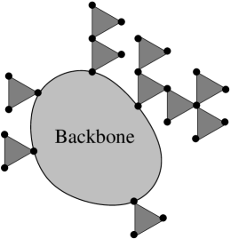
Figure 7: Spins in the backbone (black area) together with some clauses connected to them. The effect of the clauses is $O(\Gamma)$ corrections to effective fields of spins in the backbone.

With the aid of the notation that we just introduced, we will be able to write the resulting expressions in compact form. We focus on the interaction term in the expression for the free energy

$$V=N\gamma\int\left[\Lambda(h_{1},h_{2},h_{3})-\sum_{i=1,2,3}\sqrt{\Gamma^{2}+h_{i}^{2}}\right]\prod_{i=1,2,3}P(h_{i})\mathrm{d}h_{i}$$ (59)

For the remainder of this section when we say $h\approx k$ where $k$ is an integer, we actually mean that $(h-k)/\Gamma=O(1)$.

Let us evaluate the expression in parentheses $\Lambda^{\prime}=\Lambda(h_{1},h_{2},h_{3})-\sum_{i=1,2,3}\sqrt{\Gamma^{2}+h_{i}^{2}}$. Since the expression is symmetric we can assume $h_{1}\leqslant h_{2}\leqslant h_{3}$ without losing generality. To first order in $\Gamma$ the following expressions are obtained for all possible cases:

• $h_{1}<0,|h_{1}|\gg\Gamma$. In this case $\Lambda^{\prime}=0$.

• Neither $h_{1}\approx 0$ nor $h_{1}\approx 1$. Classical expression holds in this case. $\Lambda^{\prime}=-2\min(1,h_{1})$.

• $h_{1}\approx 0\operatorname{and}h_{2}\gg\Gamma$. No degeneracy. Simple answer $\Lambda^{\prime}=-h_{1}-\sqrt{\Gamma^{2}+h_{1}^{2}}$.

• $h_{1}\approx 0,h_{2}\approx 0\operatorname{and}h_{3}\gg\Gamma$. Triple degeneracy. For $\Lambda^{\prime}$ we obtain the following expression:

  $$\Lambda^{\prime}=\Gamma L_{3}(-\tilde{h}_{1},-\tilde{h}_{2})-\Gamma\sum_{i=1,2}\sqrt{1+\tilde{h}_{i}^{2}},$$ (60)

  where $\tilde{h}_{i}=h_{i}/\Gamma$.

• $h_{1}\approx 0,h_{2}\approx 0,h_{3}\approx 0$. 7-fold degeneracy. For $\Lambda^{\prime}$ we have

  $$\Lambda^{\prime}=\Gamma L_{7}(-\tilde{h}_{1},-\tilde{h}_{2},-\tilde{h}_{3})-\Gamma\sum_{i=1,2,3}\sqrt{1+\tilde{h}_{i}^{2}},$$ (61)

  where $\tilde{h}_{i}=h_{i}/\Gamma$.

• $h_{1}\approx 1\operatorname{and}(h_{2}-1)\gg\Gamma$. Double degeneracy. $\Lambda^{\prime}=-2+\Gamma L_{2}(\tilde{h}_{1})-\Gamma\tilde{h}_{1}$.

• $h_{1}\approx 1,h_{2}\approx 1\operatorname{and}(h_{3}-1)\gg\Gamma$. Triple degeneracy.

  $$\Lambda^{\prime}=-2+\Gamma L_{3}(\tilde{h}_{1},\tilde{h}_{2})-\Gamma(\tilde{h}_{1}+\tilde{h}_{2}),$$ (62)

  where $\tilde{h}_{i}=(h_{i}-1)/\Gamma$.

• $h_{1}\approx 1,h_{2}\approx 1,h_{3}\approx 1$. 4-fold degeneracy.

  $$\Lambda^{\prime}=-2+\Gamma L_{4}(\tilde{h}_{1},\tilde{h}_{2},\tilde{h}_{3})-\Gamma(\tilde{h}_{1}+\tilde{h}_{2}+\tilde{h}_{3}),$$ (63)

  where $\tilde{h}_{i}=(h_{i}-1)/\Gamma$.

The self-consistency equation for $P(h)$ can be written in the following form

$$\tilde{P}(\omega)=\exp\frac{\int_{-\infty}^{\infty}\left(\frac{\delta V/N}{\delta P(h)}\right)\mathrm{e}^{i\omega h}\mathrm{d}h}{K(\omega)},$$ (64)

where $K(\omega)=\int\sqrt{\Gamma^{2}+h^{2}}\mathrm{e}^{i\omega h}\mathrm{d}h$. It is convenient to write

$$K(\omega)=-\frac{2}{\omega^{2}}Q(\Gamma\omega),$$ (65)

where $Q(x)$ can be expressed using modified Bessel function of the second kind

$$Q(x)=\frac{|x|}{\sqrt{2\pi}}K_{1}(|x|).$$ (66)

Also observe that $Q(0)=1$. With this replacement we can write

$$\tilde{P}(\omega)=\exp\frac{1}{Q(\omega)}\int_{-\infty}^{\infty}\left[\frac{1}{2}\frac{\mathrm{d}^{2}}{\mathrm{d}h^{2}}\left(\frac{\delta V/N}{\delta P(h)}\right)\right]\mathrm{e}^{i\omega h}\mathrm{d}h.$$ (67)

We seek a solution in the form of a sequence of peaks around integer values of $h$ ($h\approx k$), each peak having a width $O(\Gamma)$. Write

$$P(h)=\frac{1}{\Gamma}\sum_{k=-\infty}^{+\infty}P_{k}\left(\frac{h-k}{\Gamma}\right).$$ (68)

Total probability weight around $h\approx k$ can be expressed as $p_{k}=\int_{-\infty}^{\infty}P_{k}(\tilde{h})\mathrm{d}\tilde{h}$.

The interaction term $V$ has the form proportional to

$$\int\Lambda^{\prime}(h_{1},h_{2},h_{3})P(h_{1})P(h_{2})P(h_{3})\mathrm{d}h_{1}\mathrm{d}h_{2}\mathrm{d}h_{3}.$$ (69)

Computing a variation $\delta V/\delta P(h)$ leaves only two probability distributions in the integral; say $P(h_{2})$ and $P(h_{3})$.

First, we assume that neither $h\approx 0$ nor $h\approx 1$. Note that the two remaining fields in the integrand: $h_{2}$ and $h_{3}$ are necessarily integers. If $h<h_{2},h_{3}$ we know that $\Lambda^{\prime}=\theta(h)\min(1,h)$, which, differentiated twice over $h$ gives just zero.

If $h>h_{2},h_{3}$ and $h-h_{2}\gg\Gamma$, $h-h_{3}\gg\Gamma$, then $\delta V/\delta P(h)$ is actually independent of $h$ and does not survive double differentiation over $h$ either. Note that this holds even if $h\approx 1$ (but either $h_{2}\approx 0$ or $h_{3}\approx 0$).

Therefore, the only non-zero contributions are from $h\approx 0$ and $h\approx 1$. Moreover expressions of the form $\int_{0+\Gamma\infty}^{+\infty}P(h)\mathrm{d}h$ and $\int_{1+\Gamma\infty}^{+\infty}P(h)\mathrm{d}h$ can be replaced with constants $q$ and $q-p_{1}$ ($q=\sum_{k=1}^{+\infty}p_{k}$) since we have seen already that varying with respect to $P(h)$ in these expressions leads to $h$-independent terms.

It is convenient to rewrite $V$ in terms of $P_{k}(\tilde{h})$. We write

$$V/N=2\gamma q^{3}+\gamma\Gamma V^{\prime},$$ (70)

where $V^{\prime}$ takes more complex form

$$V^{\prime} = \int L_{7}(-\tilde{h}_{1},-\tilde{h}_{2},-\tilde{h}_{3})\prod_{i=1,2,3}P_{0}(\tilde{h}_{i})\mathrm{d}\tilde{h}_{i}+3q\int L_{3}(-\tilde{h}_{1},-\tilde{h}_{2})\prod_{i=1,2}P_{0}(\tilde{h}_{i})\mathrm{d}h_{i}$$ (71)

$$+3q^{2}\int\tilde{h}_{1}P_{0}(\tilde{h}_{1})\mathrm{d}\tilde{h}_{1}-3(p_{0}+q)^{2}\int\sqrt{1+\tilde{h}^{2}}P_{0}(\tilde{h})\mathrm{d}\tilde{h}$$

$$+\int L_{4}(\tilde{h}_{1},\tilde{h}_{2},\tilde{h}_{3})\prod_{i=1,2,3}P_{1}(\tilde{h}_{i})\mathrm{d}\tilde{h}_{i}+3(q-p_{1})\int L_{3}(\tilde{h}_{1},\tilde{h}_{2})\prod_{i=1,2}P_{1}(\tilde{h}_{i})\mathrm{d}\tilde{h}_{i}$$

$$+3(q-p_{1})^{2}\int L_{2}(\tilde{h}_{1})P_{1}(\tilde{h}_{1})\mathrm{d}\tilde{h}_{1}-3q^{2}\int\tilde{h}P_{1}(\tilde{h})\mathrm{d}\tilde{h}.$$

We can use the identity $\delta V/\delta P(h)=\delta V/\delta P_{0}(\tilde{h})$ for $h\approx 0$ and $\delta V/\delta P(h)=\delta V/\delta P_{1}(\tilde{h})$ for $h\approx 1$. We have shown that all other terms do not contribute.

For the partial derivatives we obtain the following expression (also taking into account the fact that $P_{0}(\tilde{h})=P_{0}(-\tilde{h})$.

$$\frac{1}{3\gamma\Gamma}\frac{\delta V/N}{\delta P_{0}(\tilde{h})} = \int L_{7}(\tilde{h},\tilde{h}_{2},\tilde{h}_{3})P_{0}(\tilde{h}_{2})P_{0}(\tilde{h}_{3})\mathrm{d}\tilde{h}_{2}\mathrm{d}\tilde{h}_{3}+2q\int L_{3}(\tilde{h},\tilde{h}_{2})P_{0}(\tilde{h}_{2})\mathrm{d}\tilde{h}_{2}$$ (72)

$$+q^{2}\tilde{h}-(p_{0}+q)^{2}L_{2}(\tilde{h})$$

$$\frac{1}{3\gamma\Gamma}\frac{\delta V/N}{\delta P_{1}(\tilde{h})} = \int L_{4}(\tilde{h},\tilde{h}_{2},\tilde{h}_{3})P_{1}(\tilde{h}_{2})P_{1}(\tilde{h}_{3})\mathrm{d}\tilde{h}_{2}\mathrm{d}\tilde{h}_{3}+2(q-p_{1})\int L_{3}(\tilde{h},\tilde{h}_{2})P_{1}(\tilde{h}_{2})\mathrm{d}\tilde{h}_{2}$$ (73)

$$+(q-p_{1})^{2}L_{2}(\tilde{h})-q^{2}\tilde{h}$$

We write the self-consistency equation in the following form

$$\tilde{P}(\omega)=\exp\frac{3\gamma}{Q(\omega)}\left[F_{0}(\Gamma\omega)+\frac{1}{2}\left(\mathrm{e}^{i\omega}F_{1}(\Gamma\omega)+\mathrm{e}^{-i\omega}F_{1}^{\ast}(\Gamma\omega)\right)\right]$$ (74)

where we have denoted

$$F_{0}(\tilde{\omega}) = \int^{\infty}_{-\infty}\left[\frac{1}{2}\frac{\partial^{2}}{\partial\tilde{h}^{2}}\left(\frac{1}{3\gamma\Gamma}\frac{\delta V/N}{\delta P_{0}(\tilde{h})}\right)\right]\mathrm{e}^{-i\tilde{\omega}\tilde{h}}\mathrm{d}\tilde{h},$$ (75)

$$F_{1}(\tilde{\omega}) = \int^{\infty}_{-\infty}\left[\frac{1}{2}\frac{\partial^{2}}{\partial\tilde{h}^{2}}\left(\frac{1}{3\gamma\Gamma}\frac{\delta V/N}{\delta P_{1}(\tilde{h})}\right)\right]\mathrm{e}^{-i\tilde{\omega}\tilde{h}}\mathrm{d}\tilde{h}.$$ (76)

Since for all functions $L_{n}$ we have the identity $\frac{1}{2}\frac{\partial}{\partial\tilde{h}}L(\tilde{h},\ldots)|^{\tilde{h}=+\infty}_{\tilde{h}=-\infty}=1$, we obtain $F_{0}(0)=-q^{2}$ and $F_{1}(0)=q^{2}$.

We now perform the Fourier transform of $\tilde{P}(\omega)$. Since $\tilde{P}(\omega)$ is modulated periodic function with $\omega_{\max}\sim 1/\Gamma$, its Fourier transform is necessarily a series of spikes of width $\Gamma$. This justifies our previous ansatz. Let us compute the probability density for $h\approx k$.

$$P_{k}(\tilde{h})=\int_{-\infty}^{\infty}\mathrm{e}^{ik\omega+i\Gamma\omega\tilde{h}}\exp\frac{3\gamma}{Q(\omega)}\left[F_{0}(\Gamma\omega)+\operatorname{Re}\left\{\mathrm{e}^{i\omega}F_{1}(\Gamma\omega)\right\}\right]\frac{\mathrm{d}\omega}{2\pi}.$$ (77)

Using the smallness of $\Gamma$ and the identity $\int_{-\pi}^{\pi}\mathrm{e}^{a\cos\omega+ik\omega}\frac{\mathrm{d}\omega}{2\pi}=I_{k}(a)$, we can rewrite to leading order in $\Gamma$

$$P_{k}(\tilde{h})=\int^{\infty}_{-\infty}\mathrm{e}^{3\gamma F_{0}(\tilde{\omega})/Q(\tilde{\omega})}I_{k}\left(\frac{3\gamma|F_{1}(\tilde{\omega})|}{Q(\tilde{\omega})}\right)\mathrm{e}^{i\tilde{\omega}\tilde{h}}\frac{\mathrm{d}\tilde{\omega}}{2\pi}.$$ (78)

Note that the integrated probability weights $p_{k}=\int P_{k}(\tilde{h})\mathrm{d}\tilde{h}$ are obtained by substituting $\tilde{\omega}=0$ in the integrand

$$p_{k}=\mathrm{e}^{-3\gamma q^{2}}I_{k}(3\gamma q^{2}).$$ (79)

This is precisely Eq. 18. For $k=0$ using $p_{0}=1-2q$ a self-consistency equation identical to that of $\Gamma=0$, $T=0$ is obtained. Therefore, the value of $q$ is unchanged to leading order in $\Gamma$.

Since $F_{0}(\tilde{\omega})$ and $F_{1}(\tilde{\omega})$ are given solely in terms of $P_{0}(\tilde{h})$ and $P_{1}(\tilde{h})$, $k=0$ and $k=1$ are sufficient to provide a closed system of equations

$$P_{0}(\tilde{h}) = \int^{\infty}_{-\infty}\mathrm{e}^{3\gamma F_{0}(\tilde{\omega})/Q(\tilde{\omega})}I_{0}\left(\frac{3\gamma|F_{1}(\tilde{\omega})|}{Q(\tilde{\omega})}\right)\mathrm{e}^{i\tilde{\omega}\tilde{h}}\frac{\mathrm{d}\tilde{\omega}}{2\pi},$$ (80)

$$P_{1}(\tilde{h}) = \int^{\infty}_{-\infty}\mathrm{e}^{3\gamma F_{0}(\tilde{\omega})/Q(\tilde{\omega})}I_{1}\left(\frac{3\gamma|F_{1}(\tilde{\omega})|}{Q(\tilde{\omega})}\right)\mathrm{e}^{i\tilde{\omega}\tilde{h}}\frac{\mathrm{d}\tilde{\omega}}{2\pi}.$$ (81)

For some critical value of $\gamma$ both trivial ($q=0$) and a non-trivial ($q\neq 0$) solutions coexist. While the appearance of non-trivial $q$ and its value are not sensitive to $\Gamma$ for small values of $\Gamma$, the point where the non-trivial solution becomes stable is.

Also observe that since the integrand is real, all $P_{k}(\tilde{h})$ are symmetric $P_{k}(\tilde{h})=P_{k}(-\tilde{h})$. While this is expected for $P_{0}(\tilde{h})$, such symmetry for $P_{1}(\tilde{h})$ and others is likely only approximate, higher order contributions in $\Gamma$ should make $P_{k}(\tilde{h})\neq P_{k}(-\tilde{h})$ for $k\neq 0$.

Determining the stability of non-trivial solution is accomplished with the aid of Eq. (IV.2). Substituting our ansatz for $P(h)$ we obtain

$$\frac{F}{N}\equiv\frac{F(\Gamma)}{N}=3\gamma q^{2}-4\gamma q^{3}+\sum_{k}|k|p_{k}-2\gamma\Gamma V^{\prime}-\frac{3}{2}\gamma\Gamma V^{\prime\prime}+\Gamma\int\sqrt{1+\tilde{h}^{2}}P_{0}(\tilde{h})\mathrm{d}\tilde{h},$$ (82)

where $V^{\prime}$ has been defined in (71) and $V^{\prime\prime}$ (coming from $\Lambda^{\prime}(+\infty,\ldots)$ term) can be written as

$$V^{\prime\prime} = \int L_{3}(\tilde{h}_{1},\tilde{h}_{2})P_{1}(\tilde{h}_{1})P_{1}(\tilde{h}_{2})\mathrm{d}\tilde{h}_{1}\mathrm{d}\tilde{h}_{2}$$ (83)

$$+ 2(q-p_{1})\int L_{2}(\tilde{h}_{1})P_{1}(\tilde{h}_{1})\mathrm{d}h_{1}-2q\int\tilde{h}P_{1}(\tilde{h})\mathrm{d}\tilde{h}.$$

For $\Gamma=0$ the last three terms disappear and substituting $p_{k}=\mathrm{e}^{-3\gamma q^{2}}I_{k}(3\gamma q^{2})$ we obtain

$$\frac{F(0)}{N}=\gamma q^{2}\left(1-\mathrm{e}^{-3\gamma q^{2}}\left(I_{0}(3\gamma q^{2})+3I_{1}(3\gamma q^{2})\right)\right)$$ (84)

The value of $\gamma=\gamma_{c0}\approx 5.18$ where this expression (with $q\neq 0$ determined from self-consistency equation) becomes positive is the point where non-trivial solution becomes stable. We now calculate the phase transition line $\gamma=\gamma_{c}(\Gamma)$ to the leading order in $\Gamma$ (here $\gamma(0)\equiv\gamma_{c0}$). For $\gamma$ slightly larger than $\gamma_{c0}$, classical expression can be written as

$$\frac{F(0)}{N}=A(\gamma-\gamma_{c}(0)),\qquad A=\left.\frac{\partial F(0,\gamma)}{\partial\gamma}\right|_{\gamma_{c}(0)}\approx 0.0706.$$ (85)

The remaining terms in $F/N$ are linear in $\Gamma$. Write them in the form $-\Gamma\tilde{V}(q)$:

$$\tilde{V}(q) = 2\gamma\int L_{7}(\tilde{h}_{1},\tilde{h}_{2},\tilde{h}_{3})\prod_{i=1,2,3}P_{0}(\tilde{h}_{i})\mathrm{d}h_{i}+6\gamma q\int L_{3}(\tilde{h}_{1},\tilde{h}_{2})\prod_{i=1,2}P_{0}(\tilde{h}_{i})\mathrm{d}\tilde{h}_{i}$$

$$+2\gamma\int L_{4}(\tilde{h}_{1},\tilde{h}_{2},\tilde{h}_{3})\prod_{i=1,2,3}P_{1}(\tilde{h}_{i})\mathrm{d}\tilde{h}_{i}+6\gamma\left(\frac{1}{4}+q-p_{1}\right)\int L_{3}(\tilde{h}_{1},\tilde{h}_{2})\prod_{i=1,2}P_{1}(\tilde{h}_{i})\mathrm{d}\tilde{h}_{i}$$

$$+6\gamma(q-p_{1})\left(\frac{1}{2}+q-p_{1}\right)\int\sqrt{1+\tilde{h}^{2}}P_{1}(\tilde{h})\mathrm{d}\tilde{h}-\left(1+6\gamma(1-q)^{2}\right)\int\sqrt{1+\tilde{h}^{2}}P_{0}(\tilde{h})\mathrm{d}\tilde{h}$$

Let $\tilde{V}_{0}(q_{0})$ denote $\tilde{V}(q)$ computed at $\gamma=\gamma_{c}(0)$ with $P_{0}(\tilde{h})$, $P_{1}(\tilde{h})$ solving self-consistency equation with $q\neq 0$; denote $\tilde{V}_{0}(0)$ similarly computed $\tilde{V}(q)$ at $\gamma=\gamma_{c}$ for trivial solution $q=0$.

To leading order in $\Gamma$, the point $\gamma_{c}$ where nontrivial $q\neq 0$ solution becomes stable is

$$\gamma_{c}(\Gamma)=\gamma_{c}(0)+\Gamma\frac{\tilde{V}_{0}(0)-\widetilde{V_{0}}(q_{0})}{A}.$$ (87)

VI Conclusion

In this paper we have extended the classical treatment of phase transitions in K-SAT ksat1 ; ksat3 ; ksat4 to the quantum domain for the case of $K=3$. Although infinitely-connected quantum spin glass models have been studied, no studies of dilute spin glasses have been performed to the best of our knowledge.

While infinitely-connected models have small ($O(1/\sqrt{N})$ or smaller) couplings, dilute glasses are characterized by strong ($O(1)$) couplings which means that perturbation expansion cannot be truncated. Due to the limitations imposed by the structure of disorder, we have only been able to solve the problem within static approximation using replica symmetric ansatz.

What we have observed is that the quantum limit $\Gamma>0$, $T=0$ is qualitatively similar to the classical limit $\Gamma=0$, $T>0$ (although quantitative results and analytical expressions are quite different). The order parameter in the limit of small $\Gamma$ takes the form of series of peaks of width $O(\Gamma)$, just as in the classical case it takes the form of series of peaks of width $O(T)$. At $\Gamma=0$, $T=0$ we recovet the phase transition at the classical value $\gamma_{c}(0)$. For small but finite $\Gamma$ the value of $\gamma_{c}$ increases linearly, $\gamma_{c}=\gamma_{c}(0)+C\Gamma$, and the expression for the constant $C$ is given in the closed form in terms of the quantities computed at $\Gamma=0$.

Much of the similarities can be explained away by the fact that we ignored dynamic effects. Incorporating the dynamic effects changes the phase diagram of Sherrington-Kirkpatrick model dynamic ; dynamic2 ; dynamic3 . However, static approximation is assumed to work very well in the limit of small $\Gamma$. For the problem at hand this seems to be the only feasible limit. A bigger concern is that we have completely ignored the effects of replica symmetry breaking (RSB). We expect that the location of the dynamic transition for the QAA algorithm should be the same as for simulated annealing, since it is given by $\Gamma=0$, $T=0$. Working in the regime of small $T$ or small $\Gamma$ within RSB will enable us to compare performance of these algorithms for $\gamma\approx\gamma_{d}$.

Another suggestion for future work is K-XOR-SAT problem. It can be solved on a classical computer in polynomial time, but becomes exponentially hard for the simulated annealing algorithm. Owing to simple structure of its energy landscape, many exact results have been obtained for this problem kxorsat . Quantum version of $K$-XOR-SAT in the limit of small $\Gamma$ might be much easier to solve. Note that many of properties of K-SAT are found in K-XOR-SAT, example being a single level of replica symmetry breaking in a certain range of $\gamma$.

We have worked within replica symmetric formalism developed by Monasson monasson that uses a functional order parameter. Alternative method of working with dilute glasses that is closer in spirit to the treatment of SK model has been developed by Viana and Bray vianabray and it incorporates a sequence of various order parameters. The bridge between this approaches have been developed by Kanter and Sompolinsky sompolinsky . A more consistent approach to making static approximation would be to ignore time dependence in a sequence of VB-like order parameters along the lines of qsg1 and convert the result to the form that uses functional order parameter. We have not tried to reconcile that approach with our treatment. It is interesting to see if these approaches are equivalent, and if not, how the answer changes.

Appendix

Matrices ${\cal M}_{j}$ introduced in the Sec. V have the following form:

$${\cal M}_{2}=\left(\begin{array}[]{cc}a&1\\ 1&-a\end{array}\right),$$ (88)

$${\cal M}_{3}=\left(\begin{array}[]{ccc}a+b&1&1\\ 1&a-b&0\\ 1&0&-a+b\end{array}\right),$$ (89)

$${\cal M}_{4}=\left(\begin{array}[]{cccc}a+b+c&1&1&1\\ 1&a+b-c&0&0\\ 1&0&a-b+c&0\\ 1&0&0&-a+b+c\end{array}\right),$$ (90)

$${\cal M}_{7}=\left(\begin{array}[]{ccccccc}a+b+c&1&1&0&1&0&0\\ 1&a+b-c&0&1&0&1&0\\ 1&0&a-b+c&1&0&0&1\\ 0&1&1&a-b-c&0&0&0\\ 1&0&0&0&-a+b+c&1&1\\ 0&1&0&0&1&-a+b-c&0\\ 0&0&1&0&1&0&-a-b+c\end{array}\right).$$ (91)

References

• (1) S. Cook, “The complexity of theorem-proving procedures”, Proc. 3rd Ann. ACM Symposium on Theory of Computing, p.151 (1971).
• (2) P. Shor, “Algorithms for quantum computation: Discrete logarithms and factoring” , Proc. 35th Ann. Symp. on Foundations of Computer Science, p.124 (1994).
• (3) E. Farhi, J. Goldstone, S. Gutmann, M. Sipser, “Quantum Computation by Adiabatic Evolution”, arXiv:quant-ph/0001106.
• (4) E. Farhi, J. Goldstone, S. Gutmann, J. Lapan, A. Lundgren, and D. Preda, Science 292, 472 (2001).
• (5) W. Van Dam, M. Mosca, U. Vazirani, ”How Powerful is adiabatic Quantum Computation?”, arXiv:quant-ph/0206003.
• (6) E. Farhi, J. Goldstone, S. Gutmann, “Quantum Adiabatic Evolution Algorithms versus Simulated Annealing”, arXiv:quant-ph/0201031.
• (7) V. N. Smelyanskiy, S. Knysh, and R. D. Morris Phys. Rev. E 70, 036702 (2004).
• (8) A.J. Bray, M.A. Moore, “Replica theory of quantum spin glasses”, J. Phys. C 13, L655 (1980).
• (9) T. Yamamoto and H. Ishii, “A perturbation expansion for the Sherrington-Kirkpatrick model with a transverse field”, J. Phys. C 20, p.6053 (1987).
• (10) K.D. Usadel and B. Schmitz, “Quantum fluctuations in an ising spin glass with transverse field”, Solid State Comm., 64, p.975 (1987).
• (11) T.K. Kopec, “A dynamic theory of transverse freezing in the Sherrington-Kirkpatrick Ising model”, J. Phys. C 21 p.6053 (1988)
• (12) D.S. Fisher, “Critical behavior of random transverse-field Ising spin chains.”, Phys. Rev. B 51, 6411 (1995).
• (13) B.W. Reichardt, “The quantum adiabatic optimization algorithm and local minima”, Proceedings of the 36 annual ACM symposium on Theory of computing, pp. 502-510 (Chicago, IL, USA, 2004).
• (14) S. Knysh, V.N. Smelyanskiy, “Adiabatic Quantum Computing in systems with constant inter-qubit couplings”, arXiv:quant-ph/0511131.
• (15) P. Cheeseman, B. Kanefsky, W.M. Taylor, “Where the REALLY Hard Problems Are”, Proc. 12th Int. Joint Conf. Artificial Intelligence, p.331 (1991).
• (16) S. Finch, “Mathematical Constants”, Encyclopedia of Mathematics and its Applications 94, Cambridge University Press (2003).
• (17) P. Erdos, A. Renyi, “On the evolution of random graphs”, Publ. Math. Inst. Hung. Acad. Sci. (1960).
• (18) R. Monasson, R. Zecchina, S. Kirkpatrick, B. Selman and L. Troyansky, “Determining computational complexity from characteristic ’phase transitions”’, Nature 400, p.133 (1999).
• (19) M. Mezard, G. Parisi, R. Zecchina, “Analytic and Algorithmic Solution of Random Satisfiability Problems”, Science 297, p.812 (2002).
• (20) R. Monasson, R. Zecchina, “Statistical mechanics of the random K-satisfiability problem”, Phys. Rev. E 56, p.1357 (1997).
• (21) R. Monasson, R. Zecchina, “Entropy of the K-Satisfiability Problem”, Phys. Rev. Lett. 76, p.3881 (1996).
• (22) M. Mezard, R. Zecchina, “The random K-satisfiability problem: from an analytic solution to an efficient algorithm”, Phys. Rev. E 66, 056126 (2002).
• (23) M. Mezard, G. Parisi, M.A. Virasoro, “Spin Glass Theory and Beyond”, World Scientific, Singapore (1987).
• (24) P.M. Duxbury, “Percolation of frozen order in glassy combinatorial problems”, arXiv:cond-mat/0308211.
• (25) M. Mezard, F. Ricci-Tersenghi, R. Zecchina, “Alternative solutions to diluted p-spin models and XORSAT problems”, J. Stat. Phys. 111, p.505 (2003).
• (26) R. Monasson, “Optimization problems and replica symmetry breaking in finite connectivity spin glasses”, J. Phys. A 31, p.513 (1998).
• (27) L. Viana and A.J. Bray, “Phase diagrams for dilute spin glasses”, J. Phys. C 18 p.3037 (1985).
• (28) I. Kanter, H. Sompolinsky, “Mean-field theory of spin-glasses with finite coordination number”, Phys. Rev. Lett. 58, p.164 (1987).