Nuclear Spin Noise and STM Noise Spectroscopy

Abstract

We consider fluctuations of the electronic spin due to coupling to nuclear spin. Noise spectroscopy of an electronic spin can be revealed in the Scanning Tunnelling Microscope (STM). We argue that the noise spectroscopy of electronic spin can reveal the nuclear spin dynamics due to hyperfine coupling. Tunnelling current develops satellites of the main lines at Larmor frequency and at zero frequency due to hyperfine coupling. We also address the role of the rf field that is at or near the resonance with the nuclear hyperfine field. This approach is similar to Electron Nuclear Double Resonance (ENDOR), in that is allows one to detect nuclear spin dynamics indirectly through its effect on electronic spin.

I Introduction

Noise spectroscopy is a technique that allows one to measure spectroscopic properties by observing nontrivial features in the noise. The main feature of noise spectroscopy is that the noise spectrum has encoded in it spectroscopic features that correspond to physical excitations in the system, such as atomic levels, Zeeman split levels of electrons or nuclear levels. The transition between levels would cause enhanced dissipation when the energy transferred equals the energy difference between those levels. This enhanced dissipation also would imply enhanced fluctuations at the same frequencies/energies, as follows from the fluctuation-dissipation theorem. Experiments that prove utility of the noise are available from many fields. An incomplete list includes nuclear spin noise,Sleater85 Faraday rotation noise in the alkali atoms,Aleksandrov81 ; Mitsui01 ; Crooker04 and acoustic noise.Lobkis01 Recently noise spectroscopy was used to detect a single electronic spin with Magnetic Resonance Force Microscopy by an IBM group.Rugar04

Therefore, in principle, noise measurement could be a powerful tool to investigate the dynamics of the system. Sometimes noise is easier to measure and then noise spectroscopy could be even a preferred technique to investigate nano-scale systems.Rugar04 ; Crooker04

One example of the noise spectroscopy relevant for us here is Electronic Spin Resonance Scanning Tunneling Microscopy, ESR-STM. ESR-STM is a technique that is using the extremely local nature of the STM measurement to detect the noisy precession of spin centers on the nonmagnetic surface. When a tip of an STM is located above a paramagnetic spin center the tunneling current is modulated by the precession in the presence of external field. It was shown22 ; 23 that the ac current at the Larmor frequency is spatially localized within $0.5-1nm$. It is the spatial localization that suggests that this technique is capable of detecting a single spin. In addition it was proved that the frequency of the signal is dependent on real time on the size of the magnetic field.24 ; 25 More recently similar experiments have been done on the paramagnetic BDPA molecule.26 The interest in this technique has risen sharply recently, due to the possibility to manipulate and detect a single spin27 ; 33 and due to the possibility to use it for quantum computation.27 ; 28 There have been many proposals for the mechanism of this phenomenon.29 ; 30 ; 32 ; 33 ; 34 ; 35 ; 36 Present experiments are not sufficient to constraint possible mechanism and further investigation would help to elucidate the nature of the effect.

Recently Durkan reported the measurements of the noise in the ESR-STM on a TEMPO molecule.Durkan04 This molecule is well characterized, and it contains nitrogen $N$ with the nuclear spin $I=1$. ESR spectrum of TEMPO in the bulk is known to exhibit the hyperfine splitting on the order of   15 G that corresponds to the free ($g_{e}=2$) electron precession frequency on the order of 45 Mhz. The main new observation that is important in our context is that the ESR-STM on TEMPO molecule produced three peaks that possibly corresponds to the hyperfine split Larmor line in current spectrum. If reproduced, this observation opens up a new possibilities in noise spectroscopy in STM.

The purpose of this paper is to consider the case of coupling of the electronic impurity spin $S$ to nuclear spin $I$ via hyperfine coupling. We investigate the noise spectroscopy of the nuclear spin and coupled electron-nuclear dynamics as it might be seen in STM experiments. Indeed all the previous discussions of the mechanisms so far have focused on the dynamics of the electronic impurity spin. Hyperfine coupling to the nuclear spin would allow one to measure dynamics, relaxation times and transitions between the nuclear levels.

We find that the hyperfine coupling produces additional satellite lines in the noise spectra for the localized impurity spin that will be split away from Larmor line by the amount proportional to hyperfine coupling $A$. We also consider the case of the rf field at frequency $\omega\sim A$ applied to the system. This is the case of Electronic-Nuclead Double Resonance (ENDOR), where electron spin dynamics will be affected by the nuclear spin flips caused by the rf field. In the case of applied rf field we clearly pump energy into the system and hence measurement is not strictly a noise spectroscopy measurement. Still this is a set up most likely to be attempted experimentally and this is why we address it here as well.

The plan of the paper is as follows. We address the localized impurity spin susceptibility with the hyperfine coupling and the tunneling current modulations in the Sec.II. We address a few specific cases, such as case of no rf field and case of no applied fields, neither dc nor ac. In all of these cases electronic spin will have nontrivial spectroscopic features, most notable the hyperfine split lines around Larmor line and around zero frequency. In Sec III we conclude with discussion of possible experiments.

II Probing the spin susceptibility via noise measurement

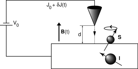
Figure 1: Sketch of the experimental setup. The tip — surface separation distance is $d$. The single magnetic impurity atom with spin ${\bf S}$ on the substrate surface interacts with the nuclear spin ${\bf I}$ in the substrate.

To be specific, consider the tunneling current between two contacts in the presence of a localised spin ${\bf S}$ interacting with a nuclear spin ${\bf I},\ I=1$, to make a contact with the experiments on TEMPO. The Hamiltonian of this system is written in the form

$${\cal H}={\cal H}_{L}+{\cal H}_{R}+{\cal H}_{S}+\sum_{kp\alpha\beta}c_{k\alpha}^{\dagger}[t_{0}+t_{1}{\bf S}\cdot\sigma_{\alpha\beta}]c_{p\beta},$$ (1)

where ${\cal H}_{L(R)}=\sum_{k(p)\sigma}\varepsilon_{k(p)\sigma}c_{k(p)\sigma}^{\dagger}c_{k(p)\sigma}$ models free electrons in the left (right), $L(R)$, lead, whereas

$${\cal H}_{S} = B_{0}S^{z}+A{\bf S}\cdot{\bf I}+B_{1}I^{x}\cos{\omega t}+B_{2}S^{x}\cos{\omega t},$$

$$B_{0}\gg A\gg B_{1},B_{2}$$

accounts for the interactions between the localised electronic and nuclear spins. In the Hamiltonian, Eq. (1), $\sigma_{\alpha\beta}$ denote the Pauli spin matrix vector with matrix indices $\alpha,\beta$, the Fermionic $c_{k(p)\sigma}^{\dagger},c_{k(p)\sigma}$ are creation and annihilation operators of electrons in the $k$th ($p$th) eigenstate in the STM tip (substrate surface), with spin $\sigma=\uparrow,\downarrow$. For simplicity we have incorporated the electronic $g_{e}$ and nuclear gyromagnetic ratio $g_{N}$ into the effective fields $B_{0}=g_{e}H_{0},\ B_{1}=g_{N}H_{1},B_{2}=g_{e}H_{1}$ for the external dc field $H_{0}$ and ac field $H_{1}\cos\omega t$.

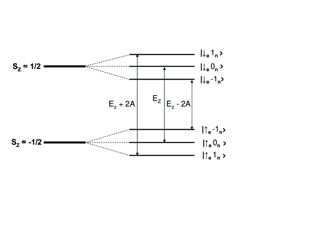
Figure 2: The possible spin-flip transitions that may occur in the system. The electronic spin-flips give rise to the three major peaks in the transport current fluctuations spectrum at the frequencies $E_{z}$ and $E_{z}\pm 2A$; see also Fig. 3 and Fig. 4.

The last term in Eq. (1) describes tunneling of the electrons from the tip into the substrate surface in the presence of the localised electronic spin ${\bf S}$. This term only give a contribution to the net steady state current by providing a chemical potential shift (bias voltage drop) between the two bands $\{\varepsilon_{k\sigma}\}$ and $\{\varepsilon_{p\sigma}\}$. In real systems, the hopping matrix elements $\hat{t}=t_{0}+t_{1}{\bf S}\cdot\sigma$ have a $kp-$ dependence, which are omitted here in order to make the notation more compact. The wavefunctions of our system are superpositions of the direct product states $|\psi_{L}\rangle\otimes|\psi_{S}\rangle\otimes|\psi_{R}\rangle$, e.g. the direct product of the state of the STM tip, the impurity spin, and the substrate surface. The tunneling matrix $\hat{t}$ in the last term of Eq. (1) couples all of these different states, of which the term proportional to $t_{0}$ describes the spin independent tunneling while the term proportional to $t_{1}$ provides the spin dependent contributions arising from the exchange interaction of tunneling electrons to the magnetic atom.

Spin dependence of the tunneling arise due to direct exchange dependence of the tunnel barrier.balatsky2002 The overlap of the electronic wavefunctions of the tip and the surface, separated by a disctance $d$ is exponentially small and is given by a spin dependent tunneling matrix element $\hat{t}=\gamma\exp\{-\sqrt{(\Phi-J{\bf S}(t)\cdot\sigma)/\Phi_{0}}\}$, where the direct exchange between the tunneling electron spin $\sigma$ and the impurity spin ${\bf S}$ is explicitly included. Here, $J$ is the exchange interaction parameter between the electrons tunneling from the tip to the surface and the precessing impurity spin ${\bf S}$. The tunneling barrier height $\Phi$ is typically a few eV, whereas $\Phi_{0}=\hbar^{2}/(8md^{2})$ is related to the distance between the tip and the surface.tersoff1993 Since the exchange term in the exponent is small compared to the barrier height, we may expand the exponent in $JS$, which gives $\hat{t}=t_{0}+t_{1}{\bf S}(t)\cdot\sigma$. Here, $t_{0}=\gamma\exp{(-\sqrt{\Phi/\Phi_{0}})}\cosh{[JS/(2\sqrt{\Phi\Phi_{0}})]}$ describes the spin independent tunneling, while $t_{1}=\gamma\exp{(-\sqrt{\Phi/\Phi_{0}})}\sinh{[JS/(2\sqrt{\Phi\Phi_{0}})]}$ accounts for the spin dependent tunneling amplitude. For estimates we may employ the typical thumb rule $t_{1}/t_{0}\approx JS/(2\Phi)\ll 1$.

We will assume that the tunneling electrons are partially spin polarised. This can be achieved in several situations. For example, in ferromagnetically coated tips a potential difference $2\delta\mu_{\sigma}$ separates the spin bands $\varepsilon_{k\sigma}=\varepsilon_{k}+\sigma\delta\mu_{\sigma}$. Ferromagntically ordered tips have proven successful in the study of magnetic structures.fmtips Another approach to obtain a spin polarised current is to use an antiferromagntically coated tip with no ferromagnetic order.afmtips Such tips have the benefit of a vanishing dipolar field and should, therefore, have a negligible influence on the precession frequency of the impurity spin. A ferromagnetically ordered tip may produce a field of ${\cal O}(1)$ T at a separation of few Ångströms from the surface. Such fields therefore leads to huge precession frequencies which are difficult to measure. In what follows, however, we will not be concerned of how the spin polarised current is generated. We define a parameter ${\cal A}$ which relates the spin polarised current to the net tunneling current. This is the parameter that will be determined by a particular microscopic model of the tip. Thus, we will henceforth treat ${\cal A}$ as a phenomenological parameter.

For conciseness, we employ the Heisenberg picture for all operators $\{O\}$, i.e. $O(t)=\exp{[iHt]}O_{S}\exp{[-iHt]}$, with $O_{S}=O(t)$ for operators in the Schrödinger picture. All finite temperature expectation values $\langle{O(t)}\rangle$ will represent $\sum_{i}p_{i}\langle\psi_{i}(0)|O(t)|\psi_{i}(0)\rangle$, where $\psi_{i}(t=0)$ is the zero time wave function from the Schrödinger picture, whereas $p_{i}$ is its probability within the density matrix formulation.

Now, for a qualitative description of the effect addressed here consider the charge current $J(t)=-e\partial/\partial tN_{L}(t)$. Since we are considering the steady state regime it is, by charge and current conservation, sufficient to consider the current in the tip (or in the substrate) only. By a direct calculation, using the Heisenberg equation of motion, we find that

$$J(t)=-2e{\rm Im}\sum_{kp\alpha\beta}\Bigl{\langle}c_{k\alpha}^{\dagger}[t_{0}+t_{1}{\bf S}(t)\cdot\sigma_{\alpha\beta}]c_{p\beta}\Bigr{\rangle},$$ (3)

where $e$ is the electronic charge. Hence, we see that the tunneling current can be partitioned into a spin independent part $J_{0}(t)=-2e{\rm Im}\sum_{kp\sigma}t_{0}\langle{c_{k\sigma}^{\dagger}c_{p\sigma}}\rangle$ and a spin dependent part

$$\delta J(t)=\langle{\delta{\bf J}(t)}\rangle=et_{1}\langle{{\bf S}(t)\cdot{\bf J}_{s}(t)}\rangle,$$ (4)

which depends on the localised moment ${\bf S}(t)$, where

$${\bf J}_{s}(t)=-i\sum_{kp\alpha\beta}c_{k\alpha}^{\dagger}\sigma_{\alpha\beta}c_{p\beta}+H.c.,$$ (5)

is the spin dependent contribution to the tunneling current. The $z$-component of this expression, e.g. $J^{z}_{s}(t)=-i\sum_{kp}(c_{k\uparrow}^{\dagger}c_{p\uparrow}-c_{k\downarrow}^{\dagger}c_{p\downarrow})+H.c.$, describes the net flow of spin $\uparrow$ and spin $\downarrow$ carriers, whereas the transversal component $(J^{x}_{s},J^{y}_{s})(t)=-i\sum_{kp}(c_{k\uparrow}^{\dagger}c_{p\downarrow}+c_{k\downarrow}^{\dagger}c_{p\uparrow},-ic_{k\uparrow}^{\dagger}c_{p\downarrow}+ic_{k\downarrow}^{\dagger}c_{p\uparrow})+H.c.$ accounts for spin flip transitions of the tunneling electrons caused by the interactions with the precessing impurity spin.

To the lowest order in the tunneling amplitude $t_{1}$, the electronic current-current correlation function arising due to the spin dependent part of the current is given by

$$\langle{\{{\delta{\bf J}(t)},{\delta{\bf J}(t^{\prime})}\}}\rangle=(et_{1})^{2}\langle{S^{i}(t)S^{j}(t^{\prime})}\rangle\langle{J_{s}^{i}(t)J_{s}^{j}(t^{\prime})}\rangle$$

$$+(t\leftrightarrow t^{\prime}),$$ (6)

where $\langle{\{{\cdot},{\cdot}\}}\rangle$ denotes the symmetrized correlator whereas $i,j=x,y,z$ signify the spin components. Thus, to lowest non-trivial order in $t_{1}$ we can treat the two temporal correlation functions $K^{ij}(t-t^{\prime})=\langle{S^{i}(t)S^{j}(t^{\prime})}\rangle$ and $C(t-t^{\prime})=\langle{J_{s}^{i}(t)J_{s}^{j}(t^{\prime})}\rangle\rightarrow\langle{J_{s}^{i}(t)}\rangle\langle{J_{s}^{j}(t^{\prime})}\rangle,\ (|t-t^{\prime}|\rightarrow\infty)$ independently. To make a connection with the main proposal of this paper we note that the Fourier transform of the symmetrized correlation function $\langle{\{{\delta{\bf J}(t)},{\delta{\bf J}(t^{\prime})}\}}\rangle$ is the current noise spectrum at various frequencies arising from the localised electronic spin. In Fourier space, the current noise spectrum is given by the convolution of the two power spectra associated with ${\bf S}$ and $\sigma$, e.g.

$$\langle{|\delta{\bf J}(\varepsilon)|^{2}}\rangle=\frac{(et_{1})^{2}}{2\pi}\int K^{ij}(\varepsilon^{\prime})C(\varepsilon-\varepsilon^{\prime})d\varepsilon^{\prime}+(\varepsilon\rightarrow-\varepsilon).$$ (7)

In order to see the effect of the interactions between the localised electronic (${\bf S}$) and nuclear (${\bf I}$) spin in the rotating magnetic field we have to calculate $K^{+-}(\varepsilon)$ and $K^{z}(\varepsilon)$, for which the details are given in the appendix, see Eqs. (18) and (20). The resulting expressions for the correlation functions are given by

$$K^{+-}(\tau) \sim \biggl{(}\frac{1}{4}\biggl{[}1+2\Bigl{(}\frac{B_{1}}{2\omega_{1}}\Bigr{)}^{2}\biggl{(}1+\Bigl{(}\frac{B_{1}}{2\omega_{1}}\Bigr{)}^{2}\biggr{)}+5\Bigl{(}\frac{\Delta\omega}{\omega_{1}}\Bigr{)}^{4}\biggr{]}+\frac{1}{4}\Bigl{(}\frac{B_{1}}{2\omega_{1}}\Bigr{)}^{2}\biggl{(}3-\Bigl{(}\frac{\Delta\omega}{\omega_{1}}\Bigr{)}^{2}\biggr{)}\cos\omega\tau+\frac{3}{4}\Bigl{(}\frac{B_{1}}{2\omega_{1}}\Bigr{)}\cos 2\omega_{1}\tau$$ (8)

$$+\frac{1}{8}\biggl{(}1+\frac{\Delta\omega}{\omega_{1}}\biggr{)}^{4}\cos(\omega+2\omega_{1})\tau+\frac{1}{8}\biggl{(}1-\frac{\Delta\omega}{\omega_{1}}\biggr{)}^{4}\cos(\omega-2\omega_{1})\tau$$

$$+\Bigl{(}\frac{B_{1}}{2\omega_{1}}\Bigr{)}^{2}\biggl{(}1-3\Bigl{(}\frac{\Delta\omega}{\omega_{1}}\Bigr{)}^{2}\biggr{)}[\cos\frac{\omega\tau}{2}-\cos\omega_{1}\tau]$$

$$+2\frac{\Delta\omega}{\omega_{1}}\Bigl{(}\frac{B_{1}}{2\omega_{1}}\Bigr{)}^{2}\biggl{(}1+\frac{\Delta\omega}{\omega_{1}}\biggr{)}\cos\frac{\omega+2\omega_{1}}{2}\tau-2\frac{\Delta\omega}{\omega_{1}}\Bigl{(}\frac{B_{1}}{2\omega_{1}}\Bigr{)}^{2}\biggl{(}1-\frac{\Delta\omega}{\omega_{1}}\biggr{)}\cos\frac{\omega-2\omega_{1}}{2}\tau$$

$$+\frac{1}{2}\Bigl{(}\frac{B_{1}}{2\omega_{1}}\Bigr{)}^{2}\biggl{(}1+\frac{\Delta\omega}{\omega_{1}}\biggr{)}^{2}\cos(\omega+\omega_{1})\tau+\frac{1}{2}\Bigl{(}\frac{B_{1}}{2\omega_{1}}\Bigr{)}^{2}\biggl{(}1-\frac{\Delta\omega}{\omega_{1}}\biggr{)}^{2}\cos(\omega-\omega_{1})\tau$$

$$-\frac{1}{2}\Bigl{(}\frac{B_{1}}{2\omega_{1}}\Bigr{)}^{2}\biggl{(}1+\frac{\Delta\omega}{\omega_{1}}\Bigr{)}^{2}\cos\frac{\omega+4\omega_{1}}{2}\tau-\frac{1}{2}\Bigl{(}\frac{B_{1}}{2\omega_{1}}\Bigr{)}^{2}\biggl{(}1-\frac{\Delta\omega}{\omega_{1}}\Bigr{)}^{2}\cos\frac{\omega-4\omega_{1}}{2}\tau\biggr{)}e^{-i2B_{0}\tau}.$$

and

$$K^{z}(\tau) \sim \frac{1}{4}\Biggl{[}\biggl{(}1+\Bigl{(}\frac{\Delta\omega}{\omega_{1}}\Bigr{)}^{2}\biggr{)}\biggl{(}1+5\Bigl{(}\frac{\Delta\omega}{\omega_{1}}\Bigr{)}^{2}\biggr{)}+4\Bigl{(}\frac{B_{1}}{2\omega_{1}}\Bigr{)}^{4}\Biggr{]}+\frac{3}{4}\Bigl{(}\frac{B_{1}}{2\omega_{1}}\Bigr{)}^{4}[\cos\omega\tau+\cos 2\omega_{1}\tau]$$ (9)

$$+\frac{1}{8}\biggl{(}1+\frac{\Delta\omega}{\omega_{1}}\biggr{)}\biggl{(}\Bigl{[}1-\frac{\Delta\omega}{\omega_{1}}\Bigr{]}^{2}-2\Bigl{(}\frac{\Delta\omega}{\omega_{1}}\Bigr{)}^{2}\biggr{)}\cos(\omega+2\omega_{1})\tau$$

$$+\frac{1}{8}\biggl{(}1-\frac{\Delta\omega}{\omega_{1}}\biggr{)}\biggl{(}\Bigl{[}1+\frac{\Delta\omega}{\omega_{1}}\Bigr{]}^{2}-2\Bigl{(}\frac{\Delta\omega}{\omega_{1}}\Bigr{)}^{2}\biggr{)}\cos(\omega-2\omega_{1})\tau$$

$$+\Bigl{(}\frac{B_{1}}{2\omega_{1}}\Bigr{)}^{2}\biggl{(}1+3\Bigl{(}\frac{\Delta\omega}{\omega_{1}}\Bigr{)}^{2}\biggr{)}[\cos\frac{\omega\tau}{2}+\cos\omega_{1}\tau]-2\Bigl{(}\frac{\Delta\omega}{\omega_{1}}\Bigr{)}^{2}\Bigl{(}\frac{B_{1}}{2\omega_{1}}\Bigr{)}^{2}[\cos\frac{\omega+2\omega_{1}}{2}\tau+\cos\frac{\omega-2\omega_{1}}{2}\tau]$$

$$-\frac{1}{2}\Bigl{(}\frac{B_{1}}{2\omega_{1}}\Bigr{)}^{4}[\cos(\omega+\omega_{1})\tau+\cos(\omega-\omega_{1})\tau+\cos\frac{\omega+4\omega_{1}}{2}\tau+\cos\frac{\omega-4\omega_{1}}{2}\tau]$$

In the above equations we have defined the detuning parameter $\Delta\omega=A-\omega/2$ and the parameter $\omega_{1}=\sqrt{\Delta\omega^{2}+(B_{1}/2)^{2}}$. Resonant conditions of the system is given for $\Delta\omega=0\ \Leftrightarrow\ \omega=2A$ giving $\omega_{1}=B_{1}/2$. While the coefficients $(B_{1}/2\omega_{1})^{2n}\ n=1,2$, rapidly decays to zero out of resonance, the coefficients $(\Delta\omega/\omega_{1})^{2n},\ n=1,2$, rapidly grows to unity, since the amplitude of the rf field $B_{1}\ll A$. Hence, all terms in Eqs. (8) and (9), but the ones proportional to $\cos(\omega\pm 2\omega_{1})\tau/2$, contribute to the spectrum at resonance, whereas only the peaks at $\varepsilon=2B_{0}$ and $\varepsilon=2B_{0}\pm(\omega\pm 2\omega)$ give a non-negligible contribution to the spectrum out of resonance. Below we will focus on few experimentally relevant possibilities.

II.0.1 $B_{0}\neq 0,\ B_{1}\neq 0$

This case corresponds to applying an external DC field and rf field in or close to nuclear resonance, which is known as Electronic Nuclear double Resonance (ENDOR).Slichter Under those circumstances the nuclear spin dynamics is influenced by the rf field, which is reflected in the dynamics of the electonic spin. This is perhaps one of the most relevant cases for nuclear spin noise to be seen in STM experiments.

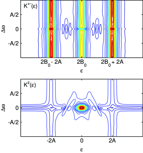
Figure 3: Contour plots of the spectral intensities $K^{+-}(\epsilon)$ (upper panel) and $K^{z}(\varepsilon)$ (lower panel) as function of the detuning $\Delta\omega$ in Fourier space ($\varepsilon$). The spectra are generated by Lorentzian functions of uniform width $\Gamma/B_{0}=1/60$, using $A/B_{0}=1/12$ and $B_{1}/B_{0}=1/100$.

Clearly, the correlation function $K^{+-}$ in Eq. (8) has a central peak at the Larmor frequency $\varepsilon=2B_{0}$, which at resonance is represented by the first, third and seventh terms in Eq. (8). This peak should also be measurable out of resonance since the constant (first) term is non-vanishing for all frequencies of the rf field. There are side-bands around the frequency $\varepsilon=2B_{0}\pm 2A$, represented by the second, third, fourth, tenth, and eleventh terms, of which only the fourth and fifth are present out of resonance. Hence, also these peaks should be seen for all rf frequencies. However, at resonant conditions there are peaks around $\varepsilon=2B_{0}\pm A$, represented by the sixth, eighth, ninth, twelfth, and thirteenth terms in Eq. (8), which are not expected to be measurable appreciably far out of resonance. The same observations hold for the correlation function $K^{z}$, although its spectrum is centred around $\varepsilon=0$. Hence, the central peak of this part is hidden in the white noise spectrum.

In Fig. 3 we display a contour plot of the correlation functions $K^{+-}$ (upper panel) and $K^{z}$ (lower panel) as function of the Fourier frequency $\varepsilon$ and detuning $\Delta\omega$. Especially for $K^{+-}$ it is readily seen that there are five peaks ($2B_{0},\ 2B_{0}\pm A,\ 2B_{0}\pm 2A$) around resonant conditions $\Delta\omega=0$, while only three peaks remain out of resonance. In Fig. 4 (solid) we show that total spectrum at resonance for the same conditions as in Fig. 3.

II.0.2 $B_{0}\neq 0,\ B_{1}=0$

The second case we consider is the case of a nuclear spin noise in a nondriven limit: $B_{0}\neq 0,\ B_{1}=0\ (\omega=0)$. In this case the nuclear hyperfine field provides a flustuating field sampled by the electronic spin. Thus the total field will be given by a sum of the external field, $B_{0}$, and the $AI_{z}$ term. In this case the Larmor line will acquire sidebands due to the nuclear hyperfine field. This is clearly seen from Eq. (8), which in the present case reduces to

$$K^{+-}(\tau)\sim\frac{5}{4}(1+8\cos 2A\tau)e^{-i2B_{0}\tau},$$ (10)

since $\omega_{1}=|\Delta\omega|=A$ giving $\Delta\omega/\omega_{1}=1$. Obviously, this expression provides a main peak at $\varepsilon=2B_{0}$ and sidebands at $\varepsilon=2B_{0}\pm 2A$, as is illustrated in Fig. 4 (dotted). Similarly, the $z$-component of the spin-spin correlation function reduces to

$$K^{z}(\tau)\sim 3-2\cos 2A\tau.$$ (11)

Thus, there are dips at $\varepsilon=\pm 2A$, as seen in Fig. 4. Note that the amplitude of both $K^{+-}$ and $K^{z}$ are independent of the nuclear hyperfine field in this case, however the positions of the peaks obviously shift linearly with $A$.

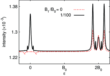
Figure 4: Intensity of the normalised $K^{+-}(\varepsilon)+K^{z}(\varepsilon)$ with (solid) and without (dotted) rf field applied over the system.

Finally we comment on the case with no external field, e.g. $B_{0},B_{1}=0$. Then, the impurity spin interact with the nuclear spin via the nuclear hyperfine field $A$. Assuming that the nuclear spin has a a very slow time dependent dynamics we can use the theory developed in the former section. Thus, under these circumstances the spin-spin correlation functions will reduce to

$$K^{+-}(\tau)\sim\frac{5}{4}(1+8\cos 2A\tau),$$ (12a)

$$K^{z}(\tau)\sim 3-2\cos 2A\tau.$$ (12b)

As expected, the $z$-component of the correlation function is unaffected by the absence of the field $H_{0}$, whereas the transverse component is translated to $\varepsilon_{0}=0$ as $B_{0}\rightarrow 0$. Hence, the spectrum for $K^{z}$ is the same as in Fig. 4 (dotted), as well as the spectrum for $K^{+-}$, however, shifted to $\varepsilon=0$.

III Conclusion

In conclusion we presented a theory for nuclear spin noise spectroscopy. We considered a specific case of an ESR STM where the nuclear spin dynamics is revealed in the tunnelling current noise. We argue that noise spectroscopy is capable of detecting nuclear spin fluctuation via a hyperfine coupling to localized impurity electronic spin. We find that the spectrum of the noise is rich and depends sensitively on the rf frequency and detuning, Fig. 3. The main features of the spectrum are i) the peak at the Larmor electronic frequency that acquires hyperfine split satellites. This part of the spectrum is coming from the transverse spin fluctuations. The ENDOR like phenomenon occurs in the noise spectrum where the nuclear spin flips due to the rf field with nuclear resonance frequency directly affect the electronic spin dynamics. ii) the peak at zero frequency (that realistically will always be obscured by the $1/f$ noise) also acquires satellites at $\pm A$. This observation suggests that one measure the nuclear spin dynamics even in the absence of external fields. as long as the hyperfine lines are outside the $1/f$ noise peak.

Appendix A Derivation of the spin susceptibility

In the paper we have been considering the interaction between an impurity spin ${\bf S}\ (S=1/2)$ on the substrate surface and a nuclear spin ${\bf I}\ (I=1)$ in the substrate. The spin Hamiltonian for this system can be written as

$${\cal H}_{S}=B_{0}S_{z}+AS\cdot I+B_{1}I_{x}\cos{\omega t}+B_{2}S_{z}\cos{\omega t},$$ (13)

with $B_{0}\gg A\gg B_{1},B_{2}$, which yields the effective Hamiltonian

$${\cal H}^{\text{eff}}_{S}=B_{0}S_{z}+AS_{z}I_{z}+B_{1}I_{x}\cos{\omega t}.$$ (14)

A.1 $K^{+-}$

In order to see the effect of the electron spin flips on the susceptibility, we consider the correlation function $K^{+-}(t_{1},t_{2})={\rm tr}\;\{S_{+}(t_{1})S(t_{2})\rho\}$, where $S_{\pm}(t_{1})=\exp\{i\int_{0}^{t_{1}}{\cal H}^{\text{eff}}_{S}dt\}S_{\pm}\exp\{-i\int_{0}^{t_{1}}{\cal H}^{\text{eff}}_{S}dt\}$, $S_{+}=|\uparrow\rangle_{e}\langle\downarrow|$, $S_{-}=|\downarrow\rangle_{e}\langle\uparrow|$, and $\rho=(|\uparrow\rangle_{e}\langle\uparrow|+|\downarrow\rangle_{e}\langle\downarrow|)\otimes\openone_{n}$. Using the cyclic invariance under the trace gives

$$K^{+-}(t_{1},t_{2}) = {\rm tr}\;_{n}\biggl{\{}\langle\uparrow|e^{-i\int_{t_{1}}^{t_{2}}{\cal H}^{\text{eff}}_{S}dt}|\uparrow\rangle\langle\downarrow|e^{i\int_{t_{1}}^{t_{2}}{\cal H}^{\text{eff}}_{S}dt}|\downarrow\rangle\biggr{\}}=e^{-i2B_{0}(t_{2}-t_{1})}{\rm tr}\;_{n}\biggl{\{}\langle\uparrow|e^{-i\int_{t_{1}}^{t_{2}}\bar{\cal H}^{\text{eff}}_{S}dt}|\uparrow\rangle\langle\downarrow|e^{i\int_{t_{1}}^{t_{2}}\bar{\cal H}^{\text{eff}}_{S}dt}|\downarrow\rangle\biggr{\}}$$ (15)

$$= e^{-i2B_{0}(t_{2}-t_{1})}{\rm tr}\;_{n}\biggl{\{}Te^{-i\int_{t_{1}}^{t_{2}}(AI_{z}+B_{1}I_{x}\cos{\omega t})dt}Te^{i\int_{t_{1}}^{t_{2}}(-AI_{z}+B_{1}I_{x}\cos{\omega t})dt}\biggr{\}},$$

where $\bar{\cal H}^{\text{eff}}_{S}=AS_{z}I_{z}+B_{1}I_{x}\cos{\omega t}$. Transforming the system into the rotating reference frame gives

$$Te^{-i\int_{t_{1}}^{t_{2}}(AI_{z}\pm B_{1}I_{x}\cos{\omega t})dt}\rightarrow e^{-i\omega I_{z}\tau/2}e^{-i[\Delta\omega I_{z}/\omega_{1}\pm B_{1}I_{x}/(2\omega_{1})]\omega_{1}\tau},$$ (16)

where the detuning parameter $\Delta\omega=A-\omega/2$, $\omega_{1}=\sqrt{\Delta\omega^{2}+(B_{1}/2)^{2}}$, and $\tau=t_{2}-t_{1}$ have been introduced. We introduce some notation by defining $Q_{\pm}=(\Delta\omega I_{z}\pm B_{1}I_{x}/2)/\omega_{1}$. In the algebra of the spin 1 operators we note that $I_{z}^{2n}=I_{z}^{2}$ for positive integers $n$ and $I_{z}^{2n+1}=I_{z}$ for all non-negative integers $n$. The same relations hold for $I_{x}$, i.e. $I_{x}^{2n}=I_{x}^{2},\ n\geq 1$, and $I_{x}^{2n+1}=I_{x},\ n\geq 0$. It is then easy to show that also $Q_{\pm}^{2n}=Q_{\pm}^{2},\ n\geq 1$, and $Q_{\pm}^{2n+1}=Q_{\pm},\ n\geq 0$. These rules for the algebra of the spin 1 operators give

$$e^{\pm i\alpha{\cal A}\tau}=1-{\cal A}^{2}(1-\cos\alpha\tau)\pm{\cal A}\sin\alpha\tau,$$ (17)

where the operator ${\cal A}$ is either of $I_{z},\ I_{x}$, or $Q_{\pm}$, and $\alpha$ is a scalar. Using these identities along with the facts that ${\rm tr}\;_{n}I_{z}={\rm tr}\;_{n}I_{x}={\rm tr}\;_{n}I_{z}I_{x}={\rm tr}\;_{n}I_{z}^{2}I_{x}={\rm tr}\;_{n}I_{x}^{2}I_{z}=0$, ${\rm tr}\;_{n}I_{z}^{2}I_{x}^{2}=1$, ${\rm tr}\;_{n}I_{z}^{2}={\rm tr}\;_{n}I_{x}^{2}=2$, and ${\rm tr}\;_{n}\openone_{n}=3$, we find that the correlation function $K^{+-}(t_{1},t_{2})=K^{+-}(\tau)$ is given by (recall that the imaginary part of the trace vanishes)

$$K^{+-}(\tau) = e^{-i2B_{0}\tau}\biggl{\{}\frac{1}{4}\biggl{[}1+2\Bigl{(}\frac{B_{1}}{2\omega_{1}}\Bigr{)}^{2}\biggl{(}1+\Bigl{(}\frac{B_{1}}{2\omega_{1}}\Bigr{)}^{2}\biggr{)}+5\Bigl{(}\frac{\Delta\omega}{\omega_{1}}\Bigr{)}^{4}\biggr{]}+\frac{1}{4}\Bigl{(}\frac{B_{1}}{2\omega_{1}}\Bigr{)}^{2}\biggl{(}3-\Bigl{(}\frac{\Delta\omega}{\omega_{1}}\Bigr{)}^{2}\biggr{)}\cos\omega\tau$$ (18)

$$+\frac{3}{4}\Bigl{(}\frac{B_{1}}{2\omega_{1}}\Bigr{)}\cos 2\omega_{1}\tau+\frac{1}{8}\biggl{(}1+\frac{\Delta\omega}{\omega_{1}}\biggr{)}^{4}\cos(\omega+2\omega_{1})\tau+\frac{1}{8}\biggl{(}1-\frac{\Delta\omega}{\omega_{1}}\biggr{)}^{4}\cos(\omega-2\omega_{1})\tau$$

$$+\Bigl{(}\frac{B_{1}}{2\omega_{1}}\Bigr{)}^{2}\biggl{(}1-3\Bigl{(}\frac{\Delta\omega}{\omega_{1}}\Bigr{)}^{2}\biggr{)}[\cos\frac{\omega\tau}{2}-\cos\omega_{1}\tau]$$

$$+\frac{1}{2}\Bigl{(}\frac{B_{1}}{2\omega_{1}}\Bigr{)}^{2}\biggl{(}1+\frac{\Delta\omega}{\omega_{1}}\biggr{)}^{2}\cos(\omega+\omega_{1})\tau+\frac{1}{2}\Bigl{(}\frac{B_{1}}{2\omega_{1}}\Bigr{)}^{2}\biggl{(}1-\frac{\Delta\omega}{\omega_{1}}\biggr{)}^{2}\cos(\omega-\omega_{1})\tau$$

$$+2\frac{\Delta\omega}{\omega_{1}}\Bigl{(}\frac{B_{1}}{2\omega_{1}}\Bigr{)}^{2}\biggl{(}1+\frac{\Delta\omega}{\omega_{1}}\biggr{)}\cos\frac{\omega+2\omega_{1}}{2}\tau-2\frac{\Delta\omega}{\omega_{1}}\Bigl{(}\frac{B_{1}}{2\omega_{1}}\Bigr{)}^{2}\biggl{(}1-\frac{\Delta\omega}{\omega_{1}}\biggr{)}\cos\frac{\omega-2\omega_{1}}{2}\tau$$

$$-\frac{1}{2}\Bigl{(}\frac{B_{1}}{2\omega_{1}}\Bigr{)}^{2}\biggl{(}1+\frac{\Delta\omega}{\omega_{1}}\Bigr{)}^{2}\cos\frac{\omega+4\omega_{1}}{2}\tau-\frac{1}{2}\Bigl{(}\frac{B_{1}}{2\omega_{1}}\Bigr{)}^{2}\biggl{(}1-\frac{\Delta\omega}{\omega_{1}}\Bigr{)}^{2}\cos\frac{\omega-4\omega_{1}}{2}\tau\biggr{\}}.$$

By tuning into resonance, i.e. $\Delta\omega=0$ which is given at $\omega=2A$ and yields $\omega_{1}=B_{1}/2$, it follows that

$$K^{+-}(\tau) = e^{-i2B_{0}\tau}\biggl{\{}\frac{5}{4}+\frac{3}{4}\cos 2A\tau+\frac{3}{4}\cos B_{1}\tau+\frac{1}{8}\cos(2A+B_{1})\tau+\frac{1}{8}\cos(2A-B_{1})\tau+\cos A\tau-\cos\frac{B_{1}\tau}{2}$$ (19)

$$+\frac{1}{2}\cos(2A+B_{1}/2)\tau+\frac{1}{2}\cos(2A-B_{1}/2)\tau-\frac{1}{2}\cos(A+B_{1})\tau-\frac{1}{2}\cos(A-B_{1})\tau\biggr{\}}.$$

A.2 $K^{z}$

By means of the same approach we derive the $z$-component of the spin susceptibility, $K^{z}(t_{1},t_{2})={\rm tr}\;\{S_{z}(t_{1})S_{z}(t_{2})\rho\}$, where $S_{z}(t_{1})=\exp\{i\int_{0}^{t_{1}}{\cal H}^{\text{eff}}_{S}dt\}S_{z}\exp\{-i\int_{0}^{t_{1}}{\cal H}^{\text{eff}}_{S}dt\}$ and $S_{z}=(|\uparrow\rangle\langle\uparrow|-|\downarrow\rangle\langle\downarrow|)/2$. Using that $[{S_{z}},{{\cal H}^{\text{eff}}_{S}}]=0$ we find, for the $|\uparrow\rangle\langle\uparrow|$-component of $\rho$,

$$4K_{z}(t_{1},t_{2}) = {\rm tr}\;_{n}\biggl{\{}\langle\uparrow|e^{-i\int_{t_{1}}^{t_{2}}{\cal H}^{\text{eff}}_{S}dt}|\uparrow\rangle\langle\uparrow|e^{i\int_{t_{1}}^{t_{2}}{\cal H}^{\text{eff}}_{S}dt}|\uparrow\rangle\biggr{\}}={\rm tr}\;_{n}\biggl{\{}\langle\uparrow|e^{-i\int_{t_{1}}^{t_{2}}\bar{\cal H}^{\text{eff}}_{S}dt}|\uparrow\rangle\langle\uparrow|e^{i\int_{t_{1}}^{t_{2}}\bar{\cal H}^{\text{eff}}_{S}dt}|\uparrow\rangle\biggr{\}}$$ (20)

$$= {\rm tr}\;_{n}\biggl{\{}Te^{-i\int_{t_{1}}^{t_{2}}(AI_{z}+B_{1}I_{x}\cos\omega t)dt}Te^{i\int_{t_{1}}^{t_{2}}(AI_{z}+B_{1}I_{x}\cos\omega t)dt}\biggr{\}}={\rm tr}\;_{n}\biggl{\{}e^{-iI_{z}\omega\tau/2}e^{-iQ_{+}\omega_{1}\tau}e^{iI_{z}\omega\tau/2}e^{iQ_{+}\omega_{1}\tau}\biggr{\}}$$

$$= \frac{1}{4}\biggl{(}1+\Bigl{(}\frac{\Delta\omega}{\omega_{1}}\Bigr{)}^{2}\biggr{)}\biggl{(}1+5\Bigl{(}\frac{\Delta\omega}{\omega_{1}}\Bigr{)}^{2}\biggr{)}+\Bigl{(}\frac{B_{1}}{2\omega_{1}}\Bigr{)}^{4}+\frac{3}{4}\Bigl{(}\frac{B_{1}}{2\omega_{1}}\Bigr{)}^{4}[\cos\omega\tau+\cos 2\omega_{1}\tau]$$

$$+\frac{1}{8}\biggl{(}1+\frac{\Delta\omega}{\omega_{1}}\biggr{)}\biggl{(}\Bigl{[}1-\frac{\Delta\omega}{\omega_{1}}\Bigr{]}^{2}-2\Bigl{(}\frac{\Delta\omega}{\omega_{1}}\Bigr{)}^{2}\biggr{)}\cos(\omega+2\omega_{1})\tau$$

$$+\frac{1}{8}\biggl{(}1-\frac{\Delta\omega}{\omega_{1}}\biggr{)}\biggl{(}\Bigl{[}1+\frac{\Delta\omega}{\omega_{1}}\Bigr{]}^{2}-2\Bigl{(}\frac{\Delta\omega}{\omega_{1}}\Bigr{)}^{2}\biggr{)}\cos(\omega-2\omega_{1})\tau$$

$$+\Bigl{(}\frac{B_{1}}{2\omega_{1}}\Bigr{)}^{2}\biggl{(}1+3\Bigl{(}\frac{\Delta\omega}{\omega_{1}}\Bigr{)}^{2}\biggr{)}[\cos\frac{\omega\tau}{2}+\cos\omega_{1}\tau]-2\Bigl{(}\frac{\Delta\omega}{\omega_{1}}\Bigr{)}^{2}\Bigl{(}\frac{B_{1}}{2\omega_{1}}\Bigr{)}^{2}[\cos\frac{\omega+2\omega_{1}}{2}\tau+\cos\frac{\omega-2\omega_{1}}{2}\tau]$$

$$-\frac{1}{2}\Bigl{(}\frac{B_{1}}{2\omega_{1}}\Bigr{)}^{4}[\cos(\omega+\omega_{1})\tau+\cos(\omega-\omega_{1})\tau+\cos\frac{\omega+4\omega_{1}}{2}\tau+\cos\frac{\omega-4\omega_{1}}{2}\tau].$$

At resonance $\Delta\omega=0$ we then have

$$K^{z}(\tau)_{\Delta\omega=0} = \frac{1}{8}\Bigl{(}10+6[\cos\omega\tau+\cos 2\omega_{1}\tau]+\cos(\omega+2\omega_{1})\tau+\cos(\omega-2\omega_{1})\tau+8[\cos\frac{\omega\tau}{2}+\cos\omega_{1}\tau]$$ (21)

$$-4[\cos(\omega+\omega_{1})\tau+\cos(\omega-\omega_{1})\tau+\cos\frac{\omega+4\omega_{1}}{2}\tau+\cos\frac{\omega-4\omega_{1}}{2}\tau]\Bigr{)}$$

References

• (1) T. Sleater, Erwin L. Hahn, Claude Hilbert, and John Clarke, Phys. Rev. Lett. 55, 1742 (1985).
• (2) E. B. Aleksandrov and V.S. Zapassky, Zh. Eksp. Teor. Fiz., 81, 132-138, (1981).
• (3) S. Crooker, D. Rickel, A.V. Balatsky and D. Smith, Nature, 431, 49 — 52, (2004).
• (4) T. Mitsui, Phys. Rev. Lett., 84, 5292-5295, (2000).
• (5) R.L. Weaver and O.I. Lobkis, Phys. Rev. Lett., 87, 134301, (2001).
• (6) D. Rugar, R. Budakian , H.J. Mamin and B.W. Chui, Nature, 430, 329-332, (2004).
• (7) Y. Manassen, R. J. Hamers, J. E. Demuth and A. J. Castellano Jr., Phys. Rev. Lett. 62, 2531 (1989).
• (8) Y. Manassen, E. Ter-Ovanesyan, D. Shachal and S. Richter, Phys. Rev. B 48, 4887 (1993).
• (9) Y. Manassen, J. Magn. Reson. 126, 133 (1997).
• (10) Y. Manassen, I. Mukhopadhyay and N. Ramesh Rao, Phys. Rev. B 61, 16223 (2000).
• (11) C. Durkan and M. E. Welland, Appl. Phys. Lett. 80, 458 (2002).
• (12) H. C. Manoharan, Nature, 416, 24 (2002).
• (13) A. V. Balatsky and I. Martin, J. Quantum Information Processing, 1, pp. 355 — 364(10), (2002).
• (14) G. P. Berman, G. W. Brown, M. E. Hawley and V. I. Tsifernovich, Phys. Rev. Lett. 87, 097902-1 (2001).
• (15) D. Mozyrsky, F. Fedichkin, S. A. Gurvitz and G. P. Berman, Phys. Rev. B, 66, 161313 (2002).
• (16) A. V. Balatsky, Y. Manassen and R. Salem, Phil. Mag. B 82, 1291 (2002); Phys. Rev. B 66, 195416 (2002).
• (17) L. S. Levitov and E. I. Rashba, Phys. Rev. B 67, 115324 (2003)
• (18) Z. Nussinov, et.al, Phys. Rev. B 68, 085402, (2003)
• (19) L.Bulaevskii, M Hruska and G. Ortiz, cond-mat/0212049.
• (20) J. X. Zhu and A. V. Balatsky, Phys. Rev. Lett. 89, 286802 (2002).
• (21) C.Durkan, Contem Physics, 45, p. 1, 445 444 (2004).
• (22) A. V. Balatsky, Y. Manassen, and R. Salem, Philos. Mag. B, 82, 1291 (2002); Phys. Rev. B, 66, 195416 (2002).
• (23) J. Tersoff and N. D. Lang, in Methods of Experimental Physics (Academic Press, New York, 1993), Vol. 27, p. 1.
• (24) R. Wiesendanger, I. V. Shvets, D. Burgler, G. Tarrach, H. J. Guntherodt, J. M. D. Coey, and S. Graser, Science, 255, 583 (1992); M. Bode, M. Getzlaff, and R. Wiesendanger, Phys. Rev. Lett. 81, 4256 (1998); S. Heinze, M. Bode, A. Kubetzka, O. Pietzsch, X. Nie, S. Blügel, and R. Wiesendanger, Science, 288, 1805 (2000).
• (25) A. Wachowiak, J. Wiebe, M. Bode, O. Pietzsch, M. Morgenstern, and R. Wiesendanger, Science, 298, 577 (2002); A. Kubetzka, M. Bode, O. Pietzsch, and R. Wiesendanger, Phys. Rev. Lett. 88, 057201 (2002).
• (26) C. P. Slichter, Principles of Magnetic Resonance, 2nd ed. (Springer-Verlag, Berlin, 1978).