Universal temperature dependence of the conductivity of a strongly disordered granular metal

Abstract

A disordered array of metal grains with large and random intergrain conductances is studied within the one-loop accuracy renormalization group approach. While at low level of disorder the dependence of conductivity on $\log T$ is nonuniversal (it depends on details of the array’s geometry), for strong disorder this dependence is described by a universal nonlinear function, which depends only on the array’s dimensionality. In two dimensions this function is found numerically. The dimensional crossover in granular films is discussed.

Introduction. Unusual temperature dependence of conductivity $\sigma$ of granular metals has been in the focus of both experimental (see, e.g., exp1 ; exp2 ; exp3 and references therein) and theoretical efetov ; bel1 ; alt04 ; kam04 ; FIS ; ZhangShklovskii ; FI05 ; Kozub05 ; bel-hopping2 ; Tran05 studies in recent years. In particular, the logarithmic $T$-dependence of resistivity

$$\rho=A(1-\alpha\ln T),$$ (1)

was experimentally established in exp2 for low-resistivity samples, while high resistivity samples, studied by the same group, demonstrated the characteristic Efros-Shklovskii law $\rho\propto\exp\{(T_{ES}/T)^{1/2}\}$ (see FI05 ; bel-hopping2 for theoretical interpretation). The empiric dependence (1) was found to be valid in the wide $T$-range 30-300 K, where the resistivity $\rho$ varied by a factor of order 3.

A similar weak $T$-dependence of low-resistivity granular films was observed also in exp3 . Although in exp3 this dependence was interpreted as a power-law $\rho=AT^{-\alpha}$ with small $\alpha=0.117$, it could with the same accuracy be fitted by the law (1).

The dependence (1) can not be explained by the usual weak-localization effects because of many reasons. In particular, the dependence (1) was apparently found in both two- and three-dimensional samples, and, secondly, it appears to be insensitive to the magnetic field.

The logarithmic $T$-dependence of the conductivity (not the resistivity!) was theoretically derived by Efetov and Tschersich efetov . It arises due to corrections to conductivity, originating from local quantum fluctuations of intergrain voltages, $\grave{a}$ la Ambegaokar, Eckern, and Schön AES . Under the conditions $g_{0}\gg 1$ (low resistivity at high temperature) and $g_{0}\delta\ll T\ll E_{C}$ (moderately low temperature), Efetov and Tschersich have found that

$$\frac{\sigma(T)}{\sigma(T_{R})}=1-\frac{4}{zg_{0}}\ln\frac{T_{R}}{T}$$ (2)

for an ideal lattice of identical grains with identical intergrain conductances. Here $g_{0}$ is the dimensionless (measured in the units of $e^{2}/2\pi\hbar$) intergrain conductance at high temperature $T\sim T_{R}=g_{0}E_{C}$, $\delta$ is the intragrain level spacing, $z$ is the coordination number of the lattice, and $E_{C}\gg\delta$ is the charging energy of an individual grain. Note, that $\tau_{R}\equiv\hbar/T_{R}$ is nothing else, but the characteristic local charge relaxation time in the system. The formula (2) is valid for a lattice of arbitrary dimensionality.

Later, in the paper FIS the theory of Efetov and Tschersich was generalized for the case of nonideal – random – array of metal grains. It was shown, that the system of one-loop RG equations, describing the renormalization of individual intergrain conductances $g_{ij}$ upon lowering of temperature, can be written in the form

$$\frac{d\ln g_{ij}}{dt}=-2R_{ij}(\{g_{kl}\}),$$ (3)

where $t\equiv\ln(T_{R}/T)$ – is the “RG time”, and $R_{ij}$ are dimensionless resistances of the entire network between the grains $i$ and $j$. These resistances are some complicated nonlocal functions of all the conductances in the array; to find them one first would have to solve the set of the Kirchhof equations

$$\sum_{l:\langle kl\rangle}g_{kl}\left(V_{k}^{(ij)}-V_{l}^{(ij)}\right)=\delta_{ik}-\delta_{jk},$$ (4)

for voltages $V_{k}^{(ij)}$, and then find $R_{ij}(\{g_{kl}\})=V_{i}^{(ij)}-V_{j}^{(ij)}$. This task is analytically not feasible for general random inhomogeneous network of conductances.

For the case of weak disorder it was shown in FIS that the theoretical dependence of $\sigma$ on $\ln T$ considerably deviates from the linear law (2) only in the vicinity of the metal-insulator transition, where the role of disorder becomes crucial. In the major part of the domain of the applicability of the one-loop RG approach the Efetov-Tschersich law (2) remains a good approximation even for a moderately strong disorder, when the relative fluctuations of intergrain conductances are of order of unity. At least this is true for the case of square lattice, which was studied numerically in FIS .

In the present Letter we are considering the case of extremely strong disorder. This study is motivated by two reasons. First, the Efetov-Tschersich linear law (2) for the conductivity is by no means identical to the experimentally observed linear law (1) for resistivity. It is important to understand, if the deviations from the law (2) due to the disorder can explain this discrepancy between theory and experiment.

Secondly, one can expect inhomogeneous fluctuations of $g_{ij}$ to be indeed very strong. The intergrain conductance $g_{ij}$ exponentially depends on the thickness $d_{ij}$ of an insulating layer between the grains

$$g_{ij}=\overline{g}_{0}e^{h_{ij}},\qquad h_{ij}=-2\kappa(d_{ij}-\langle d\rangle),$$ (5)

where $\overline{g}_{0}\equiv\exp\langle\ln g\rangle$. The decrement of the electronic wave-function within the insulating layer $\kappa\sim 1-5\;\AA^{-1}$, so that already fluctuations of $d_{ij}$ with quite moderate standard deviation of order of few Angströms may cause gigantic fluctuations of $g_{ij}$. Thus, the condition of strong fluctuations

$$\Delta\equiv\sqrt{\langle h^{2}\rangle}\gg 1$$ (6)

can be fulfilled very easily.

Critical networks. Under the condition (6) neither the perturbation theory, nor the effective medium approximation, used, respectively, in the case of weak and moderately strong disorder in FIS , can provide a reliable tool for finding the conductivity of the system. One can use instead the theory of highly inhomogeneous media (see, e.g., kirkpatrick ; shklovskii ). According to this theory, the conductivity of highly inhomogeneous network of conductances is determined by the so called critical subnetwork, constructed according to the following recipe (we will call it the “$q$-procedure”):

• The critical conductance $g_{c}=\overline{g}e^{h_{c}}$ is found from the condition

  $$\int_{h_{c}}^{\infty}P(h)dh=p_{c},$$ (7)

  where $P(h)$ is the distribution function of $h$ (we assume that there is no correlation between conductances of different contacts), $p_{c}$ is the percolation threshold for the “bonds problem” on a lattice of granules (regular, or irregular – depending on the geometry of the array).

• Certain number $q$ is chosen, such that $1\lesssim q\ll\Delta$.

• All the intergrain contacts with $h_{ij}<h_{c}-q$ are substituted by infinite resistances (disconnected).

• The contacts with $h_{ij}>h_{c}+q$ are substituted by ideal conductances (abridged). Thus, the entire set of granules falls apart into a number of finite clusters, all members of the same cluster being ideally connected. These clusters serve as vertices $n$ in the effective network.

• The “critical conductances” with $|h-h_{c}|<q$ can either connect granules within the same cluster $n$ (then they are shunted by ideal conductors and can be discarded), or establish links between different clusters $n$ and $n^{\prime}$. Thus, we arrive at an effective network of vertices $n$, some of them being connected by critical conductances. There may be more than one critical conductance, connecting the same pair of vertices. By construction (because $h_{c}+q>h_{c}$), besides finite fragments, there must be also an infinite connected subnetwork in this effective network, spanning through the entire system. As usual, one can cut off all “dangling ends” of this infinite subnetwork and thus extract the backbone, which is the substructure, relevant for the dc conductivity (for the consistent definition of the backbone and the dangling ends, see, e.g., bunde ). It is this backbone, that we will call the $d$-dimensional critical network ${\cal C}_{q}^{(d)}$ of width $q$. A fragment of a typical computer-simulated critical network is shown in Fig.1.

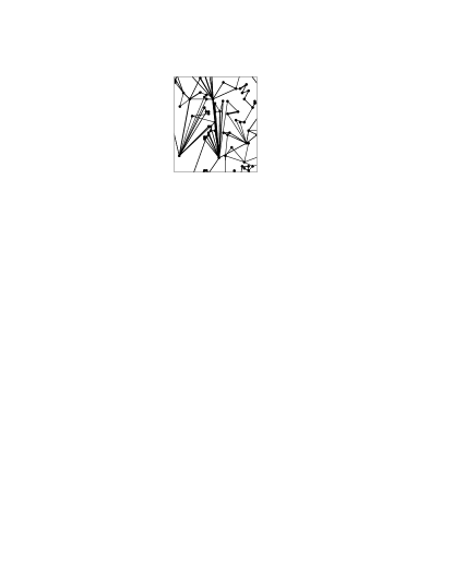
Figure 1: A fragment of a critical network ${\cal C}_{q=1.7}^{(2)}$, corresponding to a particular random conductance network with $\Delta=8.66$ on a square lattice $140\times 140$. The vertices (clusters) are shown as black circles, a thickness of a bond between two vertices $n,n^{\prime}$ is proportional to the connection number $N_{nn^{\prime}}$.

Figure 2: The probability distributions for coordination numbers $z$ and connection numbers $N$ for the same critical network, as in Fig.1.

Finally we are left with a random multiply connected network, in which every conductance is an independent random variable. The geometry of this network is highly nontrivial. Distribution functions for coordination numbers $z_{n}$, and for the “connection numbers” $N_{nn^{\prime}}$ (numbers of critical conductances, connecting vertices $n$ and $n^{\prime}$) are shown in Fig.2. It should be noted that $z_{n}$ at different vertices, as well as $N_{nn^{\prime}}$ at different links, are correlated, because vertices, corresponding to larger clusters of abridged grains, have a tendency to both larger coordination and larger connection numbers.

The statistical geometry of the critical network, no matter how complicated, is universal: it depends neither on details of the initial lattice of grains, nor on the distribution function of individual conductances. Topological properties of critical networks for all systems of a given spatial dimension $d$ are statistically equivalent. Different critical networks within the same universality class differ from each other only in the spatial scale – the correlation radius (see shklovskii ):

$$\xi^{(d)}=a[P(h_{c})]^{-\nu_{d}}\sim a\Delta^{\nu_{d}},$$ (8)

where $a$ is the typical intergrain distance, $\nu_{d}$ is the critical exponent of the correlation radius for the percolation problem in $d$ dimensions ($\nu_{2}=4/3$ and $\nu_{3}\approx 0.875$, see bunde ). The conductivity of the critical network is

$$\sigma_{q}=\frac{e^{2}}{2\pi\hbar}A^{(d)}_{q}g_{c}\left[\xi^{(d)}\right]^{2-d}\sim\frac{e^{2}a^{2-d}}{2\pi\hbar a^{d-2}}\overline{g}_{0}\Delta^{\nu_{d}(2-d)}e^{h_{c}},$$ (9)

where $A^{(d)}_{q}$ is a numerical prefactor.

Since the critical network ${\cal C}_{q}^{(d)}$ explicitly depends on the value of the parameter $q$, so does the corresponding conductivity $\sigma_{q}$. To get physically relevant $\sigma_{q\to\infty}$ one has, in principle, to extrapolate the result to $q\gg 1$. Fortunately, already for $q\gtrsim 1$ the value of $q$ affects only the numerical preexponential factor $A^{(d)}_{q}$, which rapidly converges to the true value $A^{(d)}$ as $q$ grows (the corrections are exponentially small at $q\gg 1$). The conductances with $|h_{ij}-h_{c}|\gg 1$ do not play any considerable role in the critical subnetwork, therefore for a qualitative discussion it is sufficient to choose some $q\sim 1$ and not to bother much about the effects of finite $q$. These weak and purely quantitative effects will be discussed below, when we will compare the numerical results, obtained for different values of $q$.

Temperature dependence of the critical network’s conductivity. In our problem the conductivity is also determined by the critical network, but the conductances in this network evolve with “RG time” $t$ according to the RG equations

$$\frac{d\ln g_{nn^{\prime}}^{(k)}}{dt}=-2R_{nn^{\prime}},$$ (10)

where index $k=1,\ldots,N_{nn^{\prime}}$ distinguishes different conductances, connecting the same pair $nn^{\prime}$ of vertices; $R_{nn^{\prime}}$ is the resistance of the critical network between vertices $n$ and $n^{\prime}$. It is very important, that these resistances are governed solely by the critical conductances, so that the system (10) is closed.

Let us introduce normalized variables

$$y_{nn^{\prime}}^{(k)}=h_{nn^{\prime}}^{(k)}-h_{c},\quad\tilde{t}=\frac{t}{A^{(d)}g_{c}},\quad\tilde{\sigma}=\frac{\sigma}{A^{(d)}g_{c}}\left[\xi^{(d)}\right]^{d-2}\frac{2\pi\hbar}{e^{2}},$$ (11)

then

• The critical network is reduced to a completely universal one, with the spatial scale equal to unity.

• The equations (3) take the universal form

  $$\frac{dy_{nn^{\prime}}^{(k)}}{d\tilde{t}}=-2A^{(d)}\tilde{R}_{nn^{\prime}}\left(\left\{e^{y_{ll^{\prime}}^{(p)}}\right\}\right).$$ (12)

• Initial conditions $y_{nn^{\prime}}^{(k)}(\tilde{t}=0)$ for the RG equations (12) independently take random values with a universal distribution function

  $$\tilde{P}_{q}(y)=\frac{\theta(q-|y|)}{2q}.$$ (13)

Thus we have arrived at a completely universal mathematical problem: One has to solve a set of universal equations (with universal initial conditions) for variables $y_{nn^{\prime}}^{(k)}$, defined on a random graph with universal statistical properties. As a result, the normalized conductivity $\tilde{\sigma}$ should be a universal function of the normalized time $\tilde{t}$:

$$\tilde{\sigma}_{q}=F^{(d)}_{q}(\tilde{t}),$$ (14)

the shape of this function depends only on the space dimensionality $d$ and on the parameter $q$. At $q\gtrsim 1$ the $q$ dependence is very weak and can be neglected, therefore we omit the index $q$ in what follows. Unfortunately, we were not able to find this universal function analytically, so we had to do that numerically (see below).

Coming back to the initial physical variables, we get the global conductivity of the system in the form:

$$\frac{\sigma(T)}{\sigma(T_{R})}=F^{(d)}\left[\frac{e^{2}/2\pi\hbar}{\left[\xi^{(d)}\right]^{d-2}\sigma(T_{R})}\ln\frac{T_{R}}{T}\right],$$ (15)

where $T_{R}\equiv g_{c}E_{C}$. The only nonuniversal (i.e., depending on the details of the conductances’ distribution function) ingredient in this formula is $\xi^{(d)}\sim\Delta^{\nu_{d}}$. Note also, that there is absolutely no reminiscence of the nonuniversal short-scale geometric structure of the array.

Lateral conductance of granular films. One should distinguish between thin films, whose thickness $\delta L\ll\xi^{(3)}$, and thick films with $\delta L\gg\xi^{(3)}$. The arguments of paper shkl1 (see also book shklovskii ), designed for the description of hopping conductivity in films, can be modified for our case. The true 3-dimensional behavior takes place only in thick films, where the dimensionless conductance of a square sheet of the film is $G_{\square}=\sigma^{(3)}\delta L$, and

$$\frac{G_{\square}(T)}{G_{\square}(T_{R})}=F^{(3)}\left[\left(\frac{\delta L}{\xi^{(3)}}\right)\frac{\ln(T_{R}/T)}{G_{\square}(T_{R})}\right].$$ (16)

For thin films

$$\frac{G_{\square}(T)}{G_{\square}(T_{R})}=F^{(2)}\left[\frac{\ln(T_{R}/T)}{G_{\square}(T_{R})}\right],$$ (17)

and $G_{\square}$ exponentially depends on $\delta L$:

$$G_{\square}(T_{R})=A^{(d)}\overline{g}_{0}e^{h_{c}(\delta L)},$$ (18)

where $h_{c}=h_{c}(\delta L)$ is determined as a threshold of lateral percolation in a slab of thickness $\delta L$ cut out of a three-dimensional network of all conductances with $h_{ij}<h_{c}$. The threshold condition has a form

$$\xi^{(3)}(h_{c})=c\;\delta L,$$ (19)

where the three-dimensional correlation length $\xi^{(3)}(h_{c})\sim a[(h_{c}^{(3)}-h_{c})/\Delta]^{-\nu_{3}}$, and $c\sim 1$. As a result, in the range $a\ll\delta L\ll\xi^{(3)}$ one finds

$$h_{c}^{(3)}-h_{c}(\delta L)=D\Delta(a/\delta L)^{1/\nu_{3}},$$ (20)

where $D$ is some nonuniversal numerical constant (see shklovskii ). Note, that this formula interpolates between $h_{c}^{(3)}$ in the case of a bulk, thick film, and $h_{c}^{(2)}$ in the case of a one-monolayer film.

The quasi two-dimensional critical network $\tilde{\cal C}_{q}^{(2)}$, arising in the film as a result of the $q$-procedure, centered at $h_{c}(\delta L)$, is characterized by the effective two-dimensional correlation length $\xi_{\rm eff}^{(2)}$. To estimate this length we write it in a form $\xi_{\rm eff}^{(2)}=a(\delta L/a)^{\alpha_{1}}\Delta^{\alpha_{2}}$, which follows from the scaling arguments. This expression, valid in the range $a\ll\delta L\ll\xi^{(3)}$, should match with the true two-dimensional behavior $\xi_{\rm eff}^{(2)}=\xi^{(2)}\sim\Delta^{\nu_{2}}$ at $\delta L\sim a$, and with the true three-dimensional one $\xi_{\rm eff}^{(2)}=\xi^{(3)}\sim\Delta^{\nu_{3}}$ at $\delta L\sim\xi^{(3)}$. These two matching conditions fix the exponents $\alpha_{1},\alpha_{2}$, so that we find $\alpha_{1}=1-(\nu_{2}/\nu_{3})$ and $\alpha_{2}=\nu_{2}$. As a result, $\xi_{\rm eff}^{(2)}$ can be conveniently written in a form

$$\xi_{\rm eff}^{(2)}\sim\delta L\left(\xi^{(3)}/\delta L\right)^{\nu_{2}/\nu_{3}}\gg\delta L.$$ (21)

Thus, our quasi-two-dimensional critical network is indeed effectively strictly two-dimensional, hence it belongs to the corresponding $d=2$ universality class, and the universal function is $F^{(2)}$ for all films with $\delta L\ll\xi^{(3)}$ (cf. formula (17)), not only for those, consisting of just one monolayer of grains.

Numerical results. In this Letter we present the numerical results only for the two-dimensional case. For determination of the function $F^{(2)}_{q}(\tilde{t})$ we have generated random $L\times L$ square arrays of conductances with distribution $P(h)=\theta(\sqrt{3}\Delta-|h|)/2\sqrt{3}\Delta$ for different $20<L<140$ and $0<\Delta<8.66$. For the samples with large $\Delta$ we constructed critical networks ${\cal C}_{q}^{(2)}$ with $0.5<q<2$, and numerically solved the system of equations (12) and (4) on these networks, which are very much smaller arrays, than the initial ones. Note, that only due to this truncation of the array, as well as to the fact, that the conductances of the critical network are all of the same order of magnitude, the problem becomes feasible. The numerical solution of the full set of Kirchhof equations for a reasonably large array of strongly different conductances would be practically impossible. Thus, the concept of the critical network turns out to be crucially helpful not only for understanding of basic physics, but also for the numerics.

The main result – the dependence of the conductivity on $\ln(T_{R}/T)$ for different values of $\Delta$ is shown in Fig.3. One can see that this dependence becomes universal already at $\Delta\sim 3-4$: the difference between curves with $\Delta=3.47$ and $\Delta=8.66$ is negligible, so we can with reasonably high accuracy identify the last one with the universal function $F^{(2)}(\tilde{t})$. In the range $0<\tilde{t}<0.5$ it is approximately linear with a slope, corresponding to an effective coordination number $z_{\rm eff}\approx 3.2$, which is consistent with the statistics of coordination, shown in Fig.2. Note, that $z_{\rm eff}$ is universal and does not depend on the coordination number $z$ of the initial lattice. At $\tilde{t}>0.5$ the slope starts to decrease rapidly, and $F^{(2)}(\tilde{t})$ goes to zero at $\tilde{t}_{c}\approx 1.2$. Unfortunately, the problem of finding the critical exponent, which characterizes the behavior of $F^{(2)}(\tilde{t})$ at $\tilde{t}\to\tilde{t}_{c}$, seems to be numerically not feasible.

Figure 3: Dependence of the normalized conductance per square for a thin film on the parameter $t=\ln(T_{R}/T)$ for different standard deviations $\Delta$ of the logarithms of intergrain conductances. $M$ is the number of samples in the averaging ensemble. In all cases $q=1.7$ and $L\gg\xi^{(2)}(\Delta)$. (a) – $\Delta=0.14$, $L=50$, $M=150$; (b) – $\Delta=0.58$, $L=50$, $M=150$; (c) – $\Delta=1.16$, $L=50$, $M=300$; (d) – $\Delta=2.31$, $L=80$, $M=300$; (e) – $\Delta=3.47$, $L=100$, $M=400$; (f) – $\Delta=8.66$, $L=140$, $M=400$. in all cases $q=1.7$ and $L\gg\xi^{(2)}(\Delta)$. The thick line – universal function $F^{(2)}(\tilde{t})$.

We also have checked the accuracy of the method from the point of view of finite size and finite $q$ corrections. For an array $40\times 40$ with $\Delta=1.734$ we were able to perform the straightforward calculations (involving the entire array) and compare their results to those, obtained on truncated ${\cal C}_{q}$-networks. The results of this comparison, shown in Fig.4, demonstrate a very good accuracy already at moderate values of $q=1.7$. This accuracy is reached at the network, which includes only about a half of all conductances of the array. Note, that although the condition $q\ll\Delta$, required for general distributions $P(h)$, is obviously not satisfied in this particular simulation, for the rectangular shape of $P(h)$, used here, the strong inequality can be substituted by a milder condition $q<\sqrt{3}\Delta$.

For a sample $140\times 140$ with $\Delta=8.66$ (the same realization, as used in Figs.1,2) we performed the calculations with different values of $q$. The results, shown in Fig.5 demonstrate fast convergence of the procedure: the difference between $F_{q}^{(2)}$ for $q=1.7$ and $q=1.9$ is already very small, so that using $q=1.7$ procedure for evaluating the universal function $F^{(2)}$ is a very good approximation.

From general arguments it is clear that to get self-averaging results, one should use arrays with size $L>\xi^{(2)}$. In Fig.6 we have plotted functions $F^{(2)}(\tilde{t})$, found for arrays with the same $\Delta=8.66$, but with different sizes $L$. For these arrays one expects $\xi^{(2)}\sim C[P(h_{c})]^{-\nu_{2}}=C\cdot 30^{4/3}=93C$ (with unknown numerical coefficient $C$). We see that for $L>100$ the curves become almost identical, so we conclude that $C\sim 0.5-1$ and square arrays with $L>[P(h_{c})]^{-\nu_{2}}$ can empirically be considered as large enough.

Figure 4: Comparison of the solutions of the full set of equation for the $40\times 40$ sample with $\Delta=1.734$ (solid line) and the set, truncated according to the $q$-procedure with $q=1.7$ (broken line).

Figure 5: Comparison of the solutions, using $q$-procedure with different $q$. One can see that the difference between $q=1.7$ and $q=1.9$ results is already negligible.

Figure 6: Comparison of solutions for different lattice sizes $L$. All curves are obtained for largest standard deviation $\Delta=8.66$ by the $q$-procedure with $q=1.7$, and averaged over $M=400$ realizations.

In principle, the proper thing to do would be an accurate extrapolation of finite-$q$ and finite-$L$ results to $q=\infty$ and $L=\infty$. Unfortunately, the complexity of the numerical solution at large $\Delta$, $q$, and $L$ did not allow us to reach the accuracy, necessary to such an extrapolation. The larger $q$ is chosen for $q$-procedure, the less stable and precise the calculation of $R_{ij}$ becomes. This instability limits $q$ by about $q=2$. Another precision limitation is rapid increase of computational complexity with increase of $L/\xi^{(2)}$. The mentioned difficulties limit the accuracy of each curve by about 5%, which is comparable with the separation of neighboring curves on our plots, making the extrapolation procedure senseless. However, since a rapid convergence of the results is observed, we believe that the universal curve $F^{(2)}(\tilde{t})$ lies within the same 5% error interval near the curve with $\Delta=8.66$, $L=140$.

Conclusions. Thus, the dependence of conductivity $\sigma$ on $\ln T$ for strongly disordered arrays of grains is nonlinear and universal, contrary to the case of a regular array, for which this dependence is linear, with a nonuniversal slope. The sign of the curvature of this nonlinear function is such, that the effects of strong disorder seem to improve the agreement between the theory and the experimental law (1). Unfortunately, the available experimental data is still not sufficient for a direct quantitative comparison of theory and experiment. In particular, it is hard to make reliable estimates for $T_{R}$ and $G_{\square}(T_{R})$. It is also worth reminding that the one-loop RG, which is the basis of the present theory, is valid at temperatures well above the metal-insulator transition.

The universality of the temperature dependence of the conductivity is the direct consequence of the universality of the critical network, which carries the current in a highly inhomogeneous system. This critical network in a granular film appears to be effectively two-dimensional, if the film’s thickness $\delta L$ is less than the three-dimensional correlation length $\xi^{(3)}\sim a\Delta^{\nu_{3}}$, the latter being large at high level of disorder.

We are grateful to M.V.Feigelman, D.S.Lyubshin and M.A.Skvortsov for useful discussions. Special thanks are due to D.S.Lyubshin for his invaluable advises, concerning the numerical aspect of this work. The project was supported by the Program “Quantum Macrophysics” of RAS and by RFBR grant 06-02-16533.

References

- (1) T.Chui et al, Phys. Rev. B 23, 6172 (1981).
- (2) R.W.Simon et al, Phys. Rev. B 36, 1962 (1987).
- (3) A.Gerber et al, Phys. Rev. Lett., 78, 4277 (1997).
- (4) K. B. Efetov and A. Tschersich, Europhys. Lett. B 59, 114 (2002); Phys. Rev. B 67, 174205 (2003).
- (5) I. S. Beloborodov, et al, Phys. Rev. Lett. 91, 246801 (2003).
- (6) A.Altland, L. I. Glazman, and A. Kamenev, Phys. Rev. Lett. 92, 026801 (2004).
- (7) J. S. Meyer, A. Kamenev and L. I. Glazman, Phys. Rev. B 70, 045310 (2004).
- (8) M.V.Feigelman, A.S.Ioselevich and M.A.Skvortsov, Phys. Rev. Lett. 93, 136403 (2004).
- (9) J.Zhang and B.I.Shklovskii, Phys.Rev. B 70, 115317 (2004)
- (10) M.V.Feigelman, A.S.Ioselevich, JETP Letters 81, 341 (2005).
- (11) V.I.Kozub et al, JETP Letters 81, 287 (2005)
- (12) I.S.Beloborodov, A.V.Lopatin, V.M.Vinokur, Phys.Rev. B 72, 125121 (2005).
- (13) T.B.Tran et al, Phys.Rev.Lett., 95, 076806 (2005).
- (14) V. A. Ambegaokar, U. Eckern and G. Schön, Phys. Rev. Lett. 48, 1745 (1982)
- (15) S.Kirkpatrick, Rev. Mod. Phys. 45, 574 (1973).
- (16) B.I.Shklovskii and A.L.Efros Electronic Properties of Doped Semiconductors, Springer, Berlin, (1984)
- (17) A.Bunde and S.Havlin, Percolation I, in Fractals and Disordered Systems, eds. A.Bunde and S.Havlin, Springer, Berlin (1996)
- (18) B.I.Shklovskii, Phys. Lett. 51 A, 289 (1975)