Energy Transport in Weakly Anharmonic Chains
Kenichiro Aoki∗, Jani Lukkarinen⋆,
Herbert Spohn†
∗Department of Physics, Keio University,
4–1–1 Hiyoshi, Kouhoku–ku, Yokohama 223–8521, Japan,
e-mail: ken@phys-h.keio.ac.jp
⋆Zentrum Mathematik, TU München,
D-85747 Garching, Germany,
e-mail: jlukkari@ma.tum.de
†Zentrum Mathematik, TU München,
D-85747 Garching, Germany,
e-mail: spohn@ma.tum.de
Abstract.
We investigate the energy transport in a one-dimensional lattice
of oscillators with a harmonic nearest neighbor coupling and a
harmonic plus quartic on-site potential. As numerically observed
for particular coupling parameters
before, and confirmed by our study, such chains satisfy Fourier’s
law: a chain of length coupled to thermal reservoirs at both
ends has an average steady state energy current proportional to
. On the theoretical level we employ the Peierls transport
equation for phonons and note that beyond a mere exchange of labels
it admits nondegenerate phonon collisions. These
collisions are responsible for a finite heat conductivity. The
predictions of kinetic theory are compared with molecular dynamics
simulations. In the range of weak anharmonicity, respectively
low temperatures, reasonable agreement is observed.
1 Introduction
In their seminal work of 1955, Fermi, Pasta, and Ulam [1]
investigate the relaxation to
equilibrium for a chain of coupled anharmonic oscillators,
by exploiting the then newly available
electronic computational devices. We refer to the informative
memorial volume [2]. Related to their study
is the issue of energy transport along the chain, which
is modelled by coupling a chain of length to thermal reservoirs
at both ends. With increased computational power at hand such
studies have been revived and carried through in considerable
detail. Excellent reviews are in print [3, 4] and here we
only highlight, somewhat crudely, the
main findings:
(i) There are chains for which Fourier’s law holds, in the sense
that the steady state energy flux .
ii) There are chains with anomalous heat conduction, for which the
energy flux exhibits a power law dependence on which differs
from .
iii) If the interaction depends only on the relative
displacements, anomalous heat conduction seems to be the
rule.
iv) In some models the conductivity depends on the details of the
coupling to the thermal reservoirs.
While the amount of data available is impressive, it is generally agreed that there is very little theory which would serve as a guideline. The harmonic chain can be solved exactly with the result that is independent of [5]. For the harmonic chain with random masses the transport for a given wave number is proportional to , , with as . Thus the average energy current depends on the precise spectral statistics of the thermal reservoir [6, 7]. For anharmonic chains there are attempts to predict the exponent for the anomalous heat conduction through mode-coupling theory [8, 9].
In our note we follow the strategy of Peierls, who argues that in case of weak nonlinearity one can use a Boltzmann type transport equation for the computation of the thermal conductivity. For anharmonic crystals in three dimensions phonon kinetic theory is well supported through theory [10, 11, 12] and also experimentally [10, 13]. Whether kinetic theory is applicable to a weakly anharmonic chain is somewhat tentative. There is no difficulty in writing down the appropriate transport equation. Its collision term ensures energy and momentum conservation in a phonon collision. To progress further an analysis of the solution manifold to both conservation laws becomes necessary. Firstly one has the trivial solutions in which the two colliding phonons merely exchange their label. For the label exchanging solutions the collision operator vanishes. However, as we first learned from Lefevere and Schenkel [14], there is in addition a non-perturbative solution, which leads to nondegenerate collisions. As will be explained in more detail, with this input kinetic theory predicts a finite, non-zero, thermal conductivity even for a chain.
As we learned later on, Pereverzev [15] has already applied kinetic theory to the FPU -lattice, for which the potential energy depends only on the relative displacements. For this model he obtains the non-perturbative solution and argues, based on the linearized transport equation, that the energy current correlation has a power law decay as . Thus the heat transport is anomalous with . In our contribution we will be concerned with regular transport only.
To keep the model as simple as possible we will study the harmonic chain with a small quartic on-site potential. Equivalently, one may consider a fixed anharmonicity but “low” temperatures. We regard the thermal conductivity to be defined through the Green-Kubo formula and work out the predictions of kinetic theory in fair detail. To explicitly compute the conductivity one has to invert the linearized collision operator. This is not completely straightforward and we have to be satisfied with some estimates, which however turn out to be sufficient for our purposes. The predictions of kinetic theory will be compared with molecular dynamics simulations. In fact, kinetic theory does rather well, with a range of validity larger than expected on the basis of purely theoretical arguments.
2 The Green-Kubo formula, scaling properties
The anharmonic chain is governed by the Hamiltonian
| (2.1) |
Here is the deviation from the rest position and the momentum of the -th particle. We choose units such that the mass of a particle equals 1. and characterize the harmonic on-site and nearest neighbor interaction, respectively. and it has the dimensions of a frequency. To have a stable harmonic part of we require
| (2.2) |
In the border case , the harmonic part can be written as and thus depends only on the relative displacement. is the strength of the quartic on-site potential.
The particular case , is studied in great detail in [16], in which case kinetic theory is applicable at low temperatures. For our purposes it is of importance to add the extra parameter , since it is retained in the kinetic limit. Thereby one can compare the theoretical predictions with molecular dynamics simulations in their -dependence.
To (2.1) we associate the local energy
| (2.3) |
Then
| (2.4) |
with the energy current across the bond to given by
| (2.5) |
The equilibrium state for (2.1) is with denoting temperature. Equilibrium expectations are denoted by . We define the total energy current correlation through
| (2.6) |
By stationarity of , . According to Green-Kubo the thermal conductivity at temperature is defined by
| (2.7) |
Regular transport in the sense of Fourier’s law requires that .
does not depend on all of its parameters separately. To find the dependence out we transform to new variables as
| (2.8) |
Then , are solutions to Hamilton’s equations of motion for the Hamiltonian
| (2.9) |
In addition,
| (2.10) |
Therefore,
| (2.11) |
which by (2.7) implies for the conductivity
| (2.12) |
Setting , yields the scaling form
| (2.13) |
In our molecular dynamics simulations, see Sect. 5, we set and . On the other hand, for the kinetic limit the natural choice is and fixed inverse temperature . Inserting , in (2.12) one arrives at
| (2.14) |
Thus the limit on the left corresponds to the limit of on the right hand side, which will be studied in the following section.
3 Energy current-current correlation in the kinetic limit
In this section we set . To study the kinetic limit it is convenient to switch to Fourier space. Let be the first Brillouin zone of the lattice dual to . For we set
| (3.1) |
with the inverse
| (3.2) |
We decompose
| (3.3) |
The harmonic part has the dispersion relation
| (3.4) |
, , are concatenated into a single complex-valued field through
| (3.5) |
Notationally it will be convenient to also define
| (3.6) |
Then the equations of motion read
| (3.7) |
In these new variables the harmonic part of the energy becomes
| (3.8) |
and the total current, , becomes
| (3.9) |
We plan to study the energy current correlation (2.6) in the limit of small . Since in equilibrium , it holds
| (3.10) |
where refers to expectation with respect to the perturbed equilibrium measure , the total current, in the infinite volume limit. For small we can ignore the quartic on-site potential in the average . Thus is replaced by the Gaussian measure , which is uniquely characterized through its covariance
| (3.11) |
The state is not invariant under the mechanical time evolution and we have to understand how for small such a non equilibrium measure evolves in time. Instead of let us consider as initial state an arbitrary translation invariant Gaussian measure with covariance
| (3.12) |
compare with (3). Its two-point function at time is given by
| (3.13) |
which defines . In particular, by (3.9),
| (3.14) |
For , one has . For small the time variation of is on the time-scale . Thus one expects that the following limit exists,
| (3.15) |
and that the limit Wigner function evolves according to the spatially homogeneous Boltzmann equation
| (3.16) |
with initial conditions . Here, and later on, we use the shorthand , , , , . In Appendix A we explain the second order diagrammatic expansion in , mostly to make sure that the collision strength is correct.
By the argument in Appendix 18.1 of [12], energy and momentum conservation in (3) can be satisfied only if
| (3.17) |
i.e., only for phonon number conserving collisions. Hence (3) simplifies to
| (3.18) |
Clearly, the equilibrium Wigner function
| (3.19) |
is a stationary solution for (3). Since according to (3.10) and (3) only small deviations from equilibrium are needed, we linearize the collision operator as
| (3.20) |
Then
| (3.21) |
For this particular choice of linearization in .
Let . Then
| (3.22) |
Let and let be the scalar product in . Then, with denoting the solution to (3) for the initial condition , one has
| (3.23) |
Integrating over time one concludes that
| (3.24) |
Combining with (2.14) yields as the final result
| (3.25) |
The inner product on the right depends only on . The prefactor is slightly misleading, since is proportional to . Hence
| (3.26) |
with .
(3) can rephrased as the asymptotics of the scaling function from (2.13),
| (3.27) |
In other words
| (3.28) |
for small . Our argument provides no indication over which range (3.28) is a valid approximation. In fact, even the claim (3.25), (3.26) is tentative. The diagrammatic expansion from Appendix A relies on the separation into leading and subleading diagrams. For a three-dimensional lattice such a separation is convincing and can be checked for special diagrams. The oscillatory time integrals for the chain have a slower decay and the rough estimates used so far are not sufficient to justify the separation into leading and subleading diagrams, which we have assumed here. On the other hand, there could very well be cancellations which are difficult to access through the expansion in Feynman diagrams. Also we need the validity of the kinetic equation only close to thermal equilibrium. In view of this situation a molecular dynamics simulation is in demand.
4 Thermal conductivity from the one-dimensional Boltzmann equation
The linearized collision operator of (3) corresponds to the quadratic form
| (4.1) |
We use momentum conservation to integrate over . For energy conservation we thus need the solutions to
| (4.2) |
The obvious solutions are
| (4.3) |
Expanding (4.2) to first order in , as noticed in [14], there is yet a further, non-perturbative solution given by
| (4.4) |
This suggests to write, in general,
| (4.5) |
Indeed, for every there exists a unique function , which is continuous, one-to-one, and satisfies
| (4.6) |
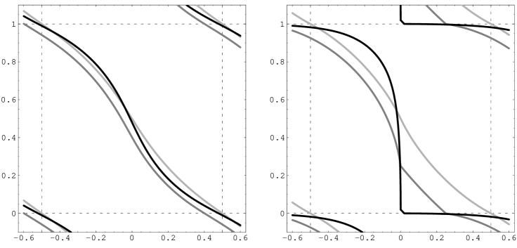
is called the non-perturbative solution. In Fig. 1 we display a few non-perturbative solutions at and for three values of . For small one finds
| (4.7) |
which reasonably well approximates the left hand of Fig. 1.
Inserting the solutions (4.3) and (4.5) to energy conservation into (4) splits the linearized collision operator as the sum
| (4.8) |
By symmetry, for the label exchanging solution for all . Hence and energy conservation in (4) will be evaluated always at .
In phonon kinetic theory it is customary to distinguish between normal and umklapp processes. We choose the convention that , . Then a process is called normal if , while it is umklapp if . By this definition, the curves in Fig. 1 are divided into a normal piece and an umklapp piece. For example, at , one has and . If the two terms have opposite sign, the collision process is normal and otherwise it is umklapp. In our context such a division looks artificial. In fact we will find that both, normal and umklapp, processes contribute to the thermal conductivity.
We turn to the zero subspace of , i.e., to solutions of in . By (4), clearly they must be collisional invariants in the sense that
| (4.9) |
for all . The obvious solutions are
| (4.10) |
We expect that there are no further solutions, but no proof is available, at present. This is an important issue, since speaking in general, the number of collisional invariants is the crucial information on the long-time behavior of a kinetic equation. At , does not depend on and as a consequence the zero subspace of becomes infinite-dimensional consisting of all ’s satisfying .
We integrate in (4) over and . For the volume element with respect to we need
| (4.11) | |||
Hence
| (4.12) |
and carries an explicit prefactor , as claimed in (3.26).
To obtain the thermal conductivity (in the kinetic regime) one has to invert , which can be achieved only numerically and which is not completely straightforward because of the constraint due to energy conservation. However for small , say up to , more modest means already suffice. By Jensen’s inequality one has
| (4.13) |
with . For one obtains
| (4.14) |
and
| (4.15) |
Combing (3.25) and (4.13), (4.14), (4) yields
| (4.16) |
for small .
For numerical inversion of at we expand in a basis of the form , , and, instead of , obtain the prefactor in (3.26) as with a stable value over the range . As can be seen from Fig. 1, even at the approximate solution (4.7) is rather accurate. Therefore is expected to depend only weakly on . Our claim is supported by the lower bound
| (4.17) |
. For this particular choice of the variational function the singular denominator in (4) is cancelled exactly and the numerical integration, using the true non-perturbative solution, becomes routine. The lower bound to drops from at to at . More details on the linearized collision operator can be found in [17].
5 Thermal conductivity from molecular dynamics

Kinetic theory is expected to be valid for small dimensionless coupling and large system size. How small a coupling and how large a system size can be explored only through molecular dynamics simulations. To this end, we compute thermal conductivities for various parameters of the anharmonic chain (2.1). We set , . Then the infinite volume conductivity depends only on and kinetic theory becomes valid in the limit , compare with Sects. 2 and 3. In particular,
| (5.1) |
for small with and slowly dropping to smaller values as is increased.
To numerically determine the thermal conductivity we take a chain of finite length, , and attach thermostats at both ends. We use free boundary conditions, which means at the boundaries, but the physical results are insensitive to this particular choice of boundary conditions. We adopt deterministic thermostats which generalize those of Nosé–Hoover [18, 19], and follow the methods used for the chain when [16, 20]. The non–equilibrium steady state is achieved by integrating the equations of motion and physical observables are measured by averaging over time after waiting for a sufficiently long equilibration time span. The integration is performed numerically using standard algorithms, such as Runge–Kutta, with time steps of . samples are taken to obtain the average values of physical observables. The results do not depend on the time step size. A non–equilibrium steady state has as its parameters the boundary temperatures, , and . The local temperature is defined through the relation .
In principle, a single non–equilibrium state suffices to obtain . To determine with enough accuracy we employ a more elaborate procedure. We choose boundary conditions with varying temperature gradients, , but with the same temperature close to the midpoint. We can then check that the average current is linear in and obtain for given , and , as illustrated in Fig. 2. The temperature gradient needs to be computed away from the boundaries because of jumps in the temperature at both ends, see Sect. 6 for a discussion. Since local energy is conserved and there are no internal heat sinks or sources, the average current is constant throughout the system. We increase and examine if the bulk limit is reached to finally extract for given . Bulk behavior had already been observed when [20, 21], and we do so also in the present study.


Naively, it would seem that weak coupling physics should be easy to simulate. The computational difficulties arise because the mean free path inevitably becomes large and the relaxation towards the steady state becomes slow, which demands to carry out the simulation for large system sizes and sufficiently long times. These factors limit the range of accessible parameters values. To elucidate these points and also to understand the kinetic theory aspects of this system better, we analyze the statistical properties of the system in more detail. To judge the required system size we have to estimate the mean free path . It is not a sharply defined quantity. Following Ziman [10] we set
| (5.2) |
where is the specific heat and the average speed of phonons. In the harmonic approximation one obtains . Kinetically the equilibrium phonon number density equals , which suggests to set
| (5.3) |
with the following expansion for small ,
| (5.4) |

The speed of phonon propagation can also be measured directly from the time and space dependences of the autocorrelation function in thermal equilibrium [9, 16]. The velocity of the peaks in the correlation function is equated with the average phonon velocity relevant for thermal transport. An example is shown in Fig. 3. The measured velocities can be compared to the kinetic result in (5.4), which is done in Fig. 4. Perfect agreement is not expected for a number of reasons. First, there is no unique definition of the average speed of phonons so that there is no guarantee that the average (5.3) is precisely what we measure in the molecular dynamics simulations as in Fig. 3. Furthermore, the kinetic approximation for does not include the effects of anharmonicities and should strictly hold only in the limit . Given these constraints, the agreement between the simple formula (5.3) for and the simulation results in Fig. 4 is fairly satisfactory.
From the above discussion and using (5.1) we obtain
| (5.5) |
for small , . From the measured values of (see Figs. 4 and 5), can be determined according to (5.2). ranges then from at , to at , . In the simulations the system size is varied up to a few thousand depending on the parameters. Therefore, in our simulations, we have been able to achieve in the parameter range probed here. When and are of the same order, it is not clear a priori if the bulk limit has been reached. In the subsequent section, we provide an argument that we might still be able to estimate the conductivity in such cases, even when .

One distinctive qualitative feature of kinetic theory is the leading dependence of , see (5.1). To compare the molecular dynamics simulation results with kinetic theory, we need to keep in mind that the agreement should hold only when is small and the power law becomes exact when . In Fig. 5 the comparison is made and we note a surprisingly good agreement, which improves as the temperature is lowered, as to be expected.
6 Steady state temperature profile
A second quantity of physical interest is the average temperature profile. If difference in the boundary temperatures, , is small, then the profile is approximately linear. For larger the temperature dependence of will be seen. As is further increased, local equilibrium will break down eventually [22]. We begin with working out the temperature profile as predicted by the transport equation.
The space-time dependent version of the Boltzmann equation (3) reads
| (6.1) |
, where the collision operator is local in , i.e., it acts only on the wave number . Under (6.1) the phonon number density
| (6.2) |
and the energy density
| (6.3) |
are locally conserved. The former one we regard as spurious, since it has no analogue on the microscopic level.
Following the standard hydrodynamic scheme, since there are no convective terms, the long time behavior of (6.1) is thus dictated by the solution of the coupled nonlinear diffusion equations
| (6.4) |
Here , are “chemical potentials” labelling the stationary solutions, , of (6.1) as
| (6.5) |
for , where for and for . Then with
| (6.6) |
In (6.4) we insert the inverse function as defined on , which is uniquely specified because of convexity. Secondly, is the matrix of Onsager coefficients as given through a Green-Kubo formula analogous to (3). Following in spirit the arguments from [12] one obtains
| (6.7) |
with the linearized collision operator
| (6.8) |

At , is independent of , which results in an important simplification. Let us consider the steady state problem for (6.4) in the slab with boundary conditions , , , . Then the solution is given by
| (6.9) |
In particular the steady state energy flux is
| (6.10) |
For a small temperature difference, , , one has in approximation
| (6.11) |
where in agreement with (3.25).
In molecular dynamics simulations the two ends of the chain, and , are coupled to thermal reservoirs with of order or less. The local value of is extracted from the simulation. A simple test is provided by the momentum covariance. If locally the Wigner function has the form , then
| (6.12) |
which reduces to for . Expanding (6.12) in results in . Numerically, the steady state momentum correlation is indeed strongly peaked at and decays rapidly. The simulations therefore indicate that is small compared to and hence one can safely set . An example for off-diagonal correlations obtained from molecular dynamics simulations is shown in Fig. 6 and, in this case, . This quantity is close to but not quite zero. This may be due to being small, but not quite zero, or due to finite size corrections to local equilibrium.

In Fig. 7 we display a numerically generated steady state profile. One notes that the profile lies slightly below the linear interpolation. Indeed, (6.9) claims that is linear. The dashed line is the corresponding fit. The excellent agreement is a further confirmation for being small.
A generic temperature profile consists of three pieces: there are two boundary jumps of equal size and concentrated over a few lattice spacings and there is an, in essence, linear bulk piece. Only if the effective temperature difference is large, one observes deviations from linearity, as for example in Fig. 7. According to [5], and as easily extended to the case under study, in the harmonic limit boundary jumps would be exponentially localized and the bulk piece would be flat. The observed temperature profile deviates significantly from this harmonic limit for all data points from Fig. 5 in always having a nonzero slope.
The equal size boundary jumps are easily understood in the context of Langevin reservoirs. The leftmost particle, , is then governed by the Langevin equation
| (6.13) |
where is the friction coefficient and white noise such that . A corresponding equation holds for the rightmost particle, , with replaced by . In the steady state , which implies
| (6.14) |
where is the steady state current for chain length . Similarly
| (6.15) |
In particular, the boundary jumps are equal.
To understand the full structure of the steady state one may resort to (6.1) restricted to the slab . Then the steady state Wigner function, , satisfies with the following boundary conditions at the two ends, ,
| (6.16) |
where we assumed thermal sources together with complete absorption. To obtain the steady state profile on this basis would need considerable numerical effort. Therefore we turn to a very much simplified model, which however retains the gross features of the steady state.
Energy is transported to the right with velocity and to the left with velocity . Locally the velocity may switch its orientation randomly with rate . Then the mean free path is and, as we will see, Fourier’s law holds with conductivity . In the steady state the average energy density satisfies
| (6.17) |
The local energy is , which we identify with the local temperature. The energy current is then . Energy is injected at and absorbed at , i.e.
| (6.18) |
where partial absorption could readily be included. Comparing to the case and , one concludes that the imposed right boundary temperature is and correspondingly the imposed left boundary temperature . The solution to (6), (6.18) reads
| (6.19) |
which yields the temperature profile
| (6.20) |
and the steady state current for slab length as
| (6.21) |
Thus at both ends the boundary jump equals and the effective temperature difference is . Hence
| (6.22) |
Thus, even if , the correct bulk current is extracted through (6.22). Of course, as for fixed the mean free path increases, so does the relaxation time and longer simulation times would be needed.
To come back to the molecular dynamics computation, the simulation time is sufficiently long so that the steady state is reached. For most of the data presented, we obtain the conductivity from lattices with and are confident that they should be reliable. At data with small are computed for lattices with . Given the reasoning within the simplified model and the tendency of the data for larger , we believe that a reasonable estimate for the conductivities has been obtained even for these cases.
7 Conclusions
The Boltzmann-Peierls equation retains the exact dispersion relation and the type of nonlinearity of the Hamiltonian model. For example, had we considered a cubic nonlinearity, then Eq. (3) would be quadratic in . For a nonlinearity which depends on the nearest neighbor relative displacements there would appear the additional factor in the collision rate. It is remarkable that with this input the qualitative features of the “low” temperature thermal conductivity are so well recovered.
It seems to us that the Boltzmann-Peierls equation has never been tested in comparable precision before. The peak time for the experimental investigation of phonon thermal conductivity was in the late 50’ies and early 60’ies. A quantitative comparison with the theory was hampered from two sides: (1) The dispersion relation and the anharmonicities of a given dielectric crystal are not so readily available. (2) One needs considerable numerical effort to reliably obtain the thermal conductivity from the transport equation. Thus mostly one had to be satisfied with qualitative predictions, as for example the -dependence of the thermal conductivity in the presence of only three-phonon collisions [10]. More recently, molecular dynamics simulations have become available, for example see [23] and references therein. Compared to these more material science oriented studies, we achieve a much larger system size, due to one instead of three spatial dimensions, and we test the simulation data directly against the transport equation without further approximations.
Acknowledgments. KA was supported in part by Grant–in–Aid for Scientific Research from the Ministry of Education, Culture, Sports, Science and Technology of Japan. JL and HS thank Jean Bricmont, Antti Kupiainen, Raphael Lefevere, and Alain Schenkel for most instructive discussions, which merged into the present study.
Appendix A Appendix
We follow Sect. 11 of [12]. The initial measure is translation invariant and uniquely characterized by the covariance of (3). We want to establish that
| (A.1) |
for small .
By (3) the vertex weight is given by
| (A.2) |
We use the expansion through Feynman diagrams as obtained from the iteration of (11.7) in [12]. Since the Hamiltonian has a quartic nonlinearity, each interaction leads to a branching into 3 lines, compare with Fig. 5 of [12].
To order we simply have . The order
term is purely imaginary, thus vanishes, because to
every diagram there is its complex conjugate, denoted by
c.c.. Thus we are left with the order . It has
8 ways of branching. For a given branching there are 15 Gaussian
pairings and 8 possible orientations of the internal lines, which
in total amounts to 960 diagrams. They will be divided into
subleading and
leading.
(i) There are 144 diagrams of the type
We set . Their sum is then
| (A.3) |
(ii) There are 144 diagrams of the type
Their sum is
| (A.4) |
(iii) There are 288 diagrams of the type
Their sum is
| (A.5) |
In (i) and (ii) the terms independent of cancel each other.
The remaining terms are proportional to and
thus of order after time-integration. We are left with
384 leading diagrams.
(iv) The gain term results from 96 diagrams of the type
Their sum is
| (A.6) |
(v) The loss term results from 288 diagrams of the type
Their sum is
| (A.7) |
In (iv) and (v) we use that
| (A.8) |
when integrated against a smooth, rapidly decreasing test function. By adding (iv) and (v) one obtains the collision operator from Eq. (3) with the prefactor .
References
- [1] E. Fermi, J. Pasta, and S. Ulam, Studies in nonlinear problems, I, in Nonlinear Wave Motion, A.C. Newell, ed. (American Mathematical Society, Providence, RI, 1974), pp. 143. Originally published as Los Alamos Report LA-1940 in 1955.
- [2] Focus Issue: The “Fermi-Pasta-Ulam” problem – the first 50 years, Chaos 15 (1), (2005)
- [3] F. Bonetto, J.L. Lebowitz, and L. Rey-Bellet, Fourier’s law: A challenge to theorists, in Mathematical Physics 2000, A. Fokas, A. Grigoryan, T. Kibble, and B. Zegarlinski, eds., p. 12, Imperial College Press, London, 2000.
- [4] S. Lepri, R. Livi, and A. Politi, Thermal conductivity in classical low-dimensional lattices, Phys. Rep. 377, 1 (2003)
- [5] Z. Rieder, J.L. Lebowitz, and E. Lieb, Properties of a harmonic crystal in a stationary nonequilibrium state, J. Math. Phys. 8, 1073 (1967)
- [6] A. Casher and J.L. Lebowitz, Heat flow in regular and disordered harmonic chains, J. Math. Phys. 12, 1701 (1971)
- [7] J.B. Keller, G.C. Papanicolaou, and J. Weilenmann, Heat conduction in a one-dimensional random medium, Comm. Pure Appl. Math. 32, 583 (1978)
- [8] O. Narayan and S. Ramaswamy, Anomalous heat conduction in one-dimensional momentum-conserving systems, Phys. Rev. Lett. 89, 200601 (2002)
- [9] S. Lepri, R. Livi, and A. Politi, On the anomalous thermal conductivity of one-dimensional lattices, Europhys. Lett. 43, 271 (1998)
- [10] J. M. Ziman, Electrons and Phonons, Clarendon Press, Oxford, 1960.
- [11] V.L. Gurevich, Transport in Phonon Systems, North-Holland 1986.
- [12] H. Spohn, The phonon Boltzmann equation, properties and link to weakly anharmonic lattice dynamics, J. Stat. Phys., to appear, arXiv:math-phys/0505025
- [13] T. M. Tritt, Thermal Conductivity, Theory, Properties, Applications. Physics of Solids and Liquids, Springer, Berlin, 2005.
- [14] R. Lefevere and A. Schenkel, Normal heat conductivity in a strongly pinned chain of anharmonic oscillators, J. Stat. Mech. (2006) L02001
- [15] A. Pereverzev, Femi-Pasta-Ulam lattice: Peierls equation and anomalous heat conductivity, Phys. Rev. E 68, 056124 (2003)
- [16] K. Aoki, D. Kusnezov, Non-equilibrium statistical mechanics of classical lattice field theory, Ann. Phys. 295, 50 (2002)
- [17] J. Lukkarinen and H. Spohn, in preparation.
- [18] S. Nosé, A unified formulation of the constant temperature molecular dynamics methods, J. Chem. Phys. 81, 511 (1984)
- [19] W. G. Hoover, Canonical dynamics: equilibrium phase-space distributions, Phys. Rev. A 31, 1695 (1985)
- [20] K. Aoki, D. Kusnezov, Bulk properties of anharmonic chains in strong thermal gradients: non-equilibrium theory, Phys. Lett. A 265, 250 (2000)
- [21] B. Hu, B. Li, H. Zhao, Phys. Rev. E 61 3828 (2000)
- [22] K. Aoki, D. Kusnezov, Violations of local equilibrium and linear response in classical lattice systems, Phys. Lett. A309 377 (2003)
- [23] A. J. H. McGaughey and M. Kaviany, Thermal conductivity decomposition and analysis using molecular dynamics simulations. Part I. Lennard-Jones argon, Int. J. Heat and Mass Transfer 47, 1783 (2004)