Squeezing in the weakly interacting Bose condensate

Abstract

We investigate the presence of squeezing in the weakly repulsive uniform Bose gas, in both the condensate mode and in the nonzero opposite-momenta mode pairs, using two different variational formulations. We explore the $U(1)$ symmetry breaking and Goldstone’s theorem in the context of a squeezed coherent variational wavefunction, and present the associated Ward identity. We show that squeezing of the condensate mode is absent at the mean field Hartree-Fock-Bogoliubov level and emerges as a result of fluctuations about mean field as a finite volume effect, which vanishes in the thermodynamic limit. On the other hand, the squeezing of the excitations about the condensate survives the thermodynamic limit and is interpreted in terms of density-phase variables using a number-conserving formulation of the interacting Bose gas.

I Introduction

The quantum optics concepts of minimum-uncertainty states such as coherent and squeezed states have been applied to quantum condensed-matter systems in a variety of settings. The study of the Bose gas with weak repulsive interactions has benefited greatly from borrowing and extending the ideas of coherent states originally developed by Glauber Glauber (1963a, b) in optics, particularly in the context of the Bose-Einstein condensate Gross (1960); Cummings and Johnston (1966); Langer (1968, 1969); Barnett et al. (1996); Valatin . In the traditional treatments of the interacting Bose gas, pairs of opposite momentum excitations can be created (destroyed) out of (into) the condensate, and one can interpret this effect in terms of squeezing of pairs of opposite-momentum excitations induced by inter-particle interactions. Furthermore, squeezing within the condensate mode itself is another intriguing question, related to higher moments of the condensate-mode annihilation and creation operators Navez (1998); Solomon et al. (1999); Dunningham et al. (1998); Rogel-Salazar et al. (2002); Valatin and Butler (1958); Valatin ; Glassgold and Sauermann (1969a, b). Thus, naively the interacting Bose gas displays two types of squeezing super-imposed on properties of a coherent state that would, strictly speaking, only represent the behavior of a non-interacting gas. While ”squeezing” effects have been known in some form or other for a long time, it is only recently that the language of minimum-uncertainty states has been used in descriptions of the Bose gas Navez (1998); Solomon et al. (1999); Dunningham et al. (1998); Chernyak et al. (2003); Rogel-Salazar et al. (2002). Despite several studies, there remain significant questions concerning the existence and physical interpretation of squeezing in the Bose gas ground state. In this Article, we seek insight into the intuitive physical meaning of squeezing in the context of the weakly interacting Bose gas, treating both kinds of squeezing mentioned above: the single-mode squeezing within the zero-momentum condensate mode, as well as the pair-wise squeezing of finite-momenta bosons.

A coherent state encodes the physics of having a definite phase at the expense of strict number conservation, which to the condensed matter community is the essence of Bose condensation. (See however Refs. Castin and Dum (1998); Lewenstein and You (1996); Illuminati et al. (1999); Gardiner (1997); Ruckenstein (2000); Girardeau (1998) for attempts to circumvent number conservation violation.) As a result coherent states were appreciated early in the study of the Bose condensate Gross (1960); Cummings and Johnston (1966); Langer (1968, 1969); Valatin . In addition, the need to incorporate $\pm{\bf k}$ correlations also led to squeezing operators similar to $\exp\left[\gamma\hat{c}^{\dagger}_{{\bf k}}\hat{c}^{\dagger}_{-{\bf k}}-\gamma^{*}\hat{c}_{{\bf k}}\hat{c}_{-{\bf k}}\right]$, which today would be called “squeeze” operators, being used for the interacting Bose gas since the 1960s Gross (1960); Valatin and Butler (1958); Valatin ; Cummings and Johnston (1966); Girardeau and Arnowitt (1959). In addition, some early authors have also incorporated single-mode squeezing explicitly in the condensate mode itself Valatin and Butler (1958); Valatin ; Glassgold and Sauermann (1969a, b).

During the resurgence of interest in the interacting Bose gas in the 1990s, several studies on squeezing in the Bose gas have been performed explicitly using the quantum-optics language now available. Studies of the quantum state of trapped condensates Dunningham et al. (1998); Rogel-Salazar et al. (2002) have indicated the presence of squeezing in the condensate mode itself, which corresponds to ${\bf k}=0$ mode squeezing in the uniform case. Ref. Chernyak et al. (2003) uses a “generalized coherent state” (including both single-mode and two-mode squeezing), to derive time-dependent Hartree-Fock-Bogoliubov equations for a non-uniform Bose gas. Refs. Navez (1998) and Solomon et al. (1999) have both used a wavefunction containing a squeezed coherent state for the condensate mode, and the usual $\pm{\bf k}$ pair squeezed vacua for the ${\bf k}{\neq}0$ modes, similar to our first variational wavefunction $\left|{\rm sq1}\right.\rangle$ in Sec. II. Ref. Navez (1998) considers squeezing in the condensate mode (as we do in Secs. II and III) and focuses on regulating anomalous fluctuations, while Ref. Solomon et al. (1999) uses the formalism to calculate coherence functions Glauber (1963a); Loudon (2000).

Our main results are as follows. We find that the condensate mode is indeed squeezed, but the scaling of the squeeze parameter with system size is such that squeezing has no thermodynamic effects. For finite-size systems, the presence of appreciable squeezing is determined by the competition of two small parameters. For Bose-Einstein condensates in traps, this is the same competition that determines whether the density profile is gaussian or is given by the Thomas-Fermi approximation. We have also formulated the Hugenholz-Pines (H-P) theorem Hugenholtz and Pines (1959); Hohenberg and Martin (1964) in the context of our variational formulation. The H-P theorem enforces the absence of a gap in the excitation spectrum of the condensed Bose gas. (For a modern description, see, e.g., Ref. Shi and Griffin (1998)). We use the H-P theorem, or the equivalent requirement of gaplessness, to prove that any condensate-mode squeezing present in the system must come from beyond a mean-field treatment of the theory.

In addition, we give a physical interpretation to the pair-wise squeezing of boson pairs induced by condensate depletion, by using an alternate variational state, based on the number-conserving formulation of the Bose-condensed state in Ref. Ruckenstein (2000). The finite-momenta squeezing can be expressed in a “quadrature” space of density-oscillation and phase operators. The squeezing of fluctuations is found to be in the density-oscillation direction.

The paper is organized as follows. In Sec. II, we briefly review relevant concepts of coherent and squeezed states (Sec. II.1), and then construct our first variational wavefunction for the zero-temperature Bose gas (Sec. II.2). This is used to derive the scaling of condensate-mode squeezing properties with system size (Sec. II.3). In Sec. III we explore the manifestation of $U(1)$ symmetry breaking within this formalism, formulate the relevant Ward identity (Hugenholz-Pines theorem Hugenholtz and Pines (1959); Hohenberg and Martin (1964); Shi and Griffin (1998)), and construct the excitation spectrum. These results lead to additional physical inferences about the condensate-mode squeezing, which are presented in Sec. III.3. In Sec. IV we present a second variational state, using density-oscillation and phase variables introduced in Ref. Ruckenstein (2000), and use this construction to provide a physical interpretation of ${\bf k}{\neq}0$ squeezing.

II Variational treatment of Bose gas using squeezed coherent wavefunction

The three-dimensional uniform Bose gas is described by the Hamiltonian:

$$\hat{H}=\sum_{{\bf k}}\left(\epsilon_{{\bf k}}-\mu\right)\hat{c}_{{\bf k}}^{\dagger}\hat{c}_{{\bf k}}+\frac{U}{2V}\sum_{{\bf p},{\bf q},{\bf k}}\hat{c}_{{\bf p}+{\bf k}}^{\dagger}\hat{c}_{{\bf q}-{\bf k}}^{\dagger}\hat{c}_{{\bf p}}\hat{c}_{{\bf q}}\,,$$ (1)

where $\epsilon_{{\bf k}}=k^{2}/2\tilde{m}$ is the free-gas dispersion, $\tilde{m}$ is the boson mass, and $\hat{c}$, $\hat{c}^{\dagger}$ are bosonic operators. The interaction $U$ is taken to be momentum-independent because at low enough temperatures only $s$-wave scattering is important: $U=4\pi{a}\hbar^{2}/\tilde{m}$ modulo an ultraviolet renormalization term, where $a$ is the $s$-wave scattering length. A dimensionless measure of the interaction is $an^{1/3}$, where $n=N/V$ is the density.

In this Section, after a lightning review of the relevant coherent and squeezed state concepts (Sec. II.1), we will introduce our first variational wavefunction $\left|{\rm sq1}\right.\rangle$ and determine the variational parameters by minimization (Sec. II.2), and discuss variances and squeezing properties (Sec. II.3).

II.1 Quantum States of Bosonic Systems

Details on minimum-uncertainty quantum states can be found in quantum optics texts and reviews, e.g., in Refs. Loudon (2000); Loudon and Knight (1987); we give here only a brief introduction to squeezed and coherent states and point out some applications of squeezing concepts in condensed-matter systems. For a bosonic mode described by operators $\hat{c}$, $\hat{c}^{\dagger}$, one defines hermitian “quadrature” operators $\hat{X}=\tfrac{1}{2}(\hat{c}+\hat{c}^{\dagger})$ and $\hat{Y}=\tfrac{1}{2i}(\hat{c}-\hat{c}^{\dagger})$, conjugate to each other, $[\hat{X},\hat{Y}]=i/2$, so that the uncertainty relation $\langle{\delta^{2}\hat{X}}\rangle^{1/2}\langle{\delta^{2}\hat{Y}}\rangle^{1/2}\geq 1/4$ is satisfied. Coherent and squeezed states both have minimum uncertainty.

Coherent states have equal uncertainties in the quadrature directions. A coherent state can be constructed by applying the displacement operator $\hat{D}(\alpha)=\exp\left[\alpha\hat{c}^{\dagger}-\alpha^{*}\hat{c}\right]$ on vacuum. The vacuum itself is a special case with $\alpha=0$. Coherent states have circular variance profiles, centered at $(\langle{\hat{X}}\rangle,\langle{\hat{Y}}\rangle)$ = $(\mathcal{R}e[\alpha],\mathcal{I}m[\alpha])$.

Single-mode squeezed states are produced by the squeeze operator $\hat{S}=\exp\left[\gamma\hat{c}^{\dagger}\hat{c}^{\dagger}-\gamma^{*}\hat{c}\hat{c}\right]$, with $\gamma=s\ e^{i\phi}$, whose effect is to squeeze variance profiles in the direction indicated by $\phi/2$ on the quadrature plane. When applied to coherent states, $\hat{S}$ creates squeezed coherent states:

$$\left|{\rm sq\_coh}\right.\rangle=\hat{S}\left|{\rm coh}\right.\rangle=\hat{S}\hat{D}\left|{\rm vac}\right.\rangle\,.$$

The inverted order of operators, $\hat{D}\hat{S}\left|{\rm vac}\right.\rangle$, is common in the quantum optics literature. The fluctuations of $\hat{X}$, $\hat{Y}$ are the same in this alternate form, but the expectation values differ by the factor $F=\cosh(2s)+\sinh(2s)$. The uncertainty contour in the $\hat{X}$-$\hat{Y}$ plane is elliptical rather than circular, centered at a displaced position ($\alpha$ or ${\alpha}F$). The uncertainties are ${\tfrac{1}{2}}e^{\pm s}$ along the major and minor axis directions.

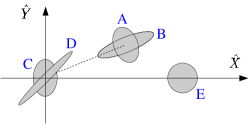
Figure 1: Fluctuation contours of squeezed coherent states (A and B), squeezed vacua (C and D), and a coherent state with real $\alpha$ (E). States A and B have their squeeze phases locked to twice the coherence phase ($\phi=2\theta$), and are therefore respectively amplitude-squeezed ($s<0$) and phase-squeezed ($s>0$) states. State C has $\phi=0$, $s<0$. State D has larger $s$, and $\phi=\pi/2$, so that the tilt is $\pi/4$.

Applying the squeeze operator $\hat{S}$ on a vacuum state produces a single-mode squeezed vacuum, $\left|{\rm sq\_vac(single)}\right.\rangle=\hat{S}\left|{\rm vac}\right.\rangle$, which is another minimum-uncertainty state with distorted variances in the $\hat{X}$-$\hat{Y}$ plane, but the quadrature expectations are now zero (states C, D in Fig. 1). We will be more interested in mixed-mode squeezed vacua,

$$\left|{\rm sq\_vac(mixed)}\right.\rangle=\exp\left[\gamma\hat{c}^{\dagger}_{m}\hat{c}^{\dagger}_{n}-\gamma^{*}\hat{c}_{n}\hat{c}_{m}\right]\left|{\rm vac}\right.\rangle\,,$$

which will be the fate of ${\bf k}\neq{0}$ states in our variational treatment of the non-ideal Bose gas. Squeezing of uncertainty is now seen not in the space of the individual mode quadratures, ($\hat{X}_{m}$, $\hat{Y}_{m}$) or ($\hat{X}_{n}$, $\hat{Y}_{n}$), but in the mixed quadrature variables $\hat{X}=\frac{1}{\sqrt{2}}(\hat{X}_{m}+\hat{X}_{n}$), $\hat{Y}=\frac{1}{\sqrt{2}}(\hat{Y}_{m}+\hat{Y}_{n}$).

After squeezed states became popular in quantum optics in the 1980s, the concept was utilized in the analysis of several condensed matter systems. Squeezed coherent states have been used to treat variationally the “spin-boson” model that arises in connection with dissipative tunneling Leggett et al. (1987), defect tunneling in solids, the polaron problem, etc. Chen et al. (1989); Stolze and Müller (1990); Lo et al. (1994); Dutta and Jayannavar (1994). Squeezed states have also been used for polaritons Artoni and Birman (1991), exciton-phonon systems Sonnek et al. (1995), many-body gluon states Blaschke et al. (1997), bilayer quantum Hall systems Nakajima and Aoki (1997), phonon systems Hu and Nori (1996), and attractive Bose systems on a lattice Sá de Melo (1991).

II.2 Variational wave function and minimization

For a uniform condensate, the macroscopic occupation is in the zero-momentum state, so we will use a coherent occupation of the ${\bf k}=0$ mode only: $\hat{D}=\hat{D}_{0}=\exp\left[\alpha\hat{c}^{\dagger}_{0}-\alpha^{*}\hat{c}_{0}\right]$, with coherence parameter $\alpha=f{\ }e^{i\theta}$. Intuitively, $\alpha$ corresponds to the order parameter for Bose condensation.

We will apply a mixed-mode squeeze operator for each opposite-momenta mode pair. Thus the variational ground state is $\left|{\rm sq1.gr}\right.\rangle=\hat{S}\left|{\rm coh}\right.\rangle=\hat{S}\hat{D}\left|{\rm vac}\right.\rangle$, with

$$\hat{S}=\prod_{{\bf k}}\hat{S}_{{\bf k}}=\prod_{{\bf k}}\exp\left[\frac{1}{2}\left(\gamma_{\bf k}\hat{c}^{\dagger}_{{\bf k}}\hat{c}^{\dagger}_{-{\bf k}}-\gamma_{\bf k}^{*}\hat{c}_{{\bf k}}\hat{c}_{-{\bf k}}\right)\right]\,,$$

$$\gamma_{{\bf k}}+\gamma_{-{\bf k}}=2s_{{\bf k}}e^{i\phi_{{\bf k}}}\,.$$

Note that this automatically includes single-mode squeezing for the condensate (${\bf k}=0$) mode, with squeeze parameter $\gamma_{0}$. Our variational wavefunction for the uniform interacting condensate is thus a squeezed coherent state for the ${\bf k}=0$ mode and a mixed-mode squeezed vacuum for each ${\bf k}{\neq}0$ mode pair.

Minimization of the wavefunction locks the squeeze-parameter phases of each momentum-pair mode to twice the phase of the ${\bf k}=0$ coherence parameter, i.e., $\phi_{\bf k}=2\theta$ for all ${\bf k}$. In the following, we simply start with $\phi_{\bf k}=2\theta$ to avoid typing $(\phi_{{\bf k}}-2\theta)$ arguments.

To determine the variational parameters, we need to minimize the expectation value of the Hamiltonian (1). Expectation values in the variational ground state $\left|{\rm sq1.gr}\right.\rangle$ are calculated using the relations $\hat{D}^{\dagger}\hat{c}_{\bf k}\hat{D}=\hat{c}_{\bf k}+\alpha\delta_{{\bf k},0}$ and $\hat{S}^{\dagger}\hat{c}_{\bf k}\hat{S}=\cosh(s_{{\bf k}})\hat{c}_{{\bf k}}+\sinh(s_{{\bf k}})e^{i\phi_{{\bf k}}}\hat{c}^{\dagger}_{-{\bf k}}$. The required quantities are $\langle\hat{N}_{{\bf k}}\rangle=\langle\hat{c}^{\dagger}_{{\bf k}}\hat{c}_{{\bf k}}\rangle$ and $\langle\hat{H}_{\rm int}\rangle$.

$$\langle\hat{N}_{{\bf k}}\rangle~{}=~{}\sinh^{2}(s_{\bf k})+N_{\rm c}\delta_{{\bf k},0}\,,$$ (2)

and

$$\langle\hat{H}_{\rm int}\rangle~{}=~{}\frac{U}{2V}N_{\rm c}^{2}\\ +~{}\frac{U}{2V}N_{\rm c}\left\{\sum_{\bf q}\cosh(s_{\bf q})\sinh(s_{\bf q})+2\sum_{\bf q}\sinh^{2}(s_{\bf q})\right\}\\ ~{}+~{}\frac{U}{2V}\left\{\left[\sum_{\bf q}\cosh(s_{\bf q})\sinh(s_{\bf q})\right]^{2}+2\left[\sum_{\bf q}\sinh^{2}(s_{\bf q})\right]^{2}\right\}\,.$$

Here we have defined $N_{\rm c}~{}=~{}f^{2}\left[\cosh(2s_{0})+\sinh(2s_{0})\right]$. We can now minimize $\langle{\hat{H}}\rangle=\sum_{{\bf k}}(\epsilon_{{\bf k}}-\mu)\langle{\hat{N}_{{\bf k}}}\rangle+\langle{\hat{H}_{\rm int}}\rangle$ with respect to $N_{\rm c}$ and $s_{{\bf k}}$. This yields

$$\mu~{}=~{}2Un+Um-2Un_{\rm c}$$ (3)

and

$$\sinh(2s_{\bf k})=\frac{-Um}{\sqrt{(\epsilon_{\bf k}-\mu+2Un)^{2}-(Um)^{2}}}\,.$$

Here we have defined $M=\sum_{{\bf q}}\langle\hat{c}^{\dagger}_{\bf q}\hat{c}^{\dagger}_{-{\bf q}}\rangle=N_{\rm c}+\tfrac{1}{2}\sum_{\bf q}\sinh(2s_{\bf q})\,$, and $m=M/V$. We will show in Sec. III.2 that the denominator appearing in $\sinh(2s_{\bf k})$ is the quasiparticle spectrum $E_{{\bf k}}$, and that $\mu-2Un=-Um$. Therefore

$$\sinh(2s_{\bf k})=\frac{-Um}{E_{{\bf k}}}=\frac{-Um}{\sqrt{\epsilon_{{\bf k}}^{2}+2(Um)\epsilon_{{\bf k}}}}\,.$$ (4)

II.3 Expectation values, variances and squeezing

Condensate mode — Expectation values of the bosonic operators are $\langle{\hat{c}_{0}}\rangle=\sqrt{N_{\rm c}}e^{i\theta}$ and $\langle{\hat{c}^{\dagger}_{0}}\rangle=\sqrt{N_{\rm c}}e^{-i\theta}$. It is interesting to contrast this with Bogoliubov’s mean-field prescription, $\langle{\hat{c}_{0}}\rangle=\langle{\hat{c}^{\dagger}_{0}}\rangle=\sqrt{N_{0}}$. Since $N_{0}=N_{\rm c}+\sinh^{2}(s_{0})$, the ${\bf k}=0$ squeezing parameter measures the deviation of our model from mean-field physics. This will be discussed further in Sec. III.3.

Since we have used a squeezed coherent state for the condensate mode, the expectation values and fluctuations of the quadrature operators $\hat{X}_{0}=\frac{1}{2}(\hat{c}_{0}+\hat{c}^{\dagger}_{0})$ and $\hat{Y}_{0}=\frac{1}{2i}(\hat{c}_{0}-\hat{c}^{\dagger}_{0})$ are identical to those for a squeezed coherent state in quantum optics (Sec. II.1, Refs. caves80 ; Loudon and Knight (1987); Loudon (2000)): $\langle{\hat{X}_{0}}\rangle=N_{\rm c}\cos\theta$, $\langle{\hat{Y}_{0}}\rangle=N_{\rm c}\sin\theta$, and

$$\langle{\delta^{2}\hat{X}_{0}}\rangle~{}=~{}\frac{1}{4}\left[e^{2s_{0}}\cos^{2}\theta~{}+~{}e^{-2s_{0}}\sin^{2}\theta\right]\,,$$

$$\langle{\delta^{2}\hat{Y}_{0}}\rangle~{}=~{}\frac{1}{4}\left[e^{2s_{0}}\sin^{2}\theta~{}+~{}e^{-2s_{0}}\cos^{2}\theta\right]\,.$$

The fluctuations along major (minor) axis directions are $\tfrac{1}{2}{e}^{\pm s_{0}}$.

Eq. (4) shows that the squeezing parameter $s_{{\bf k}}$ is negative, becomes large for small ${\bf k}$, and diverges for ${\bf k}=0$. This infrared divergence indicates that $\sinh(2s_{0})$ scales as a positive power of the system size, i.e.,

$$\sinh(2s_{0})=-\gamma_{1}{N}^{\gamma_{2}}\quad\text{and}\quad|s_{0}|\sim\mathcal{O}(\ln{N})\,.$$

The $\gamma$’s can be extracted from finite-size considerations on Eq. (4). Noting that the lowest single-particle state in a box of volume $V$ has energy $\epsilon_{0}=3h^{2}/8\tilde{m}V^{2/3}$, we get $\gamma_{2}=1/3$. The same result can be obtained for a power-law trap. The exact number $\gamma_{1}$ is probably geometry-dependent. However, ignoring factors like 2 and $\pi$ and the difference between $n$ and $n_{\rm c}$, we find $\gamma_{1}\sim\sqrt{n^{1/3}a}$; thus

$$\sinh(2s_{0})\sim-\sqrt{n^{1/3}a}N^{1/3}\,.$$ (5)

upto a factor of order 1. In the true thermodynamic limit, $\sqrt{n^{1/3}a}N^{1/3}\rightarrow\infty$, so the variance profile is squeezed infinitesimally thin in the radial direction. The extension of the variance profile in the phase direction, $\sim\mathcal{O}\left([n^{1/3}a]^{1/4}N^{1/6}\right)$, although diverging, is still infinitesimally small compared to the radial distance ($\sim\sqrt{N}$) of the state from the origin in the quadrature plane. This is symptomatic of the fact that the squeezing has no thermodynamic effects, which we show more explicitly in Sec. III.3.

For finite-size systems, there is significant squeezing only for $n^{1/3}aN^{2/3}\gg{1}$. Note that this is the same condition that decides whether the Thomas-Fermi approximation for a trapped condensate is valid or not.

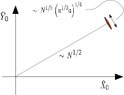
Figure 2: Squeezing of the condensate mode. The variances are very much exaggerated compared to the radial distance from the origin. The displayed variance to radial distance ratio, if drawn to scale, would correspond to $N\sim\mathcal{O}(10^{3})$, in which case a weakly interacting condensate ($an^{1/3}\lesssim{0.1}$) would be barely squeezed.

Nonzero-momentum modes — The ${\bf k}\neq 0$ modes in the wavefunction $\left|{\rm sq1}\right.\rangle$ have the structure of two-mode squeezed vacua. The operators have zero expectation values, $\langle{\hat{c}_{\bf k}}\rangle=\langle{\hat{c}^{\dagger}_{\bf k}}\rangle=0$. There is also no squeezing in quadrature operators defined within a single mode: the usual $\hat{X}_{{\bf k}}$, $\hat{Y}_{{\bf k}}$ have zero expectation values and equal fluctuations.

Squeezing can be seen if one defines the mixed-mode operators

$$\hat{X}_{{\bf k},-{\bf k}}~{}=~{}\frac{1}{\sqrt{2}}(\hat{X}_{{\bf k}}+\hat{X}_{-{\bf k}})~{}=~{}\frac{1}{2\sqrt{2}}(\hat{c}_{\bf k}+\hat{c}_{-{\bf k}}+\hat{c}^{\dagger}_{\bf k}+\hat{c}^{\dagger}_{-{\bf k}})\,,$$

$$\hat{Y}_{{\bf k},-{\bf k}}~{}=~{}\frac{1}{\sqrt{2}}(\hat{Y}_{{\bf k}}+\hat{Y}_{-{\bf k}})~{}=~{}\frac{1}{2\sqrt{2}}(\hat{c}_{\bf k}+\hat{c}_{-{\bf k}}-\hat{c}^{\dagger}_{\bf k}-\hat{c}^{\dagger}_{-{\bf k}})\,.$$

These quadrature operators have zero expectation values and unequal (squeezed) variances $\tfrac{1}{2}\ e^{\pm s_{\bf k}}$.

The formalism of this section also allows us to calculate the occupancies $N_{{\bf k}}=\langle{\hat{c}^{\dagger}_{{\bf k}}\hat{c}_{{\bf k}}}\rangle$ of the non-condensate modes: $N_{{\bf k}}=\sinh^{2}s_{{\bf k}}=\tfrac{1}{2}\left[(\epsilon_{{\bf k}}+Um)/E_{{\bf k}}-1\right]$. This is consistent upto mean field order with standard treatments, e.g., Refs. Glassgold and Sauermann (1969a); Shi and Griffin (1998).

III Symmetry Breaking and Goldstone’s Theorem

We now investigate the symmetry-broken nature of the ground state of the Bose gas. The ground state has a particular phase, thus spontaneously breaking a continuous $U(1)$ symmetry present in the Hamiltonian. Symmetry-broken ground states satisfy a Ward-Takahashi identity reflecting the invariance of the ground-state energy under shifts of the ground state by the symmetry operation in question. According to Goldstone’s theorem, a phase with broken continuous symmetry should have a gapless mode. The Ward identity and gaplessness, both being consequences of the same phenomenon of spontaneous symmetry breaking, are equivalent conditions and can generally be derived from each other. In the case of the Bose gas, the corresponding Ward identity is known as the Hugenholtz-Pines (H-P) theorem Hugenholtz and Pines (1959); Hohenberg and Martin (1964). It is the condition for gaplessness as well as a consequence of the invariance of the ground-state energy under shifts of the $U(1)$ phase. The H-P theorem reads $\mu=\Sigma_{11}(0,0)-\Sigma_{12}(0,0)$, where $\Sigma_{11}({\bf k},\omega)$ and $\Sigma_{12}({\bf k},\omega)$ are the normal and anomalous self-energies.

In Sec. III.1 we use the fact that the Hamiltonian has a $U(1)$ symmetry while the ground state (and hence our variational wavefunction) does not. In Sec. III.2 we calculate the excitation spectrum by constructing a single-quasiparticle wavefunction, and impose the requirement of gaplessness. The two considerations lead to the same condition for the variational parameters, which is comforting in light of Goldstone’s theorem. The condition should be equivalent to the H-P theorem. In Sec. III.3 we compare our Ward identity with the Hartree-Fock-Bogoliubov (mean-field) form of the H-P theorem, and hence evaluate the importance and effects of condensate-mode squeezing, $s_{0}$.

III.1 $U(1)$ symmetry breaking

In our variational wavefunction, the symmetry-broken nature of the ground state appears as the definite phase of the coherence parameter $\alpha=|\alpha|{\ }e^{i\theta}$. A shift of this phase would obviously change the wavefunction, but should not affect the ground-state energy, since the Hamiltonian is $U(1)$-invariant. This requirement will give us the Ward identity for our formalism corresponding to the H-P theorem.

We examine the transformation

$$\alpha\rightarrow\widetilde{\alpha}=\alpha e^{i\lambda}=fe^{i(\theta+\lambda)}\,,\quad\hat{D}\rightarrow\widetilde{\hat{D}}\,,$$

$$\gamma_{{\bf k}}\rightarrow\widetilde{\gamma_{{\bf k}}}=s_{{\bf k}}e^{i(2\theta+2\lambda)}\,,\quad\hat{S}\rightarrow\widetilde{\hat{S}}\,,$$

so that the ground state is shifted, $\left|{\rm sq1.gr}\right.\rangle\rightarrow\left|{\widetilde{\rm sq1.gr}}\right.\rangle~{}=~{}(\widetilde{\hat{S}})^{\dagger}\ (\widetilde{\hat{D}})^{\dagger}\ \left|{\rm vac}\right.\rangle$. We consider infinitesimal $\lambda$, so that $\widetilde{\alpha}\approx\alpha(1+i\lambda)$, and $\widetilde{N_{\rm c}}=N_{\rm c}(1+\lambda^{2})$.

The shift in the thermodynamic potential is

$$\delta\langle\hat{H}\rangle=\langle\left.{\widetilde{\rm sq1.gr}}\right|\hat{H}\left|{\widetilde{\rm sq1.gr}}\right.\rangle-\left<{\rm sq1.gr}|\hat{H}|{\rm sq1.gr}\right>\\ ~{}=~{}\lambda^{2}N_{\rm c}\left\{-\mu+2Un-Un_{\rm c}\right\}\,.$$

We now use the requirement that the grand-canonical energy should not be changed by a shift of the ground state phase, i.e., $\delta\langle{\hat{H}}\rangle=0$. Thus we get

$$\mu=2Un-Un_{\rm c}~{}=~{}2Un-Un_{0}+U\left[\frac{\sinh^{2}(s_{0})}{V}\right]\,\,.$$ (6)

Within the variational formalism, this is our equivalent of the H-P relation.

III.2 Excitation spectrum

We first construct a wavefunction for a Bose-gas ground state with a single-quasiparticle excitation added on top of it:

$$\left|{\rm sq1.ex({\bf k}_{1})}\right.\rangle=\hat{S}\hat{D}\,\hat{c}^{\dagger}_{{\bf k}_{1}}\left|{\rm vac}\right.\rangle\;.$$

The idea is that, since the squeeze operator $\hat{S}$ represents interaction effects in the present formalism, the particle creation operator $\hat{c}_{{\bf k}_{1}}^{\dagger}$ should produce a Bogoliubov quasiparticle when used in conjunction with $\hat{S}$ .

One can evaluate matrix elements of $\hat{N}_{{\bf k}}$ and $\hat{H}_{\rm int}$ in the state $\left|{\rm sq1.ex({\bf k}_{1})}\right.\rangle$ just as was done in the ground state $\left|{\rm sq1.gr}\right.\rangle$. The calculation is lengthier but straightforward. Calculating $\langle{\hat{H}}\rangle$, one now obtains the excitation spectrum as the (grand-canonical) energy of the new state with respect to the ground state.

$$E_{{\bf k}}~{}=~{}\\ \langle\left.{\rm sq1.ex({\bf k}_{1})}\right|\hat{H}\left|{\rm sq1.ex({\bf k}_{1})}\right.\rangle~{}-~{}\langle\left.{\rm sq1.gr}\right|\hat{H}\left|{\rm sq1.gr}\right.\rangle\\ =~{}\cosh(2s_{{\bf k}_{1}})\left[\epsilon_{{\bf k}_{1}}-\mu+2Un\right]+~{}\sinh(2s_{{\bf k}_{1}})\cdot Um\\ ~{}=~{}\left[(\epsilon_{{\bf k}_{1}}-\mu+2Un)^{2}-(Um)^{2}\right]^{1/2}$$

For the spectrum to be gapless, one requires $\mu-2Un=\pm Um$. The positive sign is inconsistent (resulting in $n_{\rm c}=0$). Therefore, we have

$$\mu=2Un-Um$$ (7)

Taken together with Eq. (3), this is indeed identical to the condition (6) obtained from consideration of $U(1)$ symmetry breaking, as expected.

The spectrum we have is thus $E_{{\bf k}}=\sqrt{\epsilon_{{\bf k}}^{2}+2(Un_{\rm c})\epsilon_{{\bf k}}}=\sqrt{\epsilon_{{\bf k}}^{2}+2(Um)\epsilon_{{\bf k}}}$ , which may be contrasted with the Bogoliubov spectrum $E_{{\bf k}}=\sqrt{\epsilon_{{\bf k}}^{2}+2(Un_{0})\epsilon_{{\bf k}}}$ .

III.3 Inferences on condensate mode squeezing

In the thermodynamic limit, $N\rightarrow\infty$, Eq. (5) implies $\sinh^{2}(s_{0})\approx-\tfrac{1}{2}\sinh(2s_{0})\sim\sqrt{n^{1/3}a}N^{1/3}$. Thus, in our Ward identity Eq. (6), the contribution from $s_{o}$ vanishes as $N^{-2/3}$ for macroscopic systems. The effect of condensate-mode squeezing on other thermodynamic quantities and equations similarly vanishes in the $N\rightarrow\infty$, $V\rightarrow\infty$ limit, since $s_{0}$ generally appears as $\sinh^{2}(s_{0})$ or $\sinh(2s_{0})$ in equations involving extensive quantities.

At the mean field Hartree-Fock-Bogoliubov (HFB) level, $\Sigma_{11}=2Un$ and $\Sigma_{12}=Un_{0}$, so that the H-P theorem is $\mu=2Un-Un_{0}$. Comparing with our form $\mu=2Un-n_{\rm c}=2Un-m$, we conclude that the $\hat{S}\hat{D}\left|{\rm vac}\right.\rangle$ formalism reduces to the mean-field HFB results if $N_{0}=N_{\rm c}=M$. Noting from Eq. (2) that

$$N_{0}=\langle{\hat{c}^{\dagger}_{0}\hat{c}_{0}}\rangle=N_{\rm c}+\sinh^{2}(s_{0})\,,$$ (8)

the condition for our formalism to be restricted to mean-field physics is $s_{0}=0$. The ${\bf k}=0$ squeezing parameter is thus a measure of the deviation of the formalism from HFB physics. The point is further emphasized by rewriting Eq. (8) as $\langle{\hat{c}^{\dagger}_{0}\hat{c}_{0}}\rangle=\langle{\hat{c}^{\dagger}_{0}}\rangle\langle{\hat{c}_{0}}\rangle+\sinh^{2}(s_{0})$, which shows that $\sinh^{2}(s_{0})$ acts as a correction to mean-field type decomposition. The argument can be inverted to state that, at mean field level, the weakly interacting $T=0$ Bose gas has no squeezing in the zero-momentum mode. Since $s_{0}=0$ at mean field level, the ${\bf k}=0$ squeezing must come from beyond mean field.

It may seem tempting to try to identify which diagrams contribute to $s_{0}=0$, i.e., to identify contributions to $\Sigma_{12}$ or $\Sigma_{11}$ of the form $U\sqrt{n^{1/3}a}N^{-2/3}$. Note however that these would be non-extensive contributions, which are (not surprisingly) not readily found in the literature.

Note that, in contrast to the ${\bf k}=0$ mode squeezing, the nonzero $\pm{\bf k}$ mixed-mode squeezing in the ${\bf k}{\neq}0$ modes is present at mean field level already.

IV Squeezing in “Fixed-$N$” Excitations

In this Section, we will introduce and study a second variational formulation of the interacting Bose condensate in order to give a more physical interpretation of the squeezing of the nonzero-momentum modes. The formalism will be based on the the bosonic operators introduced by A. E. Ruckenstein in Ref. Ruckenstein (2000).

IV.1 Bosonic fields and excitation Hamiltonian

Ref. Ruckenstein (2000) presents a current algebra approach to formulating a number-conserving description of the Bose condensate. The Hamiltonian is written in terms of density and current operators $\hat{n}({\bf r})=\hat{c}^{\dagger}({\bf r})\hat{c}({\bf r})$ and $\hat{\bf j}=-\tfrac{i}{2m}[\hat{c}^{\dagger}({\bf r}){\bf\nabla}\hat{c}({\bf r})-{\bf\nabla}\hat{c}^{\dagger}({\bf r})\hat{c}({\bf r})]$.

The density fluctuation operator $\hat{\eta}$, defined as $\hat{\eta}({\bf r})=\hat{n}({\bf r})-\langle{\hat{n}({\bf r})}\rangle=\hat{n}({\bf r})-n_{\rm G}({\bf r})$, and the phase operator $\hat{\phi}$, defined by $\hat{\bf j}=\frac{n_{\rm G}({\bf r})}{m}{\bf\nabla}\hat{\phi}({\bf r})$, are canonically conjugate. Defining the linear combinations $\hat{b}({\bf r})$, $\hat{b}^{\dagger}({\bf r})$ with

$$\hat{b}({\bf r})=\frac{1}{2\sqrt{n_{\rm G}({\bf r})}}\left[\hat{\eta}({\bf r})+2in_{\rm G}({\bf r})\hat{\phi}({\bf r})\right]\,,$$

the Hamiltonian in Ruckenstein (2000) takes the form

$$\hat{H}~{}=~{}E_{\rm GS}\left[n_{\rm G}({\bf r})\right]~{}+~{}\hat{H}_{X}\left[n_{\rm G}({\bf r}),\hat{b}({\bf r}),\hat{b}^{\dagger}({\bf r})\right]\,.$$

$E_{\rm GS}$ describes the mean-field ground state, and minimizing this functional gives an equivalent of the Gross-Pitaevskii equation which determines $n_{\rm G}({\bf r})$. In this Article we concentrate on the uniform case, $n_{\rm G}({\bf r})=n_{\rm G}$. We are more interested in the excitation Hamiltonian $\hat{H}_{X}$ which describes the low-lying, large-lengthscale excitations. In momentum space, $\hat{H}_{X}$ reads

$$\hat{H}_{X}~{}=~{}\sum_{{\bf k}{\neq}0}\epsilon_{\bf k}\ \hat{b}^{\dagger}_{\bf k}\hat{b}_{\bf k}\\ ~{}+~{}\tfrac{1}{2}{U}n_{\rm G}\sum_{{\bf k}{\neq}0}\left(\hat{b}^{\dagger}_{\bf k}\hat{b}^{\dagger}_{-{\bf k}}+\hat{b}_{\bf k}\hat{b}_{-{\bf k}}+2\ \hat{b}^{\dagger}_{\bf k}\hat{b}_{\bf k}\right)\,,$$ (9)

modulo an additive constant. Here $\hat{b}_{\bf k}=\int_{\bf r}\hat{b}({\bf r})e^{-i{\bf k}\cdot{\bf r}}$.

The Hamiltonian (9) looks identical to that derived by Bogoliubov. However, the operators in the Bogoliubov Hamiltonian are the original bosonic operators $\hat{c}$, $\hat{c}^{\dagger}$, rather than the peculiar bosons $\hat{b}$, $\hat{b}^{\dagger}$, that we have here. The interpretation is very different; the Bogoliubov picture involves an order parameter and $\pm{\bf k}$ pairs can appear from or disappear into the condensate, while in the fixed-$N$ picture, there is no order parameter. $\hat{H}_{X}$ should not be regarded as a quasiparticle Hamiltonian, but rather as the Hamiltonian describing low-lying density and current oscillations of the system at a fixed total particle number. It is then no surprise that Eq. (9) does not conserve the number of bosons, $\int_{\bf r}\hat{b}^{\dagger}({\bf r})\hat{b}({\bf r})$. Our reason for using this formalism is that the $\hat{b}$ bosons can be interpreted in terms of density fluctuation and phase operators.

Introducing Fourier transforms of the density fluctuation and phase operators, $\hat{\eta}_{\bf k}=\int_{\bf r}\hat{\eta}({\bf r})e^{-i{\bf k}\cdot{\bf r}}$, and $\hat{\phi}_{\bf k}=\int_{\bf r}\hat{\phi}({\bf r})e^{-i{\bf k}\cdot{\bf r}}$. we can express mixed-mode hermitian quadrature operators as

$$\begin{split}\hat{X}_{{\bf k},-{\bf k}}=\frac{1}{4}\left(\hat{b}_{{\bf k}}+\hat{b}_{-{\bf k}}+\hat{b}^{\dagger}_{{\bf k}}+\hat{b}^{\dagger}_{-{\bf k}}\right)=\frac{1}{4n_{\rm G}}\left(\hat{\eta}_{{\bf k}}+\hat{\eta}^{\dagger}_{{\bf k}}\right)\,,\\ \hat{Y}_{{\bf k},-{\bf k}}=\frac{1}{4i}\left(\hat{b}_{{\bf k}}+\hat{b}_{-{\bf k}}-\hat{b}^{\dagger}_{{\bf k}}-\hat{b}^{\dagger}_{-{\bf k}}\right)=\frac{n_{\rm G}}{2}\left(\hat{\phi}_{{\bf k}}+\hat{\phi}^{\dagger}_{{\bf k}}\right)\,.\end{split}$$ (10)

Note that $\hat{X}_{{\bf k},-{\bf k}}$ and $\hat{Y}_{{\bf k},-{\bf k}}$ here are different from the quadrature operators defined in Sec. II.3 because the bosons $\hat{b}$, $\hat{b}^{\dagger}$ have different meanings from $\hat{c}$, $\hat{c}^{\dagger}$.

IV.2 Variational treatment, squeezing

Let us define the reference state $\left|{\rm ref}\right.\rangle$ as the vacuum for the $\hat{b}_{\bf k}$ bosons. We now introduce the following wavefunction as a variational state for the system:

$$\left|{\rm sq2}\right.\rangle=\prod_{{\bf k}{\neq}0}\exp\left[\gamma_{\bf k}\hat{b}^{\dagger}_{{\bf k}}\hat{b}^{\dagger}_{-{\bf k}}-\gamma_{{\bf k}}^{*}\hat{b}_{{\bf k}}\hat{b}_{-{\bf k}}\right]\left|{\rm ref}\right.\rangle=\hat{S}\left|{\rm ref}\right.\rangle\,,$$

with the usual $\gamma_{{\bf k}}+\gamma_{-{\bf k}}=2s_{{\bf k}}\,e^{i\phi_{\bf k}}$.

The state $\left|{\rm ref}\right.\rangle$ itself is determined from the $E_{\rm GS}$ part of the theory. The expectation values in our variational state $\left|{\rm sq2}\right.\rangle$ are $\langle{\hat{b}^{\dagger}_{{\bf k}}\hat{b}_{{\bf k}}}\rangle=\sinh^{2}(s_{\bf k})$ and $\langle{\hat{b}^{\dagger}_{{\bf k}}\hat{b}^{\dagger}_{-{\bf k}}}\rangle=\tfrac{1}{2}\sinh(2s_{\bf k})e^{-i\phi_{\bf k}}$. We will minimize $\langle{H_{X}}\rangle$, not $\langle{H_{X}-\mu\hat{N}}\rangle$. This is because the number of excitations are not conserved, and $\mu$ is determined in the $E_{\rm GS}$ part of the theory. Minimization leads to $\phi_{{\bf k}}=0$, and

$$\sinh(2s_{\bf k})=\frac{-Un_{\rm G}}{\sqrt{\epsilon_{{\bf k}}^{2}+2Un_{\rm G}\epsilon_{{\bf k}}}}\,.$$

One can also calculate the excitation spectrum from this alternate variational procedure. As in Sec. III.2, we can construct the excited state $\left|{\rm sq2.ex({\bf p})}\right.\rangle=\hat{S}{\ }\hat{b}^{\dagger}_{\bf p}\left|{\rm ref}\right.\rangle$. Using expectation values in states $\left|{\rm sq2.gr}\right.\rangle$ and $\left|{\rm sq2.ex({\bf p})}\right.\rangle$, the dispersion relation is found to be $E({\bf p})=\sqrt{\epsilon_{\bf p}^{2}+2\ (Un_{\rm G})\ \epsilon_{\bf p}}$. This is the Bogoliubov spectrum, assuming $n_{\rm G}=n_{0}$. This demonstrates that our new variational formulation captures the physics of the weakly interacting Bose gas at least up to mean field level. We are therefore justified in using the formalism based on the state $\left|{\rm sq2}\right.\rangle$ to draw conclusions about the ${\bf k}{\neq}0$ mixed-mode squeezing.

Just as in Sec. II.3 for the state $\left|{\rm sq1}\right.\rangle$, and in Sec. II.1 for a general two-mode squeezed vacuum, the state $\left|{\rm sq2}\right.\rangle$ displays squeezing in the plane of mixed-mode quadrature operators $\hat{X}_{{\bf k},-{\bf k}}$ and $\hat{Y}_{{\bf k},-{\bf k}}$. However, at this stage the relevant quadrature operators are physically meaningful: $\hat{X}_{{\bf k},-{\bf k}}=\frac{1}{4n_{\rm G}}\left(\hat{\eta}_{{\bf k}}+\hat{\eta}^{\dagger}_{{\bf k}}\right)$ and $\hat{Y}_{{\bf k},-{\bf k}}=\frac{n_{\rm G}}{2}\left(\hat{\phi}_{{\bf k}}+\hat{\phi}^{\dagger}_{{\bf k}}\right)$, as defined in Eq. (10). Since $s_{\bf k}$ is negative, squeezing is along the $\hat{X}_{{\bf k},-{\bf k}}$ direction (Fig. 3). The squeezing is larger for lower momentum.

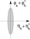
Figure 3: Squeezing of nonzero-momentum modes, in terms of “physical” variables. The variables are Fourier transforms of density fluctuation and phase, in units of $n_{\rm G}$ and $n_{\rm G}^{-1}$ respectively. The density fluctuation variables are squeezed. The squeezing shown here is very moderate, i.e., a large-momentum mode or a condensate with small number of particles.

Thus our study of the alternate variational formulation, in terms of the bosons of the “fixed-$N$” theory Ruckenstein (2000), has allowed us to express a well-known squeezing phenomenon in terms of variables that have the very physical meaning of density fluctuations and phases, albeit in momentum space. This may be regarded as a new formulation of the old idea, attributed to Feynman Feynman (1972, 1953), that in a repulsive Bose condensate, density fluctuations should be suppressed (or in modern language, squeezed).

V Discussion

In summary, we have addressed in detail the issue of squeezing in various modes of the ground state of a uniform condensate, using two different variational wavefunctions.

For squeezing in the condensate mode, we have presented a clear analysis of the scaling of squeeze parameter $s_{0}$ with system size, using our first wavefunction $\left|{\rm sq1}\right.\rangle$, resulting in the scaling relation $e^{2s_{0}}\sim-\sqrt{n^{1/3}a}N^{1/3}$. This leads to the conclusion that while the ground state is indeed squeezed (with the uncertainty profile distortion even diverging for $N\rightarrow\infty$) the squeeze parameter nevertheless has no thermodynamic effects. For finite-size systems, such as condensates in traps, we have identified that the Thomas-Fermi regime ($an^{1/3}\gg N^{-2/3}$) is the interaction regime where one expects to see appreciable squeezing of the ground state.

Our second wavefunction $\left|{\rm sq2}\right.\rangle$ is devised specifically to address the issue of pair squeezing in the non-condensate opposite-momenta mode pairs. Using results from one of the $U(1)$-invariant formulations of the Bose condensate Ruckenstein (2000), we have provided an interpretation of this pair squeezing in terms of variables representing density and phase excitations.

We now make contact with relevant results in the literature. It is worth pointing out that our treatment of gaplessness, where imposing the Hugenholtz-Pines theorem leads to the condition $m=n_{\rm c}$, is actually equivalent to the Popov approximation Popov (1987); Griffin (1996); Shi and Griffin (1998) where anomalous pair correlation functions ($\tilde{m}$ in Ref. Griffin (1996)) are neglected. This is a simple and direct way to implement gaplessness. In Ref. Navez (1998), a more involved procedure for satisfying the Hugenholtz-Pines theorem leads to a macroscopic condensate-mode squeezing. However this contradicts the scaling relationship $e^{2s_{0}}\sim-N^{1/3}$ that we have derived here directly from the minimization of variational parameters. Other scattered previous discussions of squeezing in the condensate mode Solomon et al. (1999); Dunningham et al. (1998); Rogel-Salazar et al. (2002); Glassgold and Sauermann (1969a, b) have not addressed clearly the role of this squeezing in the thermodynamic limit. Finally, concerning the density fluctuation operators borrowed from Ref. Ruckenstein (2000), we note that similar operators have appeared in other fixed-$N$ formulations of the condensate ground state, e.g., in Ref. Gardiner (1997).

We end by pointing out some open problems.

Our results on the condensate-mode squeezing prompts questions about the presence of squeezing in trapped condensates. Study of the quantum state of trapped condensates, either experimentally through quantum state tomography methods or theoretically, is essential for verifying our finite-size scaling relation $e^{2s_{0}}\sim-\sqrt{n^{1/3}a}N^{1/3}$. Refs. Dunningham et al. (1998); Rogel-Salazar et al. (2002) have reported $Q$-function and Wigner function calculations of the condensate quantum state, showing squeezing in a number of cases. However, no systematic analysis of the $N$-dependence or interaction-dependence of the squeezing parameter is available.

Another question related to the quantum state of the condensate mode is the possibility of non-classical features other than squeezing. A whole number of quantum states are studied in quantum optics (Fock, thermal, squeezed Fock, etc.) and it is intriguing to ask if, for example, using a squeezed Fock state instead of a squeezed coherent state for the ${\bf k}=0$ mode would gain us complementary insight. Also, other quantum states might be helpful in exploring ${\bf k}\neq{0}$ physics beyond the mean-field level physics we have extracted here for the non-condensate modes. Inclusion of other quantum-state features might also be fruitful for a variational description of finite-temperature, two-dimensional, or trapped Bose gases.

A real-space variational procedure using wavefunctions of Jastrow form has often been employed to describe interacting Bose condensates Sim et al. (1970); Lee and Wong (1975); Feenberg (1969). A natural question is the relation to our variational description. Presumably, the success of the so-called Bijl-Dingle-Jastrow wavefunction is due to its correctly capturing correlations such as those we have discussed in terms of squeezing. However, it remains unclear how to extract from real-space Jastrow wavefunctions the momentum-space squeezing parameters of the type included in our $\hat{S}\hat{D}$ state $\left|{\rm sq1}\right.\rangle$.

- (1)
- Glauber (1963a) R. J. Glauber, Phys. Rev. 130, 2529 (1963a).
- Glauber (1963b) R. J. Glauber, Phys. Rev. 131, 2766 (1963b).
- Gross (1960) E. P. Gross, Ann. Phys. 9, 292 (1960).
- Cummings and Johnston (1966) F. W. Cummings and J. R. Johnston, Phys. Rev. 151, 105 (1966).
- Langer (1968) J. S. Langer, Phys. Rev. 167, 183 (1968).
- Langer (1969) J. S. Langer, Phys. Rev. 184, 219 (1969).
- Barnett et al. (1996) S. M. Barnett, K. Burnett, and J. A. Vaccarro, J. Res. Natl. Inst. Stand. Technol. 101, 593 (1996).
- (9) J. G. Valatin, in Lectures in Theoretical Physics 1963, University of Colorado Press, Boulder, Colorado, 1964.
- Navez (1998) P. Navez, Mod. Phys. Lett. B 12, 705 (1998).
- Solomon et al. (1999) A. I. Solomon, Y. Feng, and V. Penna, Phys. Rev. B 60, 3044 (1999).
- Dunningham et al. (1998) J. A. Dunningham, M. J. Collett, and D. F. Walls, Phys. Lett. A 245, 49 (1998).
- Rogel-Salazar et al. (2002) J. Rogel-Salazar, S. Choi, G. H. C. New, and K. Burnett, Physics Letters A 299, 476 (2002).
- Valatin and Butler (1958) J. G. Valatin and D. Butler, Nuovo Cimento 10, 37 (1958).
- Glassgold and Sauermann (1969a) A. E. Glassgold and H. Sauermann, Phys. Rev. 182, 262 (1969a).
- Glassgold and Sauermann (1969b) A. E. Glassgold and H. Sauermann, Phys. Rev. 188, 515 (1969b).
- Chernyak et al. (2003) V. Chernyak, S. Choi, and S. Mukamel, Phys. Rev. A 67, 53604 (2003).
- Castin and Dum (1998) Y. Castin and R. Dum, Phys. Rev. A 57, 3008 (1998).
- Lewenstein and You (1996) M. Lewenstein and L. You, Phys. Rev. Lett. 77, 3489 (1996).
- Illuminati et al. (1999) F. Illuminati, P. Navez, and M. Wilkens, J. Phys. B 32, L461 (1999).
- Gardiner (1997) C. W. Gardiner, Phys. Rev. A 56, 1414 (1997).
- Ruckenstein (2000) A. E. Ruckenstein, Found. Phys. 30, 2113 (2000), also available as preprint: cond-mat/0104010.
- Girardeau (1998) M. D. Girardeau, Phys. Rev. A 58, 775 (1998).
- Girardeau and Arnowitt (1959) M. Girardeau and R. Arnowitt, Phys. Rev. 113, 755 (1959).
- Loudon (2000) R. Loudon, The Quantum Theory of Light (Oxford University Press, Oxford, 2000), 3rd ed.
- Hugenholtz and Pines (1959) N. M. Hugenholtz and D. Pines, Phys. Rev. 116, 489 (1959).
- Hohenberg and Martin (1964) P. C. Hohenberg and P. C. Martin, Ann. Phys. 34, 291 (1964).
- Shi and Griffin (1998) H. Shi and A. Griffin, Phys. Rep. 304, 1 (1998).
- Loudon and Knight (1987) R. Loudon and P. Knight, J. Mod. Optics 34, 709 (1987).
- Leggett et al. (1987) A. J. Leggett, S. Chakravarty, A. T. Dorsey, M. P. A. Fisher, A. Garg, and W. Zwerger, Rev. Mod. Phys. 59, 1 (1987).
- Chen et al. (1989) H. Chen, Y. M. Zhang, and X. Wu, Phys. Rev. B 40, 11326 (1989).
- Stolze and Müller (1990) J. Stolze and L. Müller, Phys. Rev. B 42, 6704 (1990).
- Lo et al. (1994) C. F. Lo, E. Manousakis, R. Sollie, and Y. L. Wang, Phys. Rev. B 50, 418 (1994).
- Dutta and Jayannavar (1994) B. Dutta and A. M. Jayannavar, Phys. Rev. B 49, 3604 (1994).
- Artoni and Birman (1991) M. Artoni and J. L. Birman, Phys. Rev. B 44, 3736 (1991).
- Sonnek et al. (1995) M. Sonnek, H. Eiermann, and M. Wagner, Phys. Rev. B 51, 905 (1995).
- Blaschke et al. (1997) D. Blaschke, H.-P. Pave1, V. N. Pervushin, G. Röpke, and M. K. Volkov, Phys. Lett. B 397, 129 (1997).
- Nakajima and Aoki (1997) T. Nakajima and H. Aoki, Phys. Rev. B 56, R15549 (1997).
- Hu and Nori (1996) X. Hu and F. Nori, Phys. Rev. B 53, 2419 (1996).
- Sá de Melo (1991) C. A. R. Sá de Melo, Phys. Rev. B 44, 11911 (1991).
- (41) C. M. Caves, Phys. Rev. D 23, 1693 (1981).
- Feynman (1972) R. P. Feynman, Statistical Mechanics (Addison-Wesley, Reading, Mass., 1972).
- Feynman (1953) R. Feynman, Phys. Rev. 91, 1291 (1953).
- Griffin (1996) A. Griffin, Phy. Rev. B 53, 9341 (1996).
- Popov (1987) Popov, Functional Integrals and Collective Excitations (Cambridge University Press, Cambridge, 1987).
- Gavoret and Nozieres (1964) J. Gavoret and P. Nozieres, Ann. Phys. 28, 349 (1964).
- (47) P. Navez, personal cummunication.
- Sim et al. (1970) H.-K. Sim, C.-W. Woo, and J. R. Buchler, Phys. Rev. Lett. 24, 1094 (1970).
- Lee and Wong (1975) D. K. Lee and K. W. Wong, Phys. Rev. B 11, 4236 (1975).
- Feenberg (1969) E. Feenberg, Theory of Quantum Fluids (Academic Press, N.Y., 1969).