Real-time Monte-Carlo simulations for dissipative tight-binding systemsand time local master equations

Abstract

The numerically exact path integral Monte Carlo approach for the real-time evolution of dissipative quantum systems (PIMC), particularly suited for systems with discrete configuration space (tight-binding systems), is extended to treat spatially continuous and correlated many-body systems. This way, one has to consider generalized tight-binding lattices with either non-equidistant spacing or in higher dimensions, which in turn allows to analyze to what extent Markovian master equations can be applied beyond the usually studied spin-boson type of models.

I Introduction

Quantum Brownian motion is much more involved than its classical analog since in general tractable equations of motion do not exist weiss . Progress can be made in two limiting ranges, namely, in the realm of weak dissipation and in the opposite one of strong friction. In the former case a perturbative treatment has led to a variety of Markovian weak-coupling master equations qmoptics , among them the famous Lindblad lindblad and the Redfield redfield equations. Successful applications include quantum optical systems, decoherence for solid-state based quantum bits and nonadiabatic dynamics in molecular systems, to name but a few. Strong friction has been explored only recently qsmolu1 with a growing amount of research since then qsmolu2 ; qsmolu2a . There, the quantum Smoluchowski equation, a sort of Markovian master equation as well, allows to investigate condensed phase dynamics at lower temperatures e.g. in soft matter and mesoscopic systems qsmolu3 .

A formally exact description of open quantum systems valid for all temperatures and damping strengths is provided by the path integral approach initiated by the work of Feynman and Vernon feynman and developed in detail in the 1980s caldeira ; report ; weiss . The approach has been utilized in numerous applications especially in condensed phase systems, e.g. to reveal the non-exponential decay of low temperature correlation functions, and has further been exploited to consistently derive the Markovian master equations mentioned above qsmolu1 ; karrlein . A real challenge, however, has been to evaluate the formally exact expression for the reduced density matrix in parameter regions where analytical progress and perturbative simplifications are prohibitive. With the increasing complexity of designed and controllable quantum systems on the nanoscale, e.g. for quantum information processing or molecular electronics, the issue of efficient numerical procedures in the real-time domain becomes a very crucial one. Indeed, important achievements have been made in the last decade with the development of advanced path integral Monte-Carlo methods (PIMC) mc1 , the quasi-adiabatic propagator scheme (QUAPI) quapi , stochastic Schrödinger equations strunz , and basis set-methods thoss .

In this context a certain class of systems has been extensively studied, namely, systems with discrete configuration space, also coined tight-binding systems (TBSs). For these systems quantum diffusion takes place on a lattice, where the sites are coupled by tunneling amplitudes, an important case being the restriction to nearest neighbor coupling. The simplest example is the well-known spin-boson model fisher with applications from condensed matter physics to electron transfer reactions. The fundamental role of TBSs follows from the diversity of realizations in physics and chemistry weiss . Transport properties in general multistable systems at sufficiently low temperatures can be described within TBS models leading to relations to the Kondo problem and the Luttinger liquid model. Further, TBSs serve as archetypical models to study quantum phase transitions in correlated systems, as e.g. for Hubbard type of models. Remarkably, even a large class of continuous systems can be mapped exactly onto TBSs by means of duality transformations weiss2 . Based on the path integral representation exact non-Markovian master equations for TBSs weiss have been derived, which provide the starting point for perturbative treatments such as the non-interacting blip approximation (NIBA) and reduce to Markovian ones even for moderate dissipation and low temperatures weiss3 , i.e. far from the limiting ranges addressed above.

The PIMC approach is particularly suited to treat the dissipative real-time evolution of TBSs numerically exactly. While former applications were restricted mainly to two and three state models egger , recently, we substantially improved the approach to apply to more complex systems muehl1 ; muehl2 , such as single charge transfer across long one-dimensional molecular chains including impurities and external driving fields. Moreover, the simulation time range could be extended to cover basically all relevant time scales of the dissipative dynamics. We have been thus in a position to directly access the range of validity of Markovian master equations for TBSs, which in turn are extremely helpful to reveal the relevant physical processes behind the numerical data. The goal of this paper is now twofold: On the one hand we push the PIMC procedure even further and present first results for the dissipative dynamics of spatially continuous and of correlated many-body systems; on the other hand, we give arguments to what extent Markovian master equations can be used in these more involved situations. We will see that this latter question will directly lead us to consider generalized tight-binding lattices with non-equidistant spacing between sites or in higher dimensions.

The article is organized as follows. We start in Sec. II with a brief summary of the path integral representation for open quantum systems and continue in Sec. III to collect the main ideas of the PIMC scheme. Sec. IV deals with known results for non-Markovian and Markovian master equations for TBSs, the applicability of which for one-dimensional chains is illustrated. Then, in Sec. V spatially continuous systems are discussed, before we come to the correlated many-body dynamics in Sec. VI. At the end some conclusions are given.

II Dynamics of dissipative quantum systems

The standard approach weiss for the inclusion of dissipation into a quantum mechanical formulation starts from a system+reservoir model

$$H=H_{S}+H_{R}+H_{I}$$ (1)

with a system part $H_{S}$, an environmental part $H_{R}$, and a system-bath interaction $H_{I}$. The reservoir (heat bath) is mimicked by a quasi-continuum of harmonic oscillators bilinearly coupled to the system:

$$H_{R}+H_{I}=\sum_{\alpha}\left[{P_{\alpha}^{2}\over 2m_{\alpha}}+{1\over 2}m_{\alpha}\omega_{\alpha}^{2}\left(X_{\alpha}+\frac{c_{\alpha}\,\hat{q}}{m_{\alpha}\omega_{\alpha}^{2}}\right)^{2}\right]\;,$$ (2)

where $\hat{q}$ denotes a system operator corresponding to a one-dimensional degree of freedom. Dissipation appears when one considers the reduced dynamics by properly eliminating the bath degrees of freedom, i.e.,

$$\rho(t)={\rm Tr}_{R}\left\{{\rm e}^{-iHt/\hbar}\,W(0)\,{\rm e}^{iHt/\hbar}\right\}$$ (3)

with an initial density matrix $W(0)$ of the total system. It turns out that for the reduced dynamics the environmental parameters enter only via the spectral density

$$J(\omega)=\frac{a^{2}\,\pi}{2\hbar}\sum_{\alpha}\frac{c_{\alpha}^{2}}{m_{\alpha}\omega_{\alpha}}\delta(\omega-\omega_{\alpha})\;,$$ (4)

which effectively becomes a continuous function of $\omega$ for a condensed-phase environment. Note that in the above definition of the spectral density we have included a factor $a^{2}/\hbar$ with $a$ being a proper length scale which is convenient for the treatment of TBSs. The Gaussian statistics of the isolated environment is determined by the complex-valued bath autocorrelation function which for real time $t$ reads

$$L(t) = \frac{a^{2}}{\hbar^{2}}\left\langle\left(\sum_{\alpha}c_{\alpha}X_{\alpha}(t)\right)\left(\sum_{\alpha}c_{\alpha}X_{\alpha}(0)\right)\right\rangle_{\beta}$$ (5)

$$= {1\over\pi}\int_{0}^{\infty}\!d\omega\,J(\omega){\cosh[\omega(\hbar\beta/2-it)]\over\sinh(\hbar\beta\omega/2)}\;,$$

where $\beta=1/k_{B}T$.

In the sequel we focus on systems evolving in a discretized configuration space with respect to the pointer variable $q$ and thus consider the population $P(q_{f},t)$ of a “lattice site” $q_{f}$ determined by the diagonal part of the reduced density matrix, i.e.,

$$P(q_{f},t)={\rm Tr}\left\{|q_{f}\rangle\!\langle q_{f}|\,\rho(t)\right\}\;,$$ (6)

which is normalized $\int dqP(q,t)=1$. Accordingly, the initial density matrix of the total compound $W(0)$ in (3) is taken to be

$$W(0)=Z_{R}^{-1}|q_{i}\rangle\!\langle q_{i}|\,e^{-\beta(H_{R}-q_{i}\mu{\cal E})}\;$$ (7)

with the partition function of the isolated reservoir $Z_{R}$. The bath is equilibrated according to a localized initial state of the system on a lattice site $q_{i}$, where $\mu{\cal E}=\sum_{\alpha}c_{\alpha}X_{\alpha}$ so that e.g. for electron transfer in a polar environment, $\mu$ is the electronic dipol moment and ${\cal E}$ the collective dipol moment of the bath. Generalizations to delocalized initial states for the system are straightforward report .

The path integral representation provides a formally exact expression for the reduced dynamics and is thus the starting point for a numerically exact Monte-Carlo (MC) scheme. Along the lines sketched above, the bath degrees of freedom are eliminated exactly to arrive at the reduced dynamics. As shown in Ref. weiss , one thus obtains for Eq. (6)

$$P_{s_{f},s_{i}}(t)=\oint\!{\cal D}\tilde{s}\;\delta_{\tilde{s}(t),s_{f}}\exp\left\{{i\over\hbar}S_{S}[\tilde{s}]-\Phi[\tilde{s}]\right\}\;.$$ (8)

Here the path integration runs over closed paths $\tilde{s}(\tilde{t})$ connecting $\tilde{s}(0)=s_{i}$ with $\tilde{s}(t)=s_{f}$ along the real-time contour $\tilde{t}\in 0\rightarrow t\rightarrow 0$, which combines the forward and backward paths $s(t^{\prime})$ and $s^{\prime}(t^{\prime})$, respectively. Furthermore, $S_{S}[s]$ denotes the action of the free system. The influence of the traced-out bath is completely encoded in the Feynman-Vernon influence functional $\Phi[s]$ feynman

$$\Phi[q,q^{\prime}] = \int_{0}^{t}\!dt^{\prime}\!\int_{0}^{t^{\prime}}\!dt^{\prime\prime}[q(t^{\prime})-q^{\prime}(t^{\prime})]\ [{L}(t^{\prime}-t^{\prime\prime})q(t^{\prime\prime})$$ (9)

$$\qquad{}-{L}^{\ast}(t^{\prime}-t^{\prime\prime})q^{\prime}(t^{\prime\prime})]$$

$${}+i{{\hat{\mu}}\over 2}\int_{0}^{t}\!dt^{\prime}[q^{2}(t^{\prime})-q^{\prime 2}(t^{\prime})]\;,$$

where

$${\hat{\mu}}={2\over\pi}\int_{0}^{\infty}\!d\omega{J(\omega)\over\omega}\;.$$ (10)

The influence functional introduces long-ranged nonlocal interactions among the system paths so that in general an explicit evaluation of the remaining path integral in Eq. (8) is possible only numerically. In this situation the PIMC method has been proven as a very promising approach to obtain numerically exact results even in regions of parameter space where other approximate methods fail.

III PIMC simulation method

A prerequisite for an efficient numerical algorithm is an appropriate discretization of time and configuration space. The latter one is intrinsically given for multistable systems in the tight binding limit, where the relevant states are strongly localized in position, only very weakly coupled by tunneling, and energetically well separated from the rest of the spectrum. For spatially continuous systems supporting delocalized states the situation is less obvious, but in case of a discrete energy spectrum a mapping onto a generalized tight-binding lattice applies as well for lower temperatures quapi ; grifoni . In any case, the configuration space variable can then be written as $q(t)=a\cdot s(t)$ with a typical length scale $a$ and a dimensionless variable $s(t)\in\{q_{1},\ldots,q_{d}\}$ with $-S=q_{1}<q_{2}<\cdots<q_{d}=S$ according to a $d$-level system ($d$LS). Hence, the system Hamiltonian reads

$$H_{d{\rm LS}}=\hbar E_{z}-\hbar S_{x}\;,$$ (11)

where $E_{z}$ describes the energetic distribution of the sites according to $E_{z}|q_{\mu}\rangle=\epsilon_{\mu}|q_{\mu}\rangle$ and $S_{x}$ the couplings between them $\Delta_{\mu\nu}=\langle q_{\mu}|S_{x}|q_{\nu}\rangle,\mu\neq\nu$. In particular, in case of $q_{\mu+1}-q_{\mu}=1$ and nearest neighbor coupling only one recovers a $(2S+1)$-spin-boson model.

For the discretization in time, the time axis is sliced via $r$ uniformly spaced points with discretization steps $\tau=t/r$. The path integral in Eq. (8) then becomes

$$P_{s_{f},s_{i}}(t)=\sum_{\{s_{j}\}}\delta_{s_{r+1},s_{f}}\rho[\{s_{j}\}]$$ (12)

with

$$\rho[\{s_{j}\}]=\left[\prod_{k=1}^{2r}K(s_{k},s_{k+1})\right]e^{-\Phi[\{s_{j}\}]}\;.$$ (13)

The sum runs over all realizations of the discretized spin path $\{s_{j}\}=\{s_{1}\equiv s_{i},s_{2},\dots,s_{2r},s_{2r+1}\equiv s_{i}\}$, and $K(s_{j},s_{j+1})$ denotes the coordinate representation of the free $d$LS propagation over the time interval $\tau$, i.e.,

$$K(s,s^{\prime},\tau)=\langle s|\exp(-i\tau H_{d\rm LS}/\hbar)|s^{\prime}\rangle\;.$$ (14)

This propagator of the $d$LS Hamiltonian can be obtained from the eigenstates

$$H_{d\rm LS}|\phi_{\alpha}\rangle=E_{\alpha}|\phi_{\alpha}\rangle\,,\quad\alpha=1,\ldots,d$$ (15)

as

$$K(s,s^{\prime},\tau)=\sum_{\alpha=1}^{d}\langle s|\phi_{\alpha}\rangle\langle\phi_{\alpha}|s^{\prime}\rangle\ {\rm e}^{-i\tau E_{\alpha}/\hbar}\;,$$ (16)

which can be easily computed numerically once the $d$LS’s parameters are specified.

To arrive at a discretized form (in time) of the influence functional (9), the sum and difference coordinates

$$\eta(t^{\prime})\equiv s(t^{\prime})+s^{\prime}(t^{\prime})\;,\qquad\xi(t)\equiv s(t^{\prime})-s^{\prime}(t^{\prime})$$ (17)

are introduced, which read $\eta(t^{\prime})=\eta_{j}$ ($\xi(t^{\prime})=\xi_{j}$) for $t^{\prime}\in[(j-1)\tau-\tau/2,(j-1)\tau+\tau/2]$ in their discretized form. The sum paths are also considered as “quasi-classical”, while the difference paths capture quantum fluctuations weiss . Equation (9) finally can be written as

$$\Phi[s_{i},\eta,\xi] = i\sum_{j=2}^{r}\xi_{j}\hat{X}^{(s_{i})}_{j}$$

$${}+\sum_{j\geq k=2}^{r}\xi_{j}(iX_{j-k}\eta_{k}+\Lambda_{j-k}\xi_{k})$$

where the kernels $\hat{X}^{(s_{i})}_{j}$, $X_{j-k}$, and $\Lambda_{j-k}$ follow from discretizing the twice integrated bath autocorrelation function $Q(t)$ defined by $\ddot{Q}(t)=L(t)$, $Q(0)=0$ with $\dot{Q}(0)=i\hat{\mu}/2$. In the sequel we consider a spectral density of the form

$$J(\omega)=2\pi\alpha\omega{\rm e}^{-\omega/\omega_{c}}\;,$$ (19)

which is equivalent to ohmic damping with a cut-off frequency $\omega_{c}$. In this case $Q(t)$ can be calculated analytically and one obtains

$$Q(t)=2\alpha\Bigg{[}\ln(1+i\omega_{c}t)-\ln\frac{\Gamma(\Omega+it/\hbar\beta)\Gamma(\Omega-it/\hbar\beta)}{\Gamma^{2}(\Omega)}\Bigg{]}$$ (20)

with $\Omega=1+1/(\hbar\beta\omega_{c})$ and the Gamma function $\Gamma(z)$.

Equations (12), (13) and (III) constitute a discretized form of the populations (6) and thus provide a starting point for PIMC simulations. As it is well-known this method is handicapped by the dynamical sign problem sign-problem . It originates from quantum interferences between different system paths $\{s_{j}\}$, causing a small signal-to-noise ratio of the stochastic averaging procedure.

One approach to deal with this problem is based on the observation that the quasi-classical paths $\{\eta_{j}\}$ in Eq. (III) can be integrated out as a series of $r-1$ matrix multiplications egger3 . This reduces the degrees of freedom from the $2r-1$ variables $\{\eta_{2\leq j\leq r+1},\xi_{2\leq j\leq r}\}$ to the $r-1$ quantum variables $\{\xi_{2\leq j\leq r}\}$ and therefore significantly improves the numerical stability of the corresponding MC simulations. While this technique, which in fact is yet another example of a blocking approach blocking , works greatly for dissipative two- and three-state systems egger , however, the increasing size of the corresponding matrices with the number of electronic sites turns these multiplications into a quite time consuming task. Since they have to be performed for every single update of the MC trajectory, the investigation of larger systems again requires exceptionally long CPU times.

Nevertheless, this severe computational bottleneck can be profoundly alleviated on physical grounds muehl1 ; muehl2 . Upon closer inspection one finds that the possibility of rewriting the integration over the quasi-classical coordinates in terms of simple matrix multiplications is due to the fact that the real-valued part of the bath autocorrelation function (5) governs only the quantum coordinates but not the quasi-classical ones. This real-valued part, which eventually leads to a damping out of quantum coherences, introduces a non-local self-coupling among the quantum coordinates and is thus directly related to retardation effects, a main complication for treating dissipative quantum systems. Accordingly, the retardation effects influence the evolution of the quasi-classical coordinates contained in the imaginary part of the influence functional to a significantly weaker extend than that of the quantum coordinates. Neglecting them while generating the MC trajectories leads to an only minor impairment of the sampling statistics, but causes an almost complete decoupling between quantum and quasi-classical coordinates. This in turn allows for an enormous speed-up of the matrix multiplications. Accordingly, the sampling process could so far be accelerated by a factor of approximately 100 with respect to the original approach egger (for further details, we refer to Refs. muehl1 ; muehl2 ), thus opening the door to treat the reduced dynamics of much larger and even many-body systems over sufficiently long times.

IV Time-local master equations

From the exact expression (8) for the reduced density simplifications can be derived in certain limits in terms of time-local master equations. In the context discussed here, these are of crucial importance, mainly since (i) master equations allow to study ranges in parameter space where the Monte Carlo sampling is rather expensive, e.g. for very weak or very strong friction, and (ii) they provide a basis to access the physical processes underlying the numerical data also by means of analytical techniques.

In the weak friction limit one imposes that the level broadening due to friction is much smaller than $k_{\rm B}T$ and the typical level separation. It is thus natural to work in the basis spanned by the energy eigenstates of $H_{S}$ and to treat the coupling $H_{I}$ perturbatively. With increasing coupling, however, the environment drives the system to its pointer basis in which the system-bath coupling operator $q$ is diagonal. As we have seen above in Sec. II, in this basis the path integral formulation allows for a non-perturbative elimination of the reservoir degrees of freedom. In case that friction is very strong and thus level broadening much larger than level spacing and temperature, a master equation complementary to the weak friction range, the quantum Smoluchowski equation, is again available qsmolu1 ; lehle .

What’s about the intermediate regime? For TBSs discussed here, substantial findings have been gained in the past decade weiss . Namely, it was shown that an exact retarded master equation exists, i.e.,

$$\frac{dP_{\mu_{f},\mu_{i}}(t)}{dt}=\sum_{\nu=1}^{d}\int_{0}^{t}dt^{\prime}\ \hat{\Gamma}_{\mu_{f}\nu}(t-t^{\prime})\,P_{\nu,\mu_{i}}(t^{\prime})\,,$$ (21)

where the kernels obey $\hat{\Gamma}_{\mu\mu}=-\sum_{\nu\neq\mu}\hat{\Gamma}_{\mu\nu}$. Basically they represent a power series in the couplings $\Delta_{\mu\nu}$ with corresponding spin-path integrals. To make the latter tractable, one applies the NIBA fisher or its generalization, the non-interacting cluster approximation (NICA) weiss , which has been shown to be accurate in a variety of parameter ranges. For instance, in case of an ohmic spectral density with a high frequency cut-off, it captures quantum coherence as well as pure relaxation dynamics. The corresponding kernels $\tilde{\Gamma}_{\mu\nu}$ read in lowest order in the intersite couplings

$$\tilde{\Gamma}_{\mu\nu}^{(2)}(t) = 2\Delta_{\mu\nu}^{2}\ \exp\left[-(q_{\mu}-q_{\nu})^{2}\,Q^{\prime}(t)\right]$$ (22)

$$\cos\left[(\epsilon_{\mu}-\epsilon_{\nu})t+(q_{\mu}-q_{\nu})^{2}\,Q^{\prime\prime}(t)\right]\,$$

with $Q^{\prime}={\rm Re}Q(t)$ and $Q^{\prime\prime}={\rm Im}Q(t)$. The practical use of (21) is limited though due to the retardation.

Now, for sufficiently strong dissipation and fast enough bath modes the kernel falls off on a time scale much shorter than the time scale on which the relevant reduced dynamics occurs so that we may set in (21) $P_{\nu,\mu_{i}}(t^{\prime})\approx P_{\nu,\mu_{i}}(t)$ and

$$\Gamma_{\mu\nu}=\int_{0}^{\infty}dt\,\tilde{\Gamma}_{\mu\nu}(t)\,.$$ (23)

Accordingly, (21) reduces to a simple Markovian rate equation

$$\dot{{\mathbf{P}}}(t)=A\,{\mathbf{P}}(t)\;,$$ (24)

with a rate matrix $A$ consisting of the individual rates $\Gamma_{\mu\nu}$. For nearest neighbor coupling, the golden rule rates $\Gamma_{\mu\nu}^{(2)}$ describe a sequential hopping process, while all higher order contributions to $\Gamma_{\mu\nu}$ capture long-range hopping termed superexchange. Note that in contrast to weak coupling master equations as e.g. the Redfield equations, (21) and (24) together with the corresponding transition rates apply also to the range of moderate to strong bath coupling and very low temperatures.

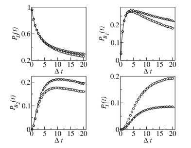
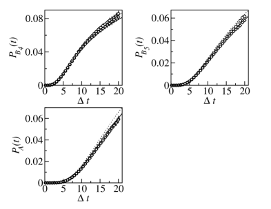
Figure 1: Populations along a molecular chain with $d=7$ sites obtained from PIMC simulations (symbols) and from the local master equation approach (lines). Donor (D) and acceptor (A) are connected by a bridge with an impurity (I) at its center. The impurity has an onsite energy relative to D/A of $\epsilon_{I}/\Delta=+5$ (PIMC: diamonds; master equation: solid lines) and $\epsilon_{I}/\Delta=-5$ (PIMC: circles; master equation: diamonds). Other parameters are $\alpha=0.1,\Delta\hbar\beta=0.1,\omega_{c}/\Delta=5$, see text for details.

As an explicit example of (24) we consider a one-dimensional tight-binding lattice with $d=7$ sites, spacing 1, and constant nearest neighbor coupling corresponding to a spin-3-boson system (for details see muehl2 ). This model can be seen as a simple realization of electron transfer along a molecular chain subject to a dissipative environment jortner ; muehl1 . Initially, the charge is localized at the donor site $s_{i}=q_{1}=-3$ and $P_{s_{f},-S}(t)$ monitors the dynamics towards the acceptor at $q_{7}=3$. Specifically, donor and acceptor are linked by a bridge with an impurity at its center. Donor/acceptor have vanishing onsite energy, the bridge sites are elevated by $\epsilon_{B}/\Delta=2.5$, and the impurity site has $\epsilon_{I}/\Delta=\pm 5$. As seen in fig. 1 the exact PIMC data are very accurately described by the time-local master equation (24) despite the fact that all parameters are chosen such that one is close to a coherent/incoherent transition (for the given values of $\omega_{c}$ and $\alpha$ coherences appear at inverse temperatures $\hbar\beta\Delta\approx 0.3$ and larger) and $\omega_{c}/\Delta=5$ is far from the scaling limit.

V Dynamics of spatially continuous systems

In order to go beyond the spin-boson type of models (one-dimensional tight binding lattice, equidistant spacing, constant nearest coupling), we start by presenting an approach to capture the dynamics of spatially continuous systems within the PIMC procedure outlined above. It turns out that this method applies to systems with a discrete energy spectrum. The basic idea is simple: For sufficiently low temperatures only the lowest lying states of the isolated system can be assumed to take part in the dynamics; thus, the full Hilbert space $H_{S}$ can effectively be truncated to a subspace $H_{S}^{(N)}$ spanned by the $N$ lowest lying eigenstates. One then has to find a proper basis in this subspace, obtained by a unitary transformation from the eigenstate basis, in which a stochastic sampling of the path integrals (8) can be performed.

This sort of reduction is not new. In fact, the spin-boson model can be seen as originating from a double well potential, where only the two lowest lying states are taken into account. Of course, the goal here is to go beyond: We want to capture the dissipative dynamics from very low up to moderate temperatures. For very high temperatures semi-classical or classical methods apply anyway. Further, we are interested in the regime of moderate friction, where neither of the known approximate formulations work so that a numerical treatment has to start from the exact reduced dynamics (8). The proper basis for the sampling in the restricted Hilbert space is then the basis that diagonalizes the operator $\hat{q}$ in $H_{S}^{(N)}$. This idea to treat spatially continuous systems has been first applied in the numerical QUAPI approach quapi and has been recently analyzed in grifoni to derive a generalized master equation of the type given above (21). Hence, we sketch here only the central results briefly and refer to these previous works for further details.

In the $N$-dimensional subspace $H_{S}^{(N)}$ the pointer basis is defined as

$$\hat{q}|q_{\nu}\rangle=aq_{\nu}\,|q_{\nu}\rangle\ ,\ \nu=1,\ldots,N$$ (25)

and obtained from the eigenstate basis $\{|n\rangle\}$ by diagonalizing a matrix with entries $\langle n|\hat{q}|m\rangle$, $n,m=1,\ldots,N$. Its eigenvalues provide the dimensionless $q_{\nu}$, while the eigenvectors are given as $|q_{\nu}\rangle=\sum b_{\nu n}|n\rangle$. The basis set $\{|q_{\nu}\rangle\}$ is also known as the DVR-basis (Discrete Value Representation). By representing the Hamiltonian in this DVR-basis, one obtains “onsite energies” $\hbar\epsilon_{\nu}=\langle q_{\nu}|H_{S}|q_{\nu}\rangle$ and “intersite-couplings” $\Delta_{\nu\mu}=\langle q_{\nu}|H_{S}|q_{\mu}\rangle/\hbar$. The original system is thus mapped onto a generalized $N$-dimensional tight-binding lattice with non-equidistant sites at $q_{\nu},\nu=1,\ldots,N$ and non-nearest neighbor couplings $\Delta_{\nu\mu}$. Now, to implement this TBS into the PIMC algorithm, one has to take into account the non-equidistant lattice by re-defining the $\xi_{j}$ and $\eta_{j}$ variables properly.

A rough estimate for the validity of the truncation procedure to the lowest $N$ eigenstates of the isolated system is given by the conditions that (i) the level broadening due to friction is of the same order as the level spacing or smaller and that (ii) the temperature is sufficiently low $N\hbar\beta\omega_{0}\gg 1$. While the second condition is obvious, the first one originates from the fact that for very strong friction the system tends to the classical limit again, see qsmolu1 .

By way of example, we consider in the sequel a harmonic oscillator with mass $M$ and frequency $\omega_{0}$, so that the typical length scale is $a\equiv q_{0}=\sqrt{\hbar/M\omega_{0}}$. While a detailed account of the implementation into the PIMC algorithm and results of simulations for specific observables, particularly in comparison with analytical results, will be given elsewhere, here, our main interest is to explicitly show that apart from the conditions for the applicability of time local master equations known for spin-boson models, the treatment of continuous systems via the described mapping comes with an additional complication. Formally, this issue has also been addressed recently in grifoni . Here, we directly compare numerically exact PIMC data with results from the simplified master equation. For this purpose the initial state is chosen as one of the DVR-states which suffices to study the time evolution of the populations on the sites $q_{\nu}$.

Figure 2: DVR-site populations for a harmonic oscillator with $N=5$ eigenstates obtained from PIMC simulations (symbols) and a master equation approach (solid lines). Top left: $P_{1}$ (diamonds) and $P_{5}$ (circles), top right: $P_{2}$ (diamonds) and $P_{4}$ (circles), bottom left: $P_{3}$, bottom right: average position, see text for details.

Figure 3: Same as in fig. (2) but for $N=7$. Top left: $P_{1}$ (diamonds) and $P_{7}$ (circles), top right: $P_{2}$ (diamonds) and $P_{6}$ (circles), middle left: $P_{3}$ (diamonds) and $P_{5}$ (circles), middle left: $P_{4}$, bottom: average position, see text for details.

Results for $N=5$ and $N=7$ are depicted in figs. 2, 3 for a bath with $\omega_{c}/\omega_{0}=5$, $\alpha=0.2$, and $\hbar\beta\omega_{0}=0.2$. For this parameter set we have shown recently muehl1 ; muehl2 that time local master equations capture the exact dynamics of linear chains rather accurate even though one is close to an incoherent/coherent transition for the reduced dynamics. The same is true here for $N=5$, where we used (24) together with the hopping rates (23). In contrast, for $N=7$ deviations appear in the short to intermediate time regime. For times of the order of $1/\omega_{c}$ and shorter ($\omega_{0}t\leq 0.2$), these are caused by adiabatic effects in the bath well-known from the dynamics in ordinary tight binding lattices. In the intermediate time range, however, where for certain populations pronounced maxima occur, deviations must be ascribed a specific property related to the mapping onto a tight binding lattice with non-equidistant spacing. As mentioned above, this mapping requires a re-definition of the $\xi$ and $\eta$ variables, originally defined for a tight binding lattice with equidistant spacing of length $a$.

Qualitatively, the situation is the following: Since the variance of the $N$th eigenstate is roughly $(\Delta q^{2})_{N}\approx Nq_{0}^{2}$, the box in position space covered by $N$ states has a typical width $L\approx 2\sqrt{N}q_{0}$. The mean spacing between adjacent lattice sites is thus $a_{\rm eff}\approx L/N=2q_{0}/\sqrt{N}$. Hence, compared to a lattice with equidistant spacing of length $a=q_{0}$, the re-definition of the $\xi$ and $\eta$ variables in the influence functional (III) comes with an additional factor of the order $(2/\sqrt{N})^{2}$, which basically renormalizes the damping kernel. Consequently, for fixed bath parameters and increasing $N$, the effective coupling constant between bath and discrete system is not constant, but decreases as $4\alpha/N$. The system is thus driven into the range of weak coupling to the bath grifoni , where retardation effects due to quantum coherences become more substantial. Hence, the limit to a spatially continuous system $N\to\infty$ is non-trivial and must be performed by keeping $\alpha/N$ constant. Specifically, by comparing the spectral density (19) with the one usually introduced for spatially continuous systems weiss , one finds

$$\frac{4\alpha\pi}{{N}}\approx\frac{\gamma}{2\omega_{0}}\ ,$$ (26)

where $\gamma$ denotes the macroscopic damping constant appearing in the classical Langevin equation. Note that the above relation cannot be seen as a strict equality since the spacing between adjacent DVR-sites varies slightly and is typically smaller deep inside the potential well. The value $\alpha=0.2$ chosen above corresponds for $N=5$ to $\gamma/\omega_{0}\approx 1$ and for $N=7$ to $\gamma/\omega_{0}\approx 0.7$. Now, a rough estimate for the validity of time local master equations can be gained by assuming that the exponential in (22) must fall off on a time scale sufficiently shorter than that of the dynamics of $P_{\mu}(t)$. For moderate and low temperatures, this leads to $1/(\omega_{c}\sqrt{\alpha/N}){\textstyle{\lower 2.0pt\hbox{$<$}\atop\raise 1.0pt\hbox{$\sim$}}}1/\omega_{0}$ and thus $N{\textstyle{\lower 2.0pt\hbox{$<$}\atop\raise 1.0pt\hbox{$\sim$}}}\alpha(\omega_{c}/\omega_{0})^{2}$. In accordance with this relation, the PIMC data presented in fig. 2, 3 for $N=5$ can still be captured quantitatively by (24), while for $N=7$ only a qualitative agreement can be seen. To perform the continuum limit is thus not an easy task and certainly deserves further research.

VI Correlated two-particle dynamics

The dissipative real-time evolution of interacting many body systems has been left basically untouched so far. In certain limits, e.g. for very strong repulsive interactions, results could be derived from a simple hopping model petrov , but the intimate interplay between direct interaction, interaction mediated by the environment and dissipation has not been accessible. Here, for the first time we present PIMC results for the dynamics of two interacting particles along the lines described above. As in the previous section, in the sequel the formulation is outlined only briefly and we focus on conceptual properties related to time-local master equations. Further, we consider the case of indistinguishable particles, called charges henceforth, so that the quantum nature of the particle statistics matters. Physically, the situation refers to interacting spinless fermions or interacting bosons.

The free system is taken as a tight-binding lattice with spacing 1 and nearest neighbor coupling, where the two charges can be placed on $d=2S+1$ sites. Accordingly, the two-charge Hamilton operator reads

$$H_{d{\rm LS}}^{(2)}=\hbar\left\{{E}_{z}-[{S}_{x}^{(a)}+{S}_{x}^{(b)}]+{U}\right\}$$ (27)

where ${E}_{z}$ and ${S}_{x}^{(j)},j=a,b$ are straightforward generalizations of the corresponding operators introduced above for the single particle case, while ${U}$ describes a site dependent Coulomb interaction specified below. The coupling to the bath is determined by the total dipol-moment of the system and thus follows directly from (2):

$$H = H_{d{\rm LS}}^{(2)}+\sum_{\alpha}\left\{{P_{\alpha}^{2}\over 2m_{\alpha}}+\frac{1}{2m_{\alpha}\omega_{\alpha}^{2}}\right.$$ (28)

$$\hskip 28.45274pt\left.\times\left[X_{\alpha}-\frac{c_{\alpha}a}{m_{\alpha}\omega_{\alpha}^{2}}\left({S}_{z}^{(a)}+{S}_{z}^{(b)}\right)\right]^{2}\right\}$$

with ${S}_{z}^{(j)}|s^{(j)}\rangle=s^{(j)}\,|s^{(j)}\rangle,j=a,b$.

Since the two charges are indistinguishable it is convenient for the PIMC simulation to work not in the single particle product basis, but rather in the basis of the many body states. For this purpose we introduce

$$\{|s^{(a)}\rangle|s^{(b)}\rangle\}\longrightarrow\{|s,\hat{s}\rangle\}$$ (29)

with $s\leq\hat{s}$. The advantage of this representation is that the $d(d+1)/2$ states $\{|s,\hat{s}\rangle\}$ are orthogonal in contrast to the original ones. Accordingly, $H_{d{\rm LS}}^{(2)}$ takes the form

$$H_{d{\rm LS}}^{(2)}=\hbar\left[{E}_{z}-{S}_{x}+{U}\right]$$ (30)

where now

$${E}_{z}|s,\hat{s}\rangle = (\epsilon_{s}+\epsilon_{\hat{s}})|s,\hat{s}\rangle$$

$${S}_{x}|s,\hat{s}\rangle = \delta_{s=\hat{s}}(\Delta_{s-1}|s-1,s\rangle+\Delta_{s}|s,s+1\rangle)$$

$${}+\delta_{s\neq\hat{s}}(\Delta_{s-1}|s-1,\hat{s}\rangle+\Delta_{\hat{s}}|s,\hat{s}+1\rangle$$

$${}+\Delta_{s}|s+1,\hat{s}\rangle+\Delta_{\hat{s}-1}|s,\hat{s}-1\rangle)$$

$${U}|s,\hat{s}\rangle = \frac{1}{2}(u_{s,\hat{s}}+u_{\hat{s},s})|s,\hat{s}\rangle\,.$$ (31)

For an onsite Coulomb energy this model is identical to a dissipative Hubbard model with two charges. Note, however, that for the PIMC simulations a non-local interaction can easily be taken into account.

Now, as seen above, the free system dynamics enters in the discretized path integral formulation only through its short time propagator which is conveniently represented in the energy eigenbasis of $H_{d{\rm LS}}^{(2)}$ in (30), see (16). Further, since in (28) the two charges interact with the bath only via the sum $S_{z}^{(a)}+S_{z}^{(b)}$ the corresponding change to the many body basis in the influence functional is straightforward. It amounts to introduce discretized sum and difference paths according to

$$\eta_{j}\equiv s_{j}+s^{\prime}_{j}\;, \xi_{j}\equiv s_{j}-s^{\prime}_{j}\;,$$

$$\hat{\eta}_{j}\equiv\hat{s}_{j}+\hat{s}^{\prime}_{j}\;, \hat{\xi}_{j}\equiv\hat{s}_{j}-\hat{s}^{\prime}_{j}\,$$ (32)

such that the influence functional depends only on $\eta(t^{\prime})+\hat{\eta}(t^{\prime})$ and $\xi(t^{\prime})+\hat{\xi}(t^{\prime})$.

Figure 4: Mapping of a two charge system moving in a one-dimensional tight binding lattice onto a one particle system diffusing on a two-dimensional triangular lattice.

In principle, we could now start to implement the above representation into a PIMC algorithm. However, before doing so we go one step further and exploit the following crucial property: The dissipative dynamics of two indistinguishable charges on a one-dimensional lattice with $d$ sites is equivalent to the dissipative dynamics of a single particle on a two-dimensional triangular lattice with $d(d+1)/2$ sites. To see this, one realizes that the coupling to the bath $({S}_{z}^{(a)}+{S}_{z}^{(b)})\,\mu{\cal E}$ with $\mu{\cal E}$ as in (7) can be written as $\vec{\mu}\cdot\vec{\cal E}$ with the vector operators $\vec{\mu}=(\mu\,{S}_{z}^{(a)},\mu\,{S}_{z}^{(b)})$ and $\vec{\cal E}=({\cal E},{\cal E})$, thus being identical to the system-bath coupling of a single particle on a surface. Eventually, by a proper re-labeling of the populations $P(s_{i},s_{f},\hat{s}_{i},\hat{s_{f}};t)\to\tilde{P}(l_{i},l_{f};t);\ l_{i},l_{f}=1,\ldots,d(d+1)/2$ one formally obtains the desired mapping. This is illustrated in fig. 4 where the actual coupling with the bath at a certain site is given by the projection of the corresponding “spin-vector” $\vec{\mu}=(\mu s,\mu\hat{s})$ onto $\vec{\cal E}$ as just described and each site carries an onsite energy depending on $\epsilon_{s}+\epsilon_{\hat{s}}+(u_{s,\hat{s}}+u_{\hat{s},s})/2$. Due to the nearest neighbor-coupling, transitions can only occur in the vertical and the horizontal direction, respectively. Note that this mapping can be generalized to fermionic systems as well.

To summarize, the advantages of the many body basis and the subsequent mapping onto a single particle 2$d$-lattice are: (i) the PIMC algorithm developed for single particles can be simply adapted to the case of two particles, (ii) the configuration space to be sampled is reduced from $d^{2}$ to $d(d+1)/2$, and (iii) the master equations introduced in the previous section can be directly applied.

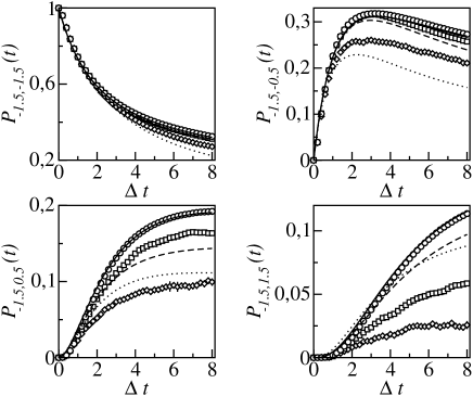
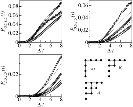
Figure 5: Dissipative dynamics of two correlated charges in a one-dimensional tight binding lattice with $d=5$ sites obtained from PIMC simulations (symbols) and a master equation approach (lines). Shown are the many-body state populations $P_{s,s^{\prime}}$ for the edge states of fig. (4) with either $s=-1.5$ or $s^{\prime}=1.5$. Circles, squares and diamonds denote situations where some sites have been removed from otherwise identical lattices as depicted in a), b), and c), respectively, referring to an increasing connectivity between the allowed sites. Solid (a), dashed (b), and dotted lines (c), respectively, depict the corresponding results from the master equation.

Let us now analyze (iii) in more detail based on (24) with the corresponding transition rates (23). The simplest case is $d=2$ with only three available sites $(-\,{}^{1\!}/_{2},-\,{}^{1\!}/_{2}),(-\,{}^{1\!}/_{2},\,{}^{1\!}/_{2}),(\,{}^{1\!}/_{2},\,{}^{1\!}/_{2})$. Obviously, for this case the triangular lattice coincides with a linear chain with three sites so that if a time local master equation applies for this latter case, it also applies for the two-charge case. For larger $d$, however, the situation changes fundamentally due to a different topology of the two-dimensional lattices which then contain bulk-sites with four adjacent sites (apart from $d=3$ where there is no bulk site, but two edge-sites with three connections). Accordingly, the typical dwell time on a bulk-site is considerably shorter than on a site with two connections, roughly, by a factor of 2. An environment which is able to destroy the phase coherence of the wave function on each site of a linear chain before a jump to an adjacent site takes place, may be too slow to achieve the same on bulk-sites in a 2d-lattice. Hence, entangled many body states can survive on such a long time scale that a description based on a master equation local in time fails. In fact, this can be seen in fig. 5, where PIMC data for $d=4$ are depicted together with the corresponding dynamics of the master equation (24). By successively removing more and more bulk sites from the lattice, the agreement of the PIMC data with the prediction of the master equation, which is rather poor in case of the full lattice, increases, until upon creating a linear chain by removing all bulk states an almost perfect match is regained.

The situation becomes even worse for a larger number of charges $n$ since then the bulk sites of the $n$-dimensional cube attain $2n$ decay channels to adjacent sites, thus reducing the average dwell time by a factor of about $2n$ compared to the one-dimensional case $n=1$. The conclusion is the following: If for a bath characterized by $\omega_{c}$ and $\beta$ a Markovian approximation applies for the dynamics on a 1d-lattice with nearest neighbor coupling $\Delta$, i.e.  $\hbar\beta\omega_{c}<1$ and $\Delta/\omega_{c}\ll 1$, this approximation fails for the multi-charge dynamics, unless $\omega_{c}$ is taken to be very large and temperatures are sufficiently high, roughly, $n\Delta/\omega_{c}\ll 1$ and $n\hbar\beta\omega_{c}<1$. Hence, for most cases only numerical approaches like the PIMC procedure presented here, seem to be applicable.

VII Conclusions

The numerically exact PIMC approach has been pushed further to deal also with spatially continuous systems and correlated many-body dynamics. To better understand the numerical data in certain parameter ranges, to estimate the dissipative quantum dynamics before starting an involved PIMC calculation, and even to develop simplified models capturing the relevant processes, Markovian master equations are of great practical use. To explore their applicability in the above situations, we had to consider generalized tight-binding lattices with either non-equidistant spacing or in higher dimensions. In both cases, additional restrictions must be imposed beyond the constraints known from equidistant one-dimensional TBSs so that for broader ranges of bath parameters no simple description seems to be possible. However, it is surprising that in other domains comprising stronger dissipation and lower temperatures, Markovian master equations can still be found to work quite well, at least qualitatively. Thus, Markovian master equations together with numerically exact PIMC simulations, which often provide the sole mean to check for their validity in a certain scenario, provide a powerful means to study dynamical properties over the full time range. In particular, for the correlated many-body dynamics in presence of dissipation this may open the door to examine the intimate interplay between Coulomb interaction, particle statistics, and phonon baths, e.g. for the charge transport in molecular and mesoscopic structures.

- (1) U. Weiss, Quantum Dissipative Systems, Series in Modern Condensed Matter Physics, Vol. 2 (World Scientific, Singapore, 1998).
- (2) C.W. Gardiner, Quantum Noise (Springer, Berlin, 1991).
- (3) G. Lindblad, Commun. Math. Phys. 48, 119 (1976).
- (4) A.G. Redfield, Adv. Magn. Reson. 1, 1 (1965).
- (5) J. Ankerhold, P. Pechukas, and H. Grabert, Phys. Rev. Lett. 87, 086802 (2001).
- (6) B. Vacchini, Phys. Rev. E 66, 027107 (2002); D. Banerjee, B.C. Bag, S.K. Banik, D.S. Ray, Physica A 318, 6 (2003).
- (7) J. Ankerhold, Europhys. Lett. 61, 301 (2003) ; J. Łucka, R. Rudnicki, and P. Hänggi, Physica A 351, 60 (2005).
- (8) J. Ankerhold, Europhys. Lett. 67, 280 (2004); L. Machura, M. Kostur, P. Hänggi, P. Talkner, and J. Łucka, Phys. Rev. E 70, 031107 (2004); J. Ankerhold, H. Grabert, and P. Pechukas, in: 100 years of Brownian motion, Chaos 15, 026106 (2005).
- (9) R.P. Feynman and F.L. Vernon, Ann. Phys. (N.Y.) 24, 118 (1963).
- (10) A.O. Caldeira and A.J. Leggett, Physica 121A, 587 (1983).
- (11) H. Grabert, P. Schramm, and G.-L. Ingold, Phys. Rep. 168, 115 (1988).
- (12) R. Karrlein and H. Grabert, Phys. Rev. E 55, 153 (1997).
- (13) C.H. Mak and R. Egger, Adv. Chem. Phys. 93,39 (1996).
- (14) D. E. Makarov and N. Makri, Chem. Phys. Lett. 221, 482 (1994).
- (15) W.T. Strunz, L. Diósi, and N. Gisin, Phys. Rev. Lett. 82, 1801 (1999); J.T. Stockburger and H. Grabert, Phys. Rev. Lett. 88, 170407 (2002).
- (16) M.H. Beck, A. Jäckle, G.A. Worth, and H.-D. Meyer, Phys. Rep. 324, 1 (2000).
- (17) A.J. Leggett, S. Chakravarty, A.T. Dorsey, M.P.A. Fisher, A. Garg, and W. Zwerger, Rev. Mod. Phys. 57, 1 (1987).
- (18) A. Schmid, Phys. Rev. Lett. 51, 1506 (1983); M.P.A. Fisher and W. Zwerger, Phys. Rev. B 32, 6190 (1985).
- (19) R. Egger, C.H. Mak, and U. Weiss, Phys. Rev. E 50, R655 (1994).
- (20) R. Egger and C. H. Mak, J. Phys. Chem. 98, 9903 (1994); L. Mühlbacher and R. Egger, J. Chem. Phys. 118, 179 (2003).
- (21) L. Mühlbacher, J. Ankerhold, and C. Escher, J. Chem. Phys. 121, 12696 (2004).
- (22) L. Mühlbacher, J. Ankerhold, J. Chem. Phys. 122, 184715 (2005).
- (23) M. Thorwart, M. Grifoni, and P. Hänggi, Phys. Rev. Lett. 85, 860 (2000); Ann. Phys. (New York) 293, 15 (2001).
- (24) Quantum Monte Carlo Methods in Condensed Matter Physics, M. Suzuki (ed.) (World Scientific, Singapore, 1993), and references therein.
- (25) R. Egger and C. H. Mak, Phys. Rev. B 50, 15210 (1994).
- (26) C. H. Mak, R. Egger, and H. Weber-Gottschick, Phys. Rev. Lett. 81, 4533 (1998).
- (27) J. Ankerhold and H. Lehle, J. Chem. Phys. 120, 1436 (2004).
- (28) J. Jortner and M. Bixon, eds., Adv. Chem. Phys. 106, 107 (1999); A. Nitzan, Ann. Rev. Phys. Chem. 52, 681 (2001).
- (29) E.G. Petrov and P. Hänggi, Phys. Rev. Lett. 86, 2862 (2001); J. Lehmann, G.-L. Ingold, and P. Hänggi, Chem. Phys. 281, 199 (2002).