Perturbative continued-fraction method for weakly interacting Brownian spins and dipoles

J. L. Garcรญa-Palacios

The continued-fraction (CF) method was developed systematically by Risken and co-workers to solve problems of arbitrary fluctuations in nonlinear systems[1]. However, this efficient technique is limited to problems with a few variables,[2] which in practice means systems of noninteracting entities (particles, spins, etc.) In this communication, we illustrate how to extend the CF method to weakly coupled systems with the problem of relaxation in classical spins.

The Fokkerโ€“Planck equation governing the Tโ‰ 0๐‘‡0T\neq 0 dynamics of a classical spin sโ†’โ†’๐‘ \vec{s} is given by[3]


2โ€‹ฯ„Dโ€‹โˆ‚Wโˆ‚t=โˆ’โˆ‚โˆ‚sโ†’โ‹…{1ฮปโ€‹sโ†’โˆงBโ†’โˆ’sโ†’โˆง[sโ†’โˆง(Bโ†’โˆ’โˆ‚โˆ‚sโ†’)]}โ€‹W,2subscript๐œD๐‘Š๐‘กโ‹…โ†’๐‘ 1๐œ†โ†’๐‘ โ†’๐ตโ†’๐‘ delimited-[]โ†’๐‘ โ†’๐ตโ†’๐‘ ๐‘Š\displaystyle 2\tau_{{\rm D}}\frac{\partial W}{\partial t}=-\frac{\partial{}}{\partial\vec{s}}\cdot\left\{\frac{1}{\lambda}\vec{s}\wedge\vec{B}-\vec{s}\wedge\left[\vec{s}\wedge\left(\vec{B}-\frac{\partial{}}{\partial\vec{s}}\right)\right]\right\}W\;,

where $\lambda$ is the dissipation parameter, Bโ†’=โˆ’(โˆ‚โ„‹/โˆ‚sโ†’)โ†’๐ตโ„‹โ†’๐‘ \vec{B}=-(\partial{\cal H}/\partial\vec{s}) the effective field, and $\tau_{{\rm D}}\propto T^{-1}$ the free diffusion time. If we write this equation as $\partial W/\partial t={\cal L}_{\rm FP}W$, the dynamical equation for any average $\left\langle f\right\rangle$ is given in terms of the adjoint Fokkerโ€“Planck operator by dโ€‹โŸจfโŸฉ/dโ€‹t=โŸจโ„’FPโ€ โ€‹fโŸฉddelimited-โŸจโŸฉ๐‘“d๐‘กdelimited-โŸจโŸฉsuperscriptsubscriptโ„’FPโ€ ๐‘“{\rm d}\left\langle f\right\rangle/{\rm d}t=\langle{\cal L}_{\rm FP}^{\dagger}f\rangle.

However, the underlying Landauโ€“Lifshitz damping term โˆ’ฮปโ€‹sโ†’โˆง(sโ†’โˆงBโ†’)๐œ†โ†’๐‘ โ†’๐‘ โ†’๐ต-\lambda\vec{s}\wedge\big{(}\vec{s}\wedge\vec{B}\big{)} is nonlinear in sโ†’โ†’๐‘ \vec{s} and couples the equations for the moments. To handle the infinite systems of coupled equations it is convenient to introduce the spherical harmonics Xlm=eiโ€‹mโ€‹ฯ†โ€‹Plmโ€‹(sz)superscriptsubscript๐‘‹๐‘™๐‘šsuperscript๐‘’i๐‘š๐œ‘superscriptsubscript๐‘ƒ๐‘™๐‘šsubscript๐‘ ๐‘งX_{l}^{m}=e^{{\rm i}m\varphi}P_{l}^{m}(s_{z}), and take advantage of their recurrence relations. Writing โ„’FPโ€ superscriptsubscriptโ„’FPโ€ {\cal L}_{\rm FP}^{\dagger} in terms of the rotation operator ๐’ฅโ†’=โˆ’iโ€‹sโ†’โˆง(โˆ‚/โˆ‚sโ†’)โ†’๐’ฅiโ†’๐‘ โ†’๐‘ \vec{{\cal J}}=-{\rm i}\,\vec{s}\wedge(\partial{}/\partial\vec{s})

โ„’FPโ€ =โˆ’iฮปโ€‹Bโ†’โ‹…[๐’ฅโ†’+ฮปโ€‹(sโ†’โˆง๐’ฅโ†’)]โˆ’๐’ฅโ†’2,superscriptsubscriptโ„’FPโ€ โ‹…i๐œ†โ†’๐ตdelimited-[]โ†’๐’ฅ๐œ†โ†’๐‘ โ†’๐’ฅsuperscriptโ†’๐’ฅ2{\cal L}_{\rm FP}^{\dagger}=-{\textstyle{{\rm i}\over\lambda}}\vec{B}\cdot\big{[}\vec{{\cal J}}+\lambda\big{(}\vec{s}\wedge\vec{{\cal J}}\big{)}\big{]}-\vec{{\cal J}}^{2}\;, (1)

we get the equations for the $X_{l}^{m}$ in the form of a recurrence relation that can be solved by CF methods.

When the spins interact, the structure of โ„’FPโ€ superscriptsubscriptโ„’FPโ€ {\cal L}_{\rm FP}^{\dagger} is the same with the field created by the other spins $\vec{b}_{\rm d}$ included in $\vec{B}$. This allows to separate the free evolution and interaction terms, โ„’FPโ€ =โ„’FP,0โ€ +bโ†’dโ‹…๐’ฅโ†’LLsuperscriptsubscriptโ„’FPโ€ superscriptsubscriptโ„’FP0โ€ โ‹…subscriptโ†’๐‘dsubscriptโ†’๐’ฅLL{\cal L}_{\rm FP}^{\dagger}={\cal L}_{{\rm FP},0}^{\dagger}+\vec{b}_{\rm d}\cdot\vec{{\cal J}}_{\rm LL}, where $\vec{{\cal J}}_{\rm LL}$ is the operator multiplying $\vec{B}$ in Eq.ย (1). For weak coupling, we can expand the averages in the coupling parameter $\left\langle f\right\rangle=\left\langle f\right\rangle_{0}+\left\langle f\right\rangle_{1}+\cdots$, getting a hierarchy of equations

$\displaystyle{\rm d}\left\langle f\right\rangle_{0}/{\rm d}t$ $\displaystyle=$ โŸจโ„’FP,0โ€ โ€‹fโŸฉ0subscriptdelimited-โŸจโŸฉsuperscriptsubscriptโ„’FP0โ€ ๐‘“0\displaystyle\big{\langle}{\cal L}_{{\rm FP},0}^{\dagger}\,f\big{\rangle}_{0}
$\displaystyle{\rm d}\left\langle f\right\rangle_{1}/{\rm d}t$ $\displaystyle=$ โŸจโ„’FP,0โ€ โ€‹fโŸฉ1+โŸจbโ†’dโ‹…๐’ฅโ†’LLโ€‹fโŸฉ0subscriptdelimited-โŸจโŸฉsuperscriptsubscriptโ„’FP0โ€ ๐‘“1subscriptdelimited-โŸจโŸฉโ‹…subscriptโ†’๐‘dsubscriptโ†’๐’ฅLL๐‘“0\displaystyle\big{\langle}{\cal L}_{{\rm FP},0}^{\dagger}\,f\big{\rangle}_{1}+\big{\langle}\vec{b}_{\rm d}\cdot\vec{{\cal J}}_{\rm LL}\,f\big{\rangle}_{0}
$\displaystyle{\rm d}\left\langle f\right\rangle_{2}/{\rm d}t$ $\displaystyle=$ โŸจโ„’FP,0โ€ โ€‹fโŸฉ2+โŸจbโ†’dโ‹…๐’ฅโ†’LLโ€‹fโŸฉ1subscriptdelimited-โŸจโŸฉsuperscriptsubscriptโ„’FP0โ€ ๐‘“2subscriptdelimited-โŸจโŸฉโ‹…subscriptโ†’๐‘dsubscriptโ†’๐’ฅLL๐‘“1\displaystyle\big{\langle}{\cal L}_{{\rm FP},0}^{\dagger}\,f\big{\rangle}_{2}+\big{\langle}\vec{b}_{\rm d}\cdot\vec{{\cal J}}_{\rm LL}\,f\big{\rangle}_{1}
$\displaystyle\vdots$

To illustrate our procedure, let us denote by $X_{\ell}^{m}$ and $Y_{p}^{q}$ the spherical harmonics of two of the spins, and consider the equation for $X_{\ell}^{m}$ (i.e., $f=X_{\ell}^{m}$ above). Since the field created by the second spin depends on $Y_{p}^{q}$, one needs $\left\langle X_{\ell}^{m}\,Y_{p}^{q}\right\rangle_{i}$, $i=0,1$, which could be obtained writing the above equations also for $f=X_{\ell}^{m}\,Y_{p}^{q}$. This leads to another complication, since $\vec{b}_{\rm d}\cdot\vec{{\cal J}}_{\rm LL}\,f$ then involves products of three spherical harmonics. However, $Y_{1}^{\mu}Y_{p}^{q}$ can be expanded as a linear combination of the $Y_{p}^{q}$โ€™s, restoring a structure solvable by CF methods.

These manipulations result in a complicated algorithm, so it is convenient to check it out against some solvable case. Fortunately, for freely rotating spins the problem reduces to that of electric dipoles, where the perturbative calculation can be done analytically, yielding[4]


$\displaystyle\frac{\alpha(\omega)}{\alpha_{0}(\omega)}=1\!-\!\frac{\alpha^{2}\varrho^{2}}{1\!+\!{\rm i}\omega\tau_{{\rm D}}}\left\{{\cal R}\left[1\!+\!\frac{{\rm i}\omega\tau_{{\rm D}}}{2(4\!+\!{\rm i}\omega\tau_{{\rm D}})}\right]{}-\frac{{\cal S}}{1\!+\!{\rm i}\omega\tau_{{\rm D}}}\right\}$

where ฮฑ0โ€‹(ฯ‰)subscript๐›ผ0๐œ”\alpha_{0}(\omega) and ฮฑ๐›ผ\alpha (โˆTโˆ’1proportional-toabsentsuperscript๐‘‡1\propto T^{-1}) are the dynamic and static polarisabilities of noninteracting dipoles, ฯฑitalic-ฯฑ\varrho is the dipole density, and โ„›โ„›{\cal R} and ๐’ฎ๐’ฎ{\cal S} are certain โ€œlattice sumsโ€ of the interaction tensor. 
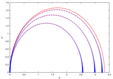
Figure 1 shows that our perturbative CF approach gives accurately the analytical results.

Refer to caption
FIG.โ€„1.: Coleโ€“Cole plots of the dielectric polarisability (imaginary vs. real part) for various couplings $\varrho$. Lines: Zwanzig formula; crosses: perturbative CF results.

Therefore, this approach extends the applicability of the efficient CF techniques to (weakly) interacting systems, and allows one to handle problems involving driven systems, evolving in nonlinear potentials, coupled, and subjected to dissipation and fluctuations

The author acknowledges financial support from DGES (PB98-1592) and F. Falo for useful discussions.

REFERENCES

  • โˆ— wzar.unizar.es/acad/fac/cie/cond-mat/T/theory.html
  • 1 H. Risken, The Fokkerโ€“Planck Equation (Springer, 1989).
  • 2 P. Hรคnggi et al., Rev. Mod. Phys., 62, 251 (1990)
  • 3 W.ย F. Brown, Jr., Phys. Rev. 130, 1677 (1963).
  • 4 R. Zwanzig, J. Chem. Phys. 38, 2766 (1963)