Domain Growth, Budding, and Fission in Phase Separating Self-Assembled Fluid Bilayers

Abstract

A systematic investigation of the phase separation dynamics in self-assembled multi-component bilayer fluid vesicles and open membranes is presented. We use large-scale dissipative particle dynamics to explicitly account for solvent, thereby allowing for numerical investigation of the effects of hydrodynamics and area-to-volume constraints. In the case of asymmetric lipid composition, we observed regimes corresponding to coalescence of flat patches, budding, vesiculation and coalescence of caps. The area-to-volume constraint and hydrodynamics have a strong influence on these regimes and the crossovers between them. In the case of symmetric mixtures, irrespective of the area-to-volume ratio, we observed a growth regime with an exponent of $1/2$. The same exponent is also found in the case of open membranes with symmetric composition.

I INTRODUCTION

Biomembranes are fascinating self-assembled quasi-two-dimensional complex fluids composed essentially of phospholipids and cholesterol. The primary roles of biomembranes are the separation between the inner and outer environments of the cell or inner organelles, and the support of an amazing specialized protein-based machinery which is crucial for a variety of physiological functions, transmembrane transport and structural integrity of the cell alberts94 . Many recent experiments demonstrated that biomembranes of eukariotic cells are laterally organized into small nanoscopic domains, called rafts, which are rich in sphingomyelin and cholesterol. The higher content of cholesterol in rafts is due to the fact that the acyl chains in sphingomyelin are mainly saturated, thereby promoting their interaction with cholesterol. Although, it is largely believed that this inplane organization is essential for a variety of physiological functions such as signaling, recruitment of specific proteins and endocytosis gousset02 , elucidation of the fundamental issues including the mechanisms leading to the formation of lipid rafts, their stability, and finite size remain elusive. Clearly, raft formation in biomembranes is complicated by the presence of many non-equilibrium mechanisms. In view of this, it is important to understand the equilibrium phase behavior and the kinetics of fluid multicomponent lipid membranes before attempts are made to find the effects of more complex mechanisms that may be involved in the formation and stability of lipid rafts.

The dynamics of in-plane demixing in multicomponent lipid membranes is richer than their counterparts in Euclidean three- or two-dimensional systems. This is largely due to (i) the strong coupling between the lipid composition and the membrane conformation, (ii) the difference between the viscosities of the lipid bilayer and that of the embedding fluid, and (iii) the area-to-volume constraint, maintained by a gradient in osmotic pressure across the membrane. As a result, various growth regimes, may be observed in multicomponent lipid membranes. Phase separation dynamics in multicomponent vesicles following a quench from a single homogeneous phase to the two-phase liquid-liquid coexistence region of the phase diagram has previously been considered by means of a generalized time-dependent Ginzburg-Landau model on a non-Euclidean closed surface taniguchi96 ; voth05 . Limitations imposed by the parameterization of surface deformations did not allow for budding in this study. More recent simulations using a dynamic triangulation Monte Carlo model kumar96 ; kumar98 ; kumar01 , predicted dynamics which are much more complex than that in Euclidean surfaces. In particular, these simulations showed that for symmetric composition of binary mixtures, at intermediate times, the dynamics is characterized by the presence of the familiar labyrinth-like spinodal pattern. At later times, in the presence of curvature composition coupling, these patterns break up leading to isolated islands. At still later times, and in the case of tensionless membranes, these domains reshape into buds connected to the parent membrane by very narrow necks. Further domain growth proceeds via the Brownian diffusion of these buds, and their coalescence. It is important to remark that both the generalized time-dependent Ginzburg-Landau model and the Monte Carlo dynamic triangulation model (1) do not account for the solvent, and are therefore purely dissipative, (2) cannot account for the constraint on the volume enclosed by the vesicle, (3) conserve the topology of the membrane throughout the simulation, and therefore do not account for fission or fusion processes. A model that accounts of these effects is clearly warranted in order to compare with experiments. In order to achieve this we used a model based on the dissipative particle dynamics (DPD) approach  laradji04 .

On the experimental side, recent studies using advanced techniques such as two-photon fluorescence and confocal microscopy, performed on giant unilamellar vesicles (GUVs) composed of dioleoylphosphatidylcholine, sphingomyelin, and cholesterol, showed the existence of lipid domains dietrich01 . More recent experiments on ternary mixtures composed of saturated and unsaturated phosphatidylcholine and cholesterol silvius96 ; keller02 ; baumgart03 saw the existence of liquid-liquid coexistence over a wide range of compositions, an indication that liquid-liquid coexistence in lipid membranes is ubiquitous to a wide variety of ternary lipid mixtures. It must be noted, however, that domains observed in these experiments are comparable to the size of the vesicle (micron-scale), orders of magnitudes larger than rafts in biomembranes. Some of these experiments reported structures with many, more-or-less, curved domains. But these are more akin to caps than fully developed buds. An important question that arises out of these studies is: (1) What role does the solvent hydrodynamics and the volume constraints play during coarsening in multicomponent fluid vesicles? (2) Does the topology change drastically alter the kinetic pathway predicted by simulations that does not allow for topology changes?

In this paper, we present results from extensive numerical simulations of self-assembled lipid vesicles and open membranes using the dissipative particle dynamics approach. We specifically investigated the phase separation dynamics in lipid membranes following a quench from the one phase region to the fluid-fluid coexistence region of the phase diagram. The lipid membrane is composed of self-assembled lipid particles in an explicit solvent, thus accounting for hydrodynamic effects. Furthermore, the parameters of the model are such that the membrane is impermeable to the solvent, thus allowing us to investigate the effect of area-to-volume ratio on the dynamics. We specifically investigated the effects of (1) area-to-volume ratio, (2) line tension, and (3) lipids composition on the dynamics. We find that the path,through which dynamics proceeds, depends on the area-to-volume ratio and composition. In off-critical quenches, in particular, the dynamics proceeds via the coalescence of small flat patches at intermediate times, followed by their budding and vesiculation. At late times, domain growth proceeds via coalescence of caps remaining on the vesicle. Crossovers between these regimes are strongly affected by the area-to-volume ratio and line tension. In the case of critical quenches, domain growth proceeds via dynamics similar to that in Euclidian two-dimensional fluids. That is, in this case the effect on the embedding fluid on the coarsening process seems to be not very obvious. We check this by also by simulating critical quenches in open membranes with different projected areas.

This article is organized as follows: in Sec. II, the model and simulation technique are presented. In Sec. III, results of our simulations are presented. Finally, we summarize and conclude in Sec. IV.

II MODEL AND METHOD

In this work, the dynamics of phase de-mixing of a two-component lipid mixture in an explicit solvent is investigated using dissipative particle dynamics (DPD) approach. DPD was first introduced by Hoogerbrugge and Koelman more than a decade ago hoogerbrugge92 , and was cast in its present form about five years later espagnol95 ; espagnol97 . DPD is reminiscent of molecular dynamics, but is more appropriate for the investigation of generic properties of macromolecular systems. The use of soft repulsive interactions in DPD, allows for larger integration time increments than in a typical molecular dynamics simulation using Lennard-Jones interactions. Thus time and length scales much larger than those in atomistic molecular dynamics simulations can be probed by the DPD approach. Furthermore, DPD uses pairwise random and dissipative forces between neighboring particles, which are interrelated through the fluctuation-dissipation theorem. The pairwise nature of these forces ensures local conservation of momentum, a necessary condition for correct long-range hydrodynamics pagonabarraga98 .

The system is composed of simple solvent particles (denoted as $w$), and two types of complex lipid particles (A and B). A lipid particle is modeled as a flexible amphiphilic chain with one hydrophilic particle, mimicking a lipid head group, and three hydrophobic particles, mimicking the lipid acyl-group. More complicated lipid structures and artifacts due to the choice of simulation parameters have been investigated by other groups ask05 ; shillcock02 ; ilya05 . These details are not expected to affect the qualitative nature of the results reported here.

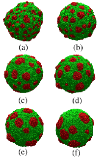
Figure 1: Snapshots of a phase separating vesicle with low excess area, and $\phi_{B}=0.5$ at (a) $t=100\,\tau$, (b) $500\,\tau$, (c) $1000\,\tau$, (d) $2000\,\tau$, (e) $3000\,\tau$, and (f) $4000\,\tau$.

The heads of the A and B lipids are denoted by $h_{A}$ and $h_{B}$, and their respective tails are denoted by $t_{A}$ and $t_{B}$. For simplicity, we focus in this study on the case where the interactions are symmetric under the exchange between $A$ and $B$ lipids. Thus this model does not contain any explicit coupling between curvature and composition. The time evolution of the position and velocity of each dpd particle $i$, denoted by $({\bf r}_{i},{\bf v}_{i})$, are governed by Hamilton’s equations of motion. The three pairwise forces are given by

$${\bf F}^{(C)}_{ij} = a_{ij}\omega(r_{ij}){\bf n}_{ij},$$ (1)

$${\bf F}^{(D)}_{ij} = \gamma_{ij}\omega^{2}(r_{ij})(\hat{\bf r}_{ij}\cdot{\bf v}_{ij}){\bf n}_{ij},$$ (2)

$${\bf F}^{(R)}_{ij} = \sigma_{ij}(\Delta t)^{1/2}\omega(r_{ij})\theta_{ij}{\bf n}_{ij},$$ (3)

where $r_{ij}={\bf r}_{j}-{\bf r}_{i}$, ${{\bf n}}_{ij}={{\bf r}_{ij}}/{r_{ij}}$, and ${\bf v}_{ij}={\bf v}_{j}-{\bf v}_{i}$. $\theta_{ij}$ is a symmetric random variable satisfying

$$\langle\theta_{ij}(t)\rangle = 0,$$ (4)

$$\langle\theta_{ij}(t)\theta_{kl}(t^{\prime})\rangle = (\delta_{ik}\delta_{jl}+\delta_{il}\delta_{jk})\delta(t-t^{\prime}).$$ (5)

with $i\neq j$ and $k\neq l$. In Eq.(3), $\Delta t$ is the iteration time step. The weight factor is chosen as

$$\omega(r)=\left\{\begin{array}[]{ll}1-r/r_{c}&\mbox{ for $r\leq r_{c}$,}\\ 0&\mbox{ for $r>r_{c}$}\end{array}\right.$$ (6)

where $r_{c}$ is the interactions cutoff radius. The choice of $\omega$ in Eq. (6) ensures that the interactions are all soft and repulsive. The equations of motion of particle $i$ are given by

$$d{\bf r}_{i}(t) = {\bf v}_{i}(t)dt,$$ (7)

$$d{\bf v}_{i}(t) = \frac{1}{m}\biggl{(}\sum_{j}{\bf F}^{(C)}_{ij}dt+\sum_{j}{\bf F}^{(D)}_{ij}dt$$ (8)

$$+\sum_{j}{\bf F}_{ij}^{(R)}(dt)^{1/2}\biggl{)},$$

where $m$ is the mass of a single DPD particle. Here, for simplicity, masses of all types of dpd particles are supposed to be equal. Assuming that the system is in a heat bath at a temperature $T$, the parameters $\gamma_{ij}$ and $\sigma_{ij}$ in Eqs. (2 and 3) are related to each other by the fluctuation-dissipation theorem,

$$\gamma_{ij}=\sigma_{ij}^{2}/2k_{\rm B}T.$$ (9)

The parameters, $a_{ij}$, of the conservative forces are specifically chosen as

$$a_{ij}=\frac{\epsilon}{r_{c}}\left(\begin{array}[]{cccccc}&h_{A}&t_{A}&w&h_{B}&t_{B}\\ h_{A}&25&200&25&a_{AB}&200\\ t_{A}&200&25&200&200&a_{AB}\\ w&25&200&25&25&200\\ h_{B}&a_{AB}&200&25&25&200\\ t_{B}&200&a_{AB}&200&200&25\end{array}\right),$$ (10)

where $\epsilon$ and the cutoff radius, $r_{c}$, set the energy and length scales, respectively. The effect of line tension is studied by varying the parameter $a_{AB}$. The integrity of a lipid particle is ensured via an additional simple harmonic interaction, between consecutive particles, whose force is given by

$${\bf F}_{i,i+1}^{(S)}=-C\left(1-r_{i,i+1}/b\right){{\bf n}}_{i,i+1},$$ (11)

where we set, for the spring constant and the preferred bond length, values $C=100\epsilon$ and $b=0.45r_{c}$, respectively.

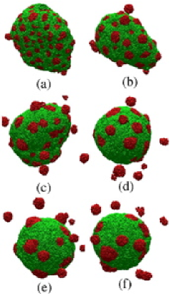
Figure 2: Snapshots of a phase separating vesicle in case-II. The time sequence of the snapshots is the same as in Fig. 1.

In our simulations, we used $\sigma=3.0\left(\epsilon^{3}m/r_{c}^{2}\right)^{1/4}$. Most of the simulations were performed at $k_{B}T=\epsilon$, and a fluid density $\rho=3.0r_{c}^{-3}$. The iteration time was chosen to be $\Delta t=0.05\tau$ footnote1 , with the time scale $\tau=(mr_{c}^{2}/\epsilon)^{1/2}$. The equations of motion are integrated using velocity-Verlet algorithm gerhard . The total number of lipid particles used was $16\ 000$, and both cases of closed vesicles and open membranes were simulated. In the case of a closed vesicle, the box size is $(80\times 80\times 80)r_{c}^{3}$ corresponding to a total number of $1\ 536\ 000$ dpd-particle. In the case of open membranes, we consider box sizes of $L_{x}=L_{y}>L_{z}$, with $L_{z}=40r_{c}$, such that the fluid density is equal to that in the case of closed vesicles. Open membranes with different tensions are simulated by varying $L_{x}$, such that the number of lipid particles and fluid density are kept constant. Note that $L_{z}=40r_{c}$ is still much larger than the thickness of the bilayer. Periodic boundary conditions are applied in all directions for both cases of closed and open membranes.

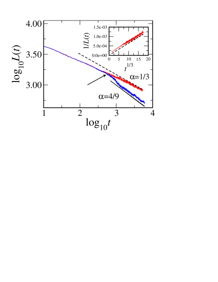
Figure 3: Net interface length as a function of time in case-I (blue curve) and case II (red curve). The green curve corresponds to case II with low line tension (see text for details of corresponding interactions). The dashed lines and the dot-dashed line have slopes of $0.3$ and $4/9$, respectively. In the inset, the number of vesiculated domains is shown as a function of time for case-II with high line tension (corresponding to the red curve). The arrows point to the time regime during which budding and vesiculation occur in case II with high line tension.

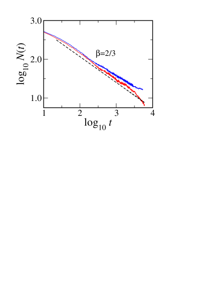
Figure 4: Number of clusters on the vesicle as a function of time. Curve colors correspond to those in Fig. 3. The slope of the dashed line is 2/3. Note that in the case of high excess area, clusters that have vesiculated are excluded.

Previous simulations based on DPD models have shown that open bilayers and closed vesicles can be self-assembled shillcock02 ; yamamoto02 ; yamamoto03 . These studies, however, were performed on smaller systems than those in the present study. In order to save computer time, we prepare our vesicles starting from an almost closed configuration, composed from a single type of lipid. This approach allows for the equilibration of the lipid surface coverage in both leaflets through the diffusion of the lipids via the rim of the open vesicle. We find that the vesicle typically closes within about $50\ 000$ DPD time steps. Once the vesicle is closed, we also found that within our parameters, the number of solvent particles inside the vesicle and the numbers of lipid particles in the inner and outer leaflets remain constant throughout the simulation. A vesicle composed of $16\ 000$ lipid chains, prepared as indicated above, is found to be nearly spherical and contain about $138\ 500$ solvent particles inside it. Vesicles with excess area (high area-to-volume ratio) are then prepared by transferring solvent particles from the core of the vesicles, prepared as indicated above, to the outer region, such that the fluid density is kept constant. An open membrane is prepared by placing a bilayer parallel to the $xy$-plane at $z=L_{z}/2$. The membrane is let to equilibrate until fluctuations of its height attain saturation. After equilibration of the closed vesicle or the open membrane, the phase separation process is triggered through an instantaneous change of a fraction of the A-lipids to B-lipids such that their composition is equal to $\phi_{B}$. This mimics a quench from a homogeneous state to the two-phase region.

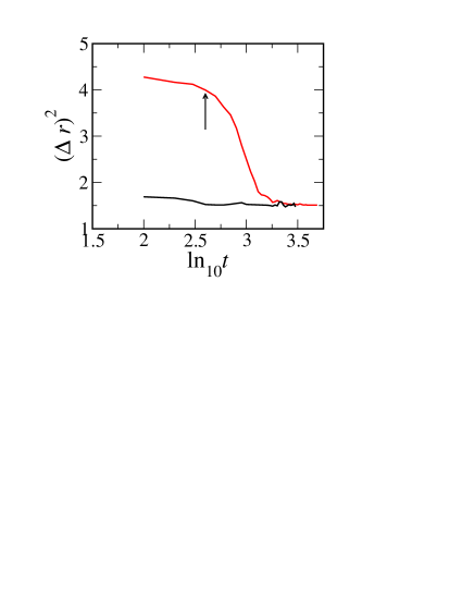
Figure 5: Mean square of the distance of the A-lipids from the center of mass. The top and bottom curves correspond to $\nu=0.17$ and $0.14$, respectively.

We have performed systematic simulations in which following parameters were varied:
(i) The strength of the repulsive interaction between A and B lipids, $a_{AB}$, in order to infer the effect of line tension, $\lambda$, between A and B domains. This parameter was varied for both open and closed membranes.
(ii) The compositions of the two lipids, $\phi_{A}$ and $\phi_{B}=1-\phi_{A}$. We considered the cases of $\phi_{A}=0.5$ and $0.3$. This parameter was varied for both closed and open membranes.
(iii) The area-to-volume ratio, $\nu$, in the case of closed vesicles, defined here as $\nu=\left(N_{head}+N_{tail}\right)/{N_{w}}$, where $N_{head}$, $N_{tail}$ are the total numbers of head and tail dpd particles, respectively, and $N_{w}$ is the total number of solvent particles inside the vesicle. In the case of open membranes, the projected area, effectively plays the role of area-to-volume ratio in closed vesicle.

In the presentation and discussion of our results, we use the following labels to indicate the parameters used for different simulated systems

system	$\nu$	$a_{AB}\ \ \$	$\phi_{B}$
${\cal A}^{(100)}_{1}$	$0.462$	$100$	$0.3$
${\cal A}^{(100)}_{2}$	$0.567$	$100$	$0.3$
${\cal A}^{(86)}_{2}$	$0.567$	$86$	$0.3$
${\cal A}^{(68)}_{2}$	$0.567$	$68$	$0.3$
${\cal A}^{(50)}_{2}$	$0.567$	$50$	$0.3$
${\cal C}^{(100)}_{1}$	$0.462$	$100$	$0.5$
${\cal C}^{(100)}_{2}$	$0.567$	$50$	$0.5$
${\cal C}^{(50)}_{2}$	$0.567$	$50$	$0.5$

The interaction parameters of the present model are selected such that the membrane is impermeable to solvent particles. This implies that the number of solvent particles inside closed vesicles is constant, thereby allowing us to effectively investigate the effect of area-to-volume ratio. In experiments, this parameter is controlled via the osmotic pressure.

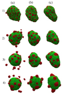
Figure 6: Snapshot sequences for closed vesicles with excess area parameter $\nu=0.17$. (a), (b) and (c) correspond to $a_{AB}=100\epsilon$, $68\epsilon$ and $50\epsilon$, respectively. Snapshots from top to bottom correspond to $t=100\tau$, $1000\tau$, $2000\tau$, and $4000\tau$, respectively.

III RESULTS AND DISCUSSION

For the parameter values mentioned above, our model membrane does not show any flip-flop motion of the lipids, i.e. throughout the simulation time the number of lipids in the upper and lower membrane are the same. We also find that the coupling between the compositions of the two leaflets is found to be very strong. This is not surprising, considering the fact that we have chosen $a_{t_{A}t_{B}}>a_{t_{A}t_{A}}=a_{t_{B}t_{B}}$.

III.1 Case of closed vesicles with $\phi_{B}=0.3$

In Fig. 1, snapshots of closed vesicles configurations in the case of $\phi_{B}=0.3$ and with small area-to-volume ratio, corresponding to system ${\cal A}_{1}^{(100)}$ are shown. This figure shows that the phase separation process after a quench to the two-phase region proceeds in a manner similar to that in Euclidian systems, i.e., through the formation of small domains, and their coalescence in time. During the early stages of the dynamics, domains have average curvatures that are equal to the surrounding majority component, an indication that during the early stages of the phase separation process, the curvature is decoupled from the composition. This is due to the fact that the compositions in the two leaflets are equal, and the A- and em B-lipids have identical architectures, leading to a decoupling between curvature and composition. As time evolves, the interface tension starts to assert and the domains curve very slightly from the majority component, while the vesicle becomes more spherical, an implication that an increase in tension has occurred. In Fig. 2, snapshots corresponding to $\phi_{B}=0.3$, but with a high excess area parameter , ${\cal A}_{2}^{(100)}$, are shown. The high excess area is obtained by removing $25610$ solvent particles from the core of the vesicle and putting them in the outer region, such that the fluid density is maintained. Notice, here again, that during the early stages, domains have same curvature as the majority component, implying the decoupling between curvature and composition during these stages. At about $400\tau$, B-domains start to curve away from the average vesicle’s curvature.

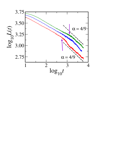
Figure 7: Net interface length versus time for the case of closed vesicles with excess area parameter, $\nu=0.17$, for different values of line tension. Curves from top to bottom correspond to $a_{AB}=50\epsilon$, $68\epsilon$ and $100\epsilon$, respectively.

Domain growth is monitored through both the net interface length, $L(t)$, and the average domain size, $R(t)$, as calculated from the cluster size distribution. In order to see how the interfacial length can be used as a measure of domain coarsening, consider a closed vesicle formed of $N(t)$ B-domains at some time $t$, with an average linear size $R$. Furthermore, let us consider the case where the domains are circular. The net interface length is then given by $L(t)=2\pi N(t)R(t)$. Since the net amount of the B-component, is conserved, we also have for the area occupied by the B-component, ${\cal A}_{B}=\pi N(t)R^{2}(t)$. We therefore have

$$L(t)\sim{\cal A}_{B}/R(t),$$ (12)

and the number of B-domains is therefore given by

$$N(t)\sim{\cal A}_{B}/R^{2}(t).$$ (13)

In Fig. 3, $L(t)$ versus time is shown for the case of $\phi_{A}=0.3$ and for low and high area-to-volume parameter. We notice from this figure that, during intermediate times, i.e. $t<400\tau$, the interfacial length is independent of the area-to-volume ratio, and has the form

$$L(t)\sim t^{-\alpha},$$ (14)

with the growth exponent, $\alpha\approx 0.3$. The number of domains as calculated from the cluster size distribution is shown in Fig. 4, which again shows that the number of clusters is independent of the area-to-volume ratio at intermediate times, and that

$$N(t)\sim t^{-\beta},$$ (15)

with $\beta\approx 2\alpha\approx 2/3$, in agreement with Eq. (13).

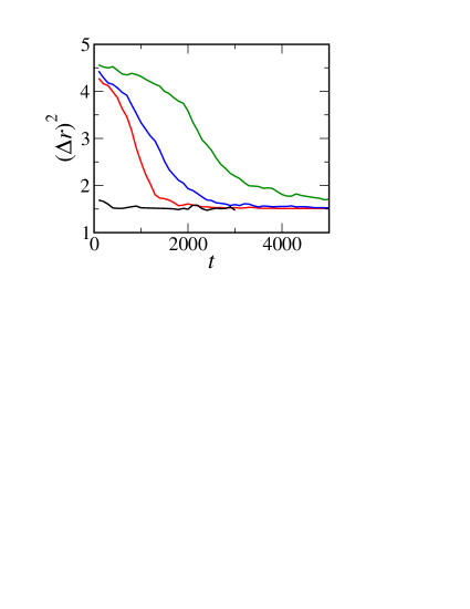
Figure 8: The mean square of the distance of the A-lipid heads from the center of mass, $(\Delta r)^{2}$ versus time. Curves from top to bottom correspond to systems ${\cal A}_{2}^{(50)}$, ${\cal A}_{2}^{(68)}$, ${\cal A}_{2}^{(100)}$, and ${\cal A}_{1}^{(100)}$.

A growth exponent, $\alpha=1/3$, in Euclidian multicomponent systems is usually attributed to the evaporation-condensation mechanism as explained by the classical theory of Lifshitz and Slyozov  lifshitz62 . In a fluid system such as ours, domain growth can also be the result of the motion of the entire domains themselves resulting in collision between domains leading to coalescence.

Two domains coalesce if they travel a distance, $l(t)$ determined by the average area on the membrane occupied by a domain. This is given by

$$l(t)^{2}\sim{\cal A}/N(t).$$ (16)

Moreover, assuming that the domains perform a Brownian walk before their collision, the collision time should obey $l(t)^{2}\sim D_{R}t$. In the case of an isolated two-dimensional fluid, as can be calculated from the Stoke’s formula for the drag on a circular domain due to the surrounding fluid, the diffusion coefficient is independent of the domain size. However, in our case, the drag experienced by the domains results mainly from the three-dimensional embedding fluid, leading to $D_{R}\sim 1/R$. Using this fact, we have the time dependence of domain size as

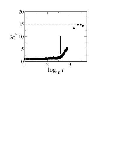
Figure 9: The number of vesiculated buds versus time for system ${\cal A}_{2}^{(100)}$.

$$R(t)\sim t^{1/3},$$ (17)

and the number of clusters

$$N(t)\sim t^{-2/3},$$ (18)

in good agreement with our numerical results.

Irrespective of the initial excess area, the very late times configuration is always that of a tensed vesicle. This can be seen from the mean square of of the positions of the A-lipid heads from the center of mass of the vesicle, $(\Delta r)^{2}$. This is shown in Fig. 5 for the case of $a_{AB}=100\epsilon$, for systems ${\cal A}_{1}^{(100)}$ and ${\cal A}_{2}^{(100)}$. A large $(\Delta r)^{2}$ implies a floppy vesicle with a lot of excess area. Notice that $(\Delta r)^{2}$ decreases rapidly after about $400\tau$, eventually reaching a value equal to that without excess area. The fast decrease in $(\Delta r)^{2}$ is due to the reshaping of the domains into caps, the budding of some of them and their vesiculation. The buds, once formed, are found to vesiculate within a short period of time, of order $10\tau$. We confirm this by performing simulations of a single B-domain occupying $12\%$ of the total area of a vesicle with excess area. The fission mechanism of a bud itself is a very interesting phenomena, and has recently been investigated in detail using DPD simulations yamamoto02 .

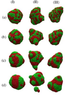
Figure 10: Snapshot sequences of closed vesicles with $\phi_{B}=0.5$. (I), (II) and (III) correspond to systems ${\cal C}_{1}^{(100)}$, ${\cal C}_{2}^{(100)}$ and ${\cal C}_{2}^{(50)}$, respectively. Snapshots from top to bottom correspond to $t=100\tau$, $200\tau$, $400\tau$ and $700\tau$, respectively.

As a result of vesiculation, the parent vesicle looses most of its excess area, leading it to acquire a more spherical shape, as shown in Fig. 2, and implied by Fig. 5. This induced lateral tension prevents the domains from further capping. Further domain coarsening may therefore proceed via the coalescence of these caps.

III.2 Effect of line tension on the phase separation in closed vesicles with $\phi_{B}=0.3$

The effect of line tension on the dynamics of domain growth in closed vesicles with $\phi_{B}=0.3$ is investigated by performing simulations at different values of $a_{AB}=100\epsilon$, $86\epsilon$, $68\epsilon$, and $50\epsilon$ in the presence of large excess area.

In Fig. 6, snapshots for the cases of $a_{AB}=100\epsilon$, $68\epsilon$ and $50\epsilon$ are shown for comparison. These snapshots clearly show that the line tension play an important role on the dynamics. Corresponding interfacial lengths as a function of time are shown in Fig. 7. This figure again shows that budding is delayed as the line tension is increased. We also notice that while in the system with $a_{AB}=100\epsilon$, budding of domains is followed by their vesiculation, in the systems with $a_{AB}=86\epsilon$ and $68\epsilon$, very few buds vesiculate. No vesiculation was observed in the case of low line tension ($a_{AB}=50\epsilon$).

In order to gain further insight into the effect of line tension on domains caping, let us consider a circular domain of B-phase with area $a$, surrounded by a sea of A-phase, on a tensionless membrane. Let $c$ be the absolute value of the mean curvature of this domain which is assumed to be uniform. The free energy of the domain is therefore given by

$${\cal E}_{a}=2{\kappa}ac^{2}+{\lambda}{l},$$ (19)

where $\kappa$ and $\lambda$ are the bending modulus and line tension, respectively, and $l$ is the perimeter of the domains, given by

$${l}=2\pi\left(\frac{a}{\pi}\right)^{1/2}\left(1-\frac{ac^{2}}{4\pi}\right)^{1/2}.$$ (20)

The free energy is then rewritten as

$${\cal E}=8\pi\kappa\left[{\tilde{c}}^{2}+\frac{\lambda}{2\kappa c_{max}^{2}}\left(1-{\tilde{c}}^{2}\right)^{1/2}\right],$$ (21)

where $a=4\pi/c_{max}^{2}$ and ${\tilde{c}}=c/c_{max}$. The free energy in Eq. (21) has a minimum at $c=0$. This minimum is absolute if the area of the domain is smaller than $a_{0}=4\pi(\kappa/\lambda)^{2}$. Otherwise, the free energy is lower for $c>0$. These calculations imply that for a given $\kappa/\lambda$, the onset of domain capping occurs when their average radius exceeds $R_{0}=2\kappa/\lambda$, in qualitative agreement with our simulation results.

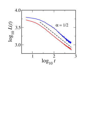
Figure 11: Net interface length versus time for the case of closed vesicles with $\phi_{B}=0.5$. Top and bottom curves correspond to ${\cal C}_{2}^{(100)}$ and ${\cal C}_{2}^{(50)}$, respectively. The slope of the dotted line is 0.5.

In order to verify the arguments above, the bending modulus and line tension for the cases of $a_{AB}=50$ and $100\epsilon$ are extracted numerically. Details of the numerical approach used to derive these quantities are described in Appendices A and B. We obtain a bending modulus $\kappa\approx 8.4\epsilon$, and a line tension $\lambda=7.1\epsilon/r_{c}$ and $5.4\epsilon/r_{c}$. The number of domains at the onset of capping is calculated as

$$N_{c}=\frac{{\cal A}_{v}\phi_{B}}{\pi R_{0}^{2}},$$ (22)

where ${\cal A}_{v}$ is the vesicles area. In the following table, the number of domains at the onset of capping, $N_{c}$, obtained using Eq. (22) and that obtained from the simulations are shown.

	$A^{100}_{2}$	$A^{(50)}_{2}$
$N_{c}$ (from Eq. (22))	91	54
$N_{c}$ (from simulation)	71	38

It is interesting to note that our numerical results are fairly in good agreement with the theoretical values. The discrepancy is reasonable considering the fact that in Eq. (21), only lowest order terms, in curvature, are accounted for. In the simulation, however, a cap is not uniformly curved.

Since domain growth prior to capping is governed by a $t^{1/3}$ law, the onset time of domain capping should be, $t_{cr}\sim(\kappa/\lambda)^{3}$. In the simulation, this time scale is found to be approximately $400\tau$ and $1000\tau$ for systems $A^{(100)}_{2}$ and $A^{(50)}_{2}$, respectively. The ratio between these two times is very close to the ratio of line tensions given by $\left(\lambda_{A^{(50)}_{2}}/\lambda_{A^{(100)}_{2}}\right)^{3}\approx 0.45$.

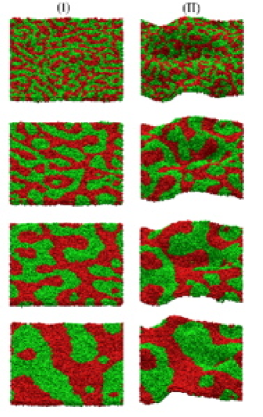
Figure 12: Snapshot sequences for open membranes with $\phi_{B}=0.5$, with $a_{AB}=50$. (I) and (II) correspond to projected areas $L_{x}\times L_{y}=86r_{c}\times 86r_{c}$ and $78r_{c}\times 78r_{c}$, respectively. Snapshots from top to bottom correspond to $t=50\tau$, $200\tau$, $400\tau$ and $800\tau$, respectively.

In Fig. 8, the mean square of the distance of A-lipid heads from the vesicle’s center of mass, $(\Delta r)^{2}$, is plotted for systems, ${\cal A}_{2}^{(100)}$, ${\cal A}_{2}^{(68)}$, ${\cal A}_{2}^{(50)}$, together with the case with small excess area ${\cal A}_{1}^{(100)}$. This figure clearly illustrates that domains capping is shifted towards later times as the line tension is decreased.

III.3 Late time dynamics of closed vesicles with excess area and $\phi_{B}=0.3$

The dynamics in systems ${\cal A}^{(100)}_{1}$ and ${\cal A}^{(100)}_{2}$ departs from each other after about $t=400\tau$, as shown in Fig. 3: The dynamics of domain growth in the case of high excess area speeds up at late times, as compared to the case with low excess area. As shown in Fig. 3, most domains of the minority component in the case with low excess area remain flat with a curvature equal to that of the majority component. Capping, in this case, is suppressed due to the lateral tension induced by volume constraint and low excess area. In contrast, in the case where excess area is high, domains reshape into caps, allowing the interfacial length to decrease rapidly. The presence of excess area allows some of the caps to further reshape into buds as shown in Fig. 2, which then vesiculate, since the line tension is relatively high in this case. Bud vesiculation occurs over a relatively short period of time, as indicated in Fig. 9. We confirm this by performing simulations of a vesicle composed of two coexisting domains and with high excess area. We found that once the bud is formed, it vesiculates within a time period of about $10\tau$.

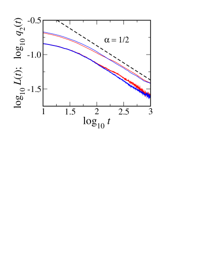
Figure 13: Interfacial length (bold curves) and the square root of the second moment (thin curves) versus time for open membranes with $\phi_{B}=0.5$, with $a_{AB}=50$. Red and blue curves correspond to a projected area $L_{x}\times L_{y}=86r_{c}\times 86r_{c}$ and $78r_{c}\times 78r_{c}$, respectively. The slope of the dotted line is $-1/2$.

The vesiculation of some B-domains results in a marked decrease of excess area leading the vesicle with the remaining B-domains to acquire a much more spherical shape. Once all excess area has been released, domain growth crosses over to a regime characterized by $L(t)\sim t^{-\alpha}$, with $\alpha\approx 0.4$, as shown in Fig. 3. Fig. 4 demonstrates that the number of domains remaining on the vesicle decreases with time as $N_{B}\sim t^{-\beta}$ with a growth exponent $\beta\approx 2/3$.

We believe that the higher growth exponent at late times, $\alpha\approx 0.4$, is the result of coalescence of well formed caps following their Brownian motion. Indeed, as Fig. 1 shows domains of the minority component are more akin to hemispherical caps at late times. Assuming that the curvature of this caps are determined by the competition between the bending energy and the line tension at the interface between A and B lipids, we can write the average interfacial length, $l_{c}$, of a single cap as

$$l_{c}\sim\left(\frac{\kappa a_{c}}{\lambda}\right)^{1/3}.$$ (23)

Domain growth proceeds via the Brownian motion of domains, leading to their coalescence as they collide. Therefore, the mean square of the distance travelled by a single domain,

$$d^{2}\sim Dt,$$ (24)

where $D\sim a_{c}^{-1/2}$, and $d^{2}\sim{\cal A}_{v}/N_{c}$, ${\cal A}_{v}$ being the area of the vesicle. Using as well, the fact that the net area of the $B$-domains is a constant of time, i.e., $N_{c}l_{c}^{3}\sim const$, one then obtains

$$N_{c}\sim\frac{1}{t^{2/3}},$$ (25)

and the net interfacial length, $L_{c}=N_{c}l_{c}$ is then given by

$$L_{c}\sim t^{-4/9},$$ (26)

in excellent agreement with our numerical results.

III.4 Case of closed and open membranes with $\phi_{B}=0.5$

We now focus on the dynamics of phase separation of multicomponent closed vesicles with symmetric volume fractions of the two components. In Fig. 10, snapshots corresponding to the case with high excess area and with high line tension are shown. The corresponding interface length versus time is shown in Fig. 11. This figure shows that the characteristic domain size in the case of $\phi_{B}=0.5$ is much more pronounced than that with asymmetric composition. Furthermore the growth exponent at intermediate times is $\alpha\approx 1/2$, larger than that for the case of $\phi_{B}=0.3$.

We must note that in the case of $\phi_{B}=0.3$, where the lipid domain structure is circular, two measures where used to characterize domain growth. These correspond to the interface length and the average cluster size. In the case of $\phi_{B}=0.5$, only the interface length was so far presented. In order to investigate the robustness of the corresponding growth exponent, $\alpha=1/2$, we also performed simulations of open membranes extending along the $xy$-plane. These simulations allow us to extract another length scale from the composition structure factor, $S(q,t)=\langle|\phi_{\bf q}(t)|^{2}\rangle/L_{x}L_{y}$, as $R(t)=2\pi/q_{2}$, where

$$q_{2}(t)=\left(\frac{\int dqq^{2}S(q,t)}{\int dqS(q,t)}\right)^{1/2}$$ (27)

The effect of tension, and thus the influence of bending modes on phase separation, can also be investigated through varying the projected area, $L_{x}L_{y}$.

In Fig. 12, sequences of snapshots of open membranes with $\phi_{B}=0.5$ and projected areas $L_{x}L_{y}=(80\times 80)r_{c}^{2}$ and $(78\times 78)r_{c}^{2}$ are displayed. Corresponding interface length, $L(t)$, and the square root of the second moment, $q_{2}(t)$, are presented in Fig. 13. It is clear from this figure that both lengths scale as $t^{\alpha}$ with $\alpha\approx 1/2$.

The exact mechanism leading to this exponent is not clear at present. A growth exponent, $\alpha=1$, has been predicted in the case of two component fluids with interconnected structures in three-dimensions and is the result of the instability of the tubular domains against the peristaltic modes siggia79 . Such instability does not exist in pure two-dimensional fluids  sanmiguel85 . On the other hand, several simulations on purely two-dimensional fluids based on molecular dynamics toxvaerd93 , model H lookman95 and lattice gas sunil03 , have seen a growth exponent, $\alpha=1/2$: A theoretical argument for this exponent is however lacking. The lipid bilayer, being a two-dimensional fluid embedded in a three-dimensional solvent, is clearly more complicated than a purely two- or three-dimensional fluid.

IV Summary and Conclusions

In summary, we presented a detailed study of the phase separation dynamics of self-assembled bilayer fluid membranes, with hydrodynamic effects, using dissipative particle dynamics. We considered both open and closed membranes, and investigated the effect of composition, line tension and surface tension. In all cases, hydrodynamics is found to affect the coarsening dynamics at all time scales. In the case of closed vesicles with off-critical quenches, rich dynamics was observed, with crossovers depending strongly on line tension, area-to-volume ratio. The early dynamics in this case, is governed by the coalescence of small flat patches. In the presence of excess area, the later dynamics dynamics is characterized by the coalescence of caps. The crossover between the two regimes depends strongly on line tension, and includes an intermediate vesiculation regime for high enough line tension. In the case of tensed vesicles, no crossover is observed in the dynamics. In the case of critical quenches, the growth dynamics is qualitatively different and no crossovers were observed.

Appendix A: Numerical Extraction of the Bending Modulus

The bending modulus is extracted from the power spectrum of the long-wavelength out-of-plane fluctuations of an open lipid membrane, extending along the $xy$-plane, in a box with periodic boundary conditions along the three directions. The Helfrich Hamiltonian of a membrane, in terms of the principal curvatures, $c_{1}({\bf r})$ and $c_{2}({\bf r})$, is given by

$${\cal H}({c_{1}},{c_{2}})=\int^{\cal A}da\left[\sigma+\frac{\kappa}{2}(c_{1}+c_{2}-2c_{0})^{2}+\overline{\kappa}{c_{1}c_{2}}+\cdots\right]$$ (28)

where $\sigma$, $\kappa$ and $\overline{\kappa}$ are the tension, the bending modulus and the Gaussian bending modulus of the membrane respectively. $c_{0}$ is its spontaneous curvature. In the case of a one-component membrane, and if the lipid lateral densities of the two leaflets are equal, the spontaneous curvature vanishes. Furthermore, if the membrane conserves its topology, the integral of the Gaussian term is independent of the membrane conformation. If we assume that the height of the membrane is represented by a single-valued function $h({\bf x})$, and in the case of small fluctuations, the Hamiltonian can be rewritten in the Monge representation as,

$${\cal H}({h})=\int d{\bf x}^{L^{2}}=\left[\frac{\sigma}{2}(\nabla_{\bf x}h)^{2}+\frac{\kappa}{2}(\nabla_{\bf x}^{2}h)^{2}+\cdots\right].$$ (29)

The structure of the membrane can then be inferred from the structure factor, defined as the Fourier transform of the height-height correlation function,

$$S_{h}({\bf q})=\frac{1}{L^{2}}\langle\mid{\tilde{h}}_{\bf q}\mid^{2}\rangle=\biggl{\langle}\mid\int^{L^{2}}d{\bf x}e^{-i{\bf q}\cdot{\bf x}}h({\bf x})\mid^{2}\biggl{\rangle},$$ (30)

where ${\bf q}=(q_{x},q_{y})$. If the higher order powers of $h$ are omitted in the Hamiltonian, and after the equi-partition theorem is invoked, one finds the the membrane height structure factor is given by

$$S_{h}({\bf q})=\frac{2k_{B}T}{\sigma q^{2}+\kappa q^{4}+{\cal O}(q^{6})}.$$ (31)

The membrane position, $h({\bf x})$, is defined as the location of the median point of the hydrophobic region. In Fig. 14, the structure factor for a one component open membrane in a box of dimensions $L_{x}=L_{y}=86r_{c}$ and $L_{z}=40r_{c}$ is shown. The other parameters are exactly the same as those presented in Sec. II. The bending modulus and the tension on the membrane are obtained from examining the structure factor at small wavevectors. The tension on the membrane is found from the intercept of the $\sigma(q)$ vs. $q^{2}$ curve with the $y$-axis where,

$$\sigma(q)=2k_{B}T/q^{2}S_{h}(q).$$ (32)

The bending modulus is obtained from the slope of $\sigma(q)$, at small $q$’s, as illustrated in Fig. 14. We obtained a value $\kappa\approx 8\epsilon$, when $k_{B}T=\epsilon$. The value of $\kappa$ in our model is reasonably in agreement with the experimental values for lipid bilayers.

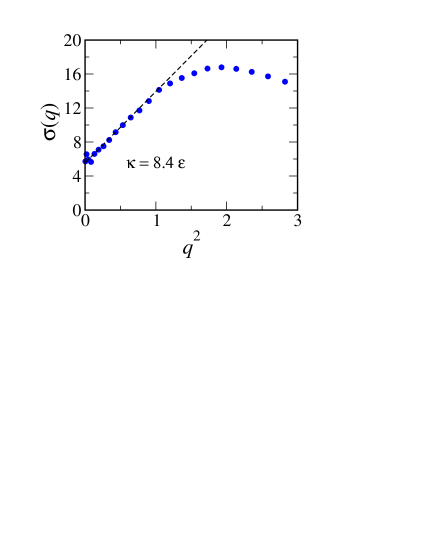
Figure 14: $\sigma(q)=2/q^{2}S_{h}(q)$ versus $q^{2}$ obtained from a simulation of a one-component open membrane with projected area $L_{x}\times L_{y}=86r_{c}\times 86r_{c}$. The slope of the curve at small wavevectors determines the bending modulus, and the intercept with the $y$-axis determines the surface tension of the membrane.

Appendix B: Numerical Extraction of the Line Tension

The in-plane tension of a membrane extending along the $xy$-plane is calculated from the pressure tensor as

$$\sigma=L_{z}\left[P_{zz}-\frac{1}{2}\left(P_{xx}+P_{yy}\right)\right],$$ (33)

where the pressure tensor ${\bf P}_{\alpha\beta}$ is calculated using the Irving-Kirkwood formalism irving50 ,

$${\bf P}=\frac{1}{\Delta V}\sum_{i}\left\langle m_{i}{\bf v}_{i}{\bf v}_{i}+\frac{1}{2}\sum_{i}\sum_{j\neq i}{\bf r}_{ji}{\bf F}^{(C)}_{ji}\right\rangle.$$ (34)

To calculate the line tension, the membrane is prepared such that it consists of A and B coexisting phases, separated by two interfaces which are parallel to the $x$-axis. The tension of the membrane now contains a two-dimensional bulk component plus a one-dimensional contribution due to the interfaces between the A and B components. The line tension is then calculated from the difference between the tension of a membrane with two interfaces between the A and B components and that of a membrane composed with $A$-lipids only,

$$\lambda=\frac{L_{y}}{2}\left(\sigma^{\prime}-\sigma\right).$$ (35)

$\sigma$ and $\sigma^{\prime}$ were calculated on system sizes with dimensions $L_{x}=L_{y}=86r_{c}$ and $L_{z}=40r_{c}$. We found that $\lambda\approx 7.4\epsilon/r_{c}$ and $5.5\epsilon/r_{c}$ for $a_{h_{1}h_{2}}=50\epsilon$ and $100\epsilon$, respectively. If we assume that the lipid bilayer thickness is 4 nm, then our numerically calculated line tensions correspond to $2.3\times 10^{-17}{\rm J}\mu{\rm m}$ and $1.73\times 10^{-17}{\rm J}\mu{\rm m}$, respectively.

Although there are no experimental data for the line tension between coexisting lipid phases, a simple estimation can be given by $\lambda\approx\Delta U/{l}$, where $\Delta U=(U_{AA}-U_{BB})/2-U_{AB}\sim 10k_{B}T$, where $U_{\alpha\beta}$ are the various lipid pair interactions, and $l\approx 0.8$ nm is the lateral length scale associated with a lipid molecule. One then finds $\lambda\sim 10^{-17}{\rm J}\mu{\rm m}$, in agreement with our numerical values sackman95 .

References

- (1) Molecular Biology of the Cell (3rd Ed.) by B. Alberts et al. (Garland Publishing, New York, 1994).
- (2) K. Gousset, W.F. Wolkers, N.M. Tsvetkova, A.E. Oliver, C.L. Field, N. Walker, J. H. Crowe, and F. Tablin, J. Cell. Physiol. bf 190, 117 (2002).
- (3) T. Taniguchi, Phys. Rev. Lett. 76, 4444 (1996).
- (4) G. S.Ayton, J. L. McWhirter, P. McMurtry, and G. A. Voth, Biophys. J. 88, 3855 (2005).
- (5) P.B. Sunil Kumar and M. Rao, Mol. Cryst. Liq. Cryst. 288, 105 (1996).
- (6) P.B. Sunil Kumar and M. Rao, Phys. Rev. Lett. 80, 2489 (1998).
- (7) P.B. Sunil Kumar, G. Gompper, and R. Lipowsky, Phys. Rev. Lett. 86, 3911 (2001).
- (8) M. Laradji and P. B. S. Kumar, Phys. Rev. Lett. 93, 198195 (2004).
- (9) C. Dietrich et al., Biophys. J. 80, 1417 (2001).
- (10) J. Silvius, D. del Giudice, and M. Lafleur, Biochemistry 35, 15198 (1996).
- (11) S.L. Veatch and S.L. Keller, Phys. Rev. Lett. 89, 268101 (2002).
- (12) T. Baumgart, S.T. Hess, and W.W. Webb, Nature (London) 425, 821 (2003).
- (13) P.J. Hoogerbrugge and J.M.V.A. Koelman, Europhys. Lett. 19, 155 (1992).
- (14) P. Espagnol and P. Warren, Europhys. Lett. 30, 191 (1995).
- (15) P. Espagnol, Europhys. Lett. 40, 631 (1997).
- (16) I. Pagonabarraga, M.H.J. Hagen, and D. Frenkel, Europhys. Lett. 42, 377 (1998).
- (17) A.F. Jakobsen, O.G. Mouritsen, and G. Besold, J. Chem. Phys. 122, 204901 (2005).
- (18) J. C. Shillcock and R. Lipowsky, J. chem. Phys. 117, 5048 (2002).
- (19) G. Ilya, R. Lipowsky, and J. C. Shillcock, J. Chem. Phys. 122, 244901 (2005).
- (20) The weak dependence of the surface tension on ask05 does not affect the generic results of the present study.
- (21) G. Besold, I. Vattulainen, M. Karttunen and J. M. Polson, Phys. Rev. E. 62, R7611, (2000).
- (22) S. Yamamoto, Y. Maruyama, and S.-A. Hyodo, J. Chem. Phys. 116, 5842 (2002)
- (23) S. Yamamoto and S.-A. Hyodo, J. Chem. Phys. 118,7893 (2003).
- (24) I. L. Lifshitz and V.V. Slyozov, J. Phys. Chem. Solids 19, 35 (1962).
- (25) E. D. Siggia , Phys. Rev. A 20, 595 (1979).
- (26) M. San Miguel, M. Grant, and J. D. Gunton, Phys. Rev. A 31, 1001 (1985).
- (27) E. Velasco and S. Toxvaerd, Phys. Rev. Lett. 71, 388 (1993).
- (28) Y. Wu, F. J. Alaxander, T. Lookman, and S. Chen, Phys. Rev. Lett. 74, 3852 (1995).
- (29) K. C. Lakshmi and P. B. S. Kumar, Phys. Rev. E. 67, 011507 (2003)
- (30) J.H. Irving and J.G. Kirkwood, J. Chem. Phys. 18, 817 (1950).
- (31) Structure and Dynamics of Membranes, edited by R. Lipowsky and E. Sackman (Elsevier, Amesterdam, 1995).