Coherent transport of cold atoms in angle-tuned optical lattices

Abstract

Optical lattices with a large spacing between the minima of the optical potential can be created using the angle-tuned geometry where the 1-D periodic potential is generated by two propagating laser beams intersecting at an angle different from $\pi$. The present work analyzes the coherent transport for the case of this geometry. We show that the potential depth can be kept constant during the transport by choosing a magic value for the laser wavelength. This value agrees with that of the counterpropagating laser case, and the magic wavelength does not depend of the optical lattice geometry. Moreover, we find that this scheme can be used to implement controlled collision experiments under special geometric conditions. Finally we study the transport of hyperfine-Zeeman states of rubidium 87.

I Introduction

Neutral atoms trapped in an artificial periodic potential formed by laser light, the so called far detuned optical lattice, have been proposed as the individual qubits for quantum information processing. In an optical lattice, neutral atoms can be trapped in the intensity maxima (or minima) of a standing wave light field owing to the optical dipole force. A configuration with one single atom trapped in each site of the optical lattice is realized in the configuration of a Mott-insulator transition associated to the loading of Bose-Einstein condensates (BECs) in optical latticesbloch05 . In order to realize quantum gates with neutral atoms within the ideal environment of the Mott insulator several schemes have been proposed. The common idea is to control the quantum atomic states through the preparation and coherent manipulation of atomic wave-packets by means of application of standard laser cooling and spectroscopic techniques. By using spin dependent, or more precisely state dependent, optical lattice potentials, the control can be applied independently to multiple atomic qubits based on different internal states. A state dependent potential may be created for a one dimensional optical lattice in the so-called lin-$\theta$-lin configuration, where the travelling laser beams creating the optical lattice are linearly polarized with an angle $\theta$ between their polarizations finkelstein92 ; taieb93 ; marksteiner95 . In this configuration the optical potential can be expressed as a superposition of two independent optical lattices, acting on different atomic states. By appropriately choosing the atomic internal states, the atoms will be trapped by one of the two potentials depending on their internal state. By changing the angle $\theta$ between the linear polarizations of the two laser beams producing the optical lattice, the wavepackets corresponding to orthogonal atomic states can be coherently transported relative to each other brennen99 ; jaksch99 ; jaksch05a . Once the atomic qubits are brought together they interact through controlled collisions. In the coherent transport experiment of Mandel et al mandel03 , by a proper control of the angle $\theta$ the wavepacket of an atom initially localized at a single lattice site was split into a superposition of two separate wave packets, and delocalized in a controlled and coherent way over a defined number of lattice sites of the optical potential.
In an optical lattice created by the counterpropagating standing wave configuration, the spacing between neighboring minima of the optical lattice potential is one half the wavelength of the lasers creating the optical lattice. Optical lattices with more widely separated wells can be produced using long wavelength lasers, as CO₂ lasers friebel98 . Alternatively, optical lattices with a larger spacing between the minima/maxima of the optical potential are formed using the angle-tuned geometry. There the periodic potential is created by two laser beams propagating at an angle $\phi$ and the lattice constant is $d=\pi/\left[k\sin(\phi/2)\right]$,with $k=2\pi/\lambda$ the laser wavenumber morsch01 ; hadzibabic04 ; albiez05 ; fallani05 .
The aim of the present work is to analyze the coherent transport associated to the lin-$\theta$-lin polarization configuration for the angle-tuned lattice geometry. We analyze rubidium atoms in a given Zeeman level of a hyperfine state loaded within a 1-D optical-lattice. The 1-D geometry of the Bose gas may be generated by a tight confinement along the orthogonal directions. For instance a two-dimensional array of 1-D Bose gases (tubes) is produced by confining the atoms through a two-dimensional optical lattice generated by independent lasers, as realized in Ref. moritz03 .
Section II defines the geometry of the angle-tuned optical lattice. In Section III we analyze the effective optical potential created by an optical lattice in the angle-tuned configuration. The potential contains a component with a vectorial symmetry described through an effective magnetic field, as derived in deutsch98 . The dependence of the potential depth on the angles defining the lattice geometry is analyzed in Section IV. Section V reexamines the coherent transport for the counterpropagating laser geometry. Section VI extends the coherent transport to the angle-tuned geometry and determines the condition for a constant optical lattice depth during transport. The application to the hyperfine-Zeeman states of rubidium is presented in Sec VII, and in the following Section the minimum time required to realize the coherent transport in the adiabatic limit is briefly discussed.

II Laser geometry

The lasers generating the 1-D lin-$\theta$-lin configuration are composed by two phase-correlated propagating electric fields with frequency $\omega$ and amplitude $E_{0}$. Their wavevectors

$$\begin{split}{\bf k}^{\rm f}_{1}&=k(0,\cos\left(\phi/2\right),\sin\left(\phi/2\right)),\\ {\bf k}^{\rm f}_{2}&=k(0,\cos\left(\phi/2\right),-\sin\left(\phi/2\right))\end{split}$$ (1)

lying on the $(y,z)$ plane create the angle-tuned geometry with angle $\phi$, as shown in Fig. 1. The spatio-temporal dependencies of the electric fields are

$${\bf{\cal E}}^{\rm f}_{j}({\bf x},t)={\bf E}^{\rm f}_{j}({\bf x})e^{-i\omega t}+c.c.=\frac{E_{0}}{2}e^{i\left({{\bf k}^{\rm f}_{j}{\bf x}-\omega t}\right)}{\hat{\bf e}}^{\rm f}_{j}+c.c.\,,$$ (2)

for $j=1,2$, with polarizations ${\bf\hat{e}}^{\rm f}_{j}$ defined in the following. This geometry creates a 1D optical lattice along the $z$-axis. The laser fields confining along the transverse directions are not required for the following analysis and not listed here.

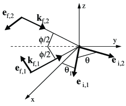
Figure 1: Laser configuration determining the angle tuned geometry. The laser fields propagate within the $(y,z)$ plane with wavevectors ${\bf k}^{\rm f}_{i}$ at an angle $\phi$ between them, and polarizations ${\hat{\bf e}}^{\rm f}_{j}$, with $(j=1,2)$. These wavevectors and polarizations are generated applying the rotations described in the text to two laser fields counterpropagating along the $z$ axis and with polarizations ${\hat{\bf e}}^{\rm i}_{j}$, with $(j=1,2)$ within the $(x,y)$ plane.

The above laser geometry is obtained by applying proper spatial rotations to a 1D optical lattice initially created by two counterpropagating laser fields along the $z$ axis. Let’s introduce the rotation $R_{\rm x}(\alpha)$ of an angle $\alpha$ around the $x$ axis

$$R_{\rm x}(\alpha)=\begin{bmatrix}1&0&0\\ 0&\cos\alpha&-\sin\alpha\\ 0&\sin\alpha&\cos\alpha\end{bmatrix}$$ (3)

and the rotation $R_{\rm z}(\alpha)$ of an angle $\alpha$ around the $z$ axis

$$R_{\rm z}(\alpha)=\begin{bmatrix}\cos\alpha&-\sin\alpha&0\\ \sin\alpha&\cos\alpha&0\\ 0&0&1\end{bmatrix}\,.$$ (4)

In the lin-$\theta$-lin counterpropagating configuration the laser wavevectors are

$${\bf k}^{\rm i}_{1}=k(0,0,1),\quad{\bf k}^{\rm i}_{2}=k(0,0,-1),$$ (5)

and their polarizations, ${\bf\hat{e}}^{\rm i}_{\rm j}$ for $j=(1,2)$, are

$$\begin{split}{\bf\hat{e}}^{\rm i}_{1}&=R_{\rm z}\left(\theta_{1}\right)\begin{bmatrix}1\\ 0\\ 0\end{bmatrix}\,,\\ {\bf\hat{e}}^{\rm i}_{2}&=R_{\rm z}\left(\theta_{1}+\theta\right)\begin{bmatrix}1\\ 0\\ 0\end{bmatrix}.\end{split}$$ (6)

Notice that, in addition to the angle $\theta$ between the two polarization directions, we have introduced the angle $\theta_{1}$ between the polarization vector ${\bf\hat{e}}^{\rm i}_{1}$ and the $x$ axis. The wavevectors ${\bf k}^{\rm f}_{1,2}$, given by Eq. (1), are obtained applying the following rotations:

$${\bf k}^{\rm f}_{1}=R_{\rm x}(\frac{\phi-\pi}{2}){\bf k}^{\rm i}_{1}\,,\quad{\bf k}^{\rm f}_{2}=R_{\rm x}(\frac{\pi-\phi}{2}){\bf k}^{\rm i}_{2}$$ (7)

Such rotations are applied as well to the polarization vectors note1

$$\begin{split}{\bf\hat{e}}^{\rm f}_{1}&=R_{\rm x}(\frac{\phi-\pi}{2}){\bf\hat{e}}^{\rm i}_{1}\\ {\bf\hat{e}}^{\rm f}_{2}&=R_{\rm x}(\frac{\pi-\phi}{2}){\bf\hat{e}}^{\rm i}_{2}\end{split}$$ (8)

The electric fields ${\bf E}^{\rm f}_{1}({\bf x})$, ${\bf E}^{\rm f}_{2}({\bf x})$ are obtained by substituting Eqs. (7) and (8) into Eq. (2), and the total electric field is given by

$${\bf E}_{\rm L}({\bf x})={\bf E}^{\rm f}_{1}({\bf x})+{\bf E}^{\rm f}_{2}({\bf x})=\frac{E_{0}}{\sqrt{2}}{\bf e}_{\rm L}({\bf x})+c.c.,$$ (9)

where ${\bf e}_{\rm L}({\bf x})$ defines the local polarization, not necessarily unit norm.

III optical potential

The optical potential experienced by the atoms is obtained from the analysis of ref. deutsch98 . For alkali atoms, in the limit that the laser detuning is much larger than the hyperfine splittings in both the P_1/2 and P_3/2 excited states, the optical potential has the following form note2 :

$$\hat{U} =U_{J}\hat{I}+{\bf B}_{eff}\hat{\sigma},$$ (10a)

$$U_{J} =V^{0}\left|{\bf e}^{2}_{L}({\bf x})\right|,$$ (10b)

$${\bf B}_{eff} =-iV^{1}\left[{\bf e}^{*}_{L}({\bf x})\times{\bf e}_{L}({\bf x})\right],$$ (10c)

where, in order to simplify the notation, we introduced the following quantities:

$$\begin{split}V^{0}(\omega)&=\frac{E_{0}^{2}}{2}\left(\frac{2\hat{\alpha}_{D2}}{3}+\frac{\hat{\alpha}_{\rm D1}}{3}\right),\\ V^{1}(\omega)&=\frac{E_{0}^{2}}{2}\left(\frac{\hat{\alpha}_{D1}}{3}-\frac{\hat{\alpha}_{\rm D2}}{3}\right).\end{split}$$ (11)

representing the scalar and vector polarizabilities, derived for instance in park01 . The operators $\hat{I},\hat{{\bf\sigma}}$ are the identity and Pauli operators in the electron ground-state manifold. The polarizabilities ${\tilde{\alpha}}_{D_{1}}$ and ${\tilde{\alpha}}_{D_{2}}$ corresponding to the excitations to the P${}_{\frac{1}{2}}$ and P${}_{\frac{3}{2}}$ excited states respectively, depend on the dipole operator reduced matrix element $\langle J^{\prime}\|{\bf d}\|J=\frac{1}{2}\rangle$ with $J^{\prime}=\frac{1}{2},\frac{3}{2}$:

$$\begin{split}{\tilde{\alpha}}_{D_{1}}=\frac{|\langle J^{\prime}=\frac{1}{2}\|{\bf d}\|J=\frac{1}{2}\rangle|^{2}}{\hbar\Delta_{D_{1}}}\,,\\ {\tilde{\alpha}}_{D_{2}}=\frac{|\langle J^{\prime}=\frac{3}{2}\|{\bf d}\|J=\frac{1}{2}\rangle|^{2}}{\hbar\Delta_{D_{2}}}\,.\end{split}$$ (12)

Here $\Delta_{D_{1,2}}$ is the detuning of the laser frequency $\omega$ from the resonance between the states $|F_{max}=2\rangle$ and $|F^{\prime}_{max}=2\rangle$ or $|F^{\prime}_{max}=3\rangle$, for the D₁ or D₂ lines of ⁸⁷Rb respectively.
The substitution of Eqs. (8) for the local polarization in the right sides of Eqs. (10b) and (10c) leads to

$$\begin{split}U_{J}&=V^{0}\left[1+u(\theta_{1},\theta,\phi)\cos(2\pi\frac{z}{d})\right]\,,\\ {\bf e}_{\rm L}^{*}\times{\bf e}_{\rm L}&=i{\bf b}(\theta_{1},\theta,\phi)\sin(2\pi\frac{z}{d})\end{split}$$ (13)

where $d=\pi(k\sin{\frac{\phi}{2}})^{-1}$ is the period of the optical lattice. The $u(\theta_{1},\theta,\phi)$ parameter describes the spatial dependence of the scalar part of the optical lattice

$$u(\theta_{1},\theta,\phi)=\cos(\theta+2\theta_{1})\cos^{2}(\frac{\phi}{2})+\cos(\theta)\sin^{2}(\frac{\phi}{2})\,.$$ (14)

The spatial components of the effective magnetic field are given by

$$\begin{split}b_{\rm x}(\theta_{1},\theta,\phi)&=-\sin(\theta_{1})\sin(\theta_{1}+\theta)\sin(\phi),\\ b_{\rm y}(\theta_{1},\theta,\phi)&=\sin(2\theta_{1}+\theta)\cos(\frac{\phi}{2}),\\ b_{\rm z}(\theta_{1},\theta,\phi)&=-\sin(\theta)\sin(\frac{\phi}{2}),\end{split}$$ (15)

determining also the module $b=|{\bf b}|$. $u$ and $b$ satisfy the following useful relations:

$$u^{2}(\theta_{1},\theta,\phi)+b^{2}(\theta_{1},\theta,\phi)=1,$$ (16)

and

$$u(\theta_{1}=0,\theta,\phi)=\cos(\theta).$$ (17)

The effective magnetic field ${\bf B}_{eff}$ note3 varies spatially with a $d$ period. Its components along the three axes have amplitudes depending on the angles defining the lattice geometry. If the light field is everywhere linearly polarized, $\theta_{1}=\theta=0$, the effective magnetic field vanishes and the light shift is independent of the magnetic atomic sublevel: ${\hat{U}}({\bf x})=U_{J}({\bf x}){\hat{I}}$. For the counterpropagating geometry, i.e. $\phi=\pi$, investigated by brennen99 ; jaksch99 and implemented in mandel03 , the effective magnetic field is oriented along $z$-axis.

IV Hamiltonian Eigenvalues

Making the assumption of neglecting the kinetic energy of the atoms, the effective potential corresponds to the full hamiltonian acting on the atomic states, and the position $z$ can be treated as an external parameter. If we consider the two-dimensional subspace characterized by the electron spin component, i.e., $|S=\frac{1}{2},m_{S}=\frac{1}{2}\rangle$ and $|S=\frac{1}{2},m_{S}=-\frac{1}{2}\rangle$, the eigenvalues of the hamiltonian are

$$\begin{split}\epsilon_{+}&=V^{0}u\cos(2\pi\frac{z}{d})+V^{1}b\sin(2\pi\frac{z}{d}),\\ \epsilon_{-}&=V^{0}u\cos(2\pi\frac{z}{d})-V^{1}b\sin(2\pi\frac{z}{d}),\\ \end{split}$$ (18)

with a constant term $V^{0}$ left out. These quantities represent the optical potential experienced by the atoms. In an equivalent description, $\epsilon_{\pm}$ define the energies of the $|S,m_{S}=\pm\frac{1}{2}\rangle$ atomic states when the electron spin is aligned along the local direction of the magnetic field, i.e., $\hat{\sigma}=\pm{\bf b}/b$. In fact we write

$$\begin{split}\epsilon_{+}&=U_{J}+|{\bf B}_{eff}\ |,\\ \epsilon_{-}&=U_{J}-|{\bf B}_{eff}|.\\ \end{split}$$ (19)

The eigenvalues $\epsilon_{\pm}$ of Eqs (18) can be expressed as

$$\begin{split}\epsilon_{+}(\theta_{1},\theta,\phi,z)&=U_{0}\cos(2\pi\frac{z}{d}+\gamma_{0}),\\ \epsilon_{-}(\theta_{1},\theta,\phi,z)&=U_{0}\cos(2\pi\frac{z}{d}-\gamma_{0}).\ \end{split}$$ (20)

The potential depth $U_{0}(\theta_{1},\theta,\phi)$ and the relative phase $2\gamma_{0}(\theta_{1},\theta,\phi)$ are given by

$$U_{0} =V^{0}\sqrt{\eta^{2}+(1-\eta^{2})u^{2}},$$ (21a)

$$\gamma_{0} =-\arctan\left(\eta\sqrt{\frac{1}{u^{2}}-1}\right),$$ (21b)

where we have introduced

$$\eta(\omega)=\frac{V^{1}(\omega)}{V^{0}(\omega)}.$$ (22)

Eq. (20) demonstrates the spatial periodicity of the potentials experienced by the atomic eigenstates. Ultracold atoms are trapped at the spatial positions corresponding to the minima of the optical lattice potentials. For positive $U_{0}$, the $z_{+}$ and $z_{-}$ minima positions for the $|S=\frac{1}{2},m_{S}=\frac{1}{2}\rangle$ and $|S=\frac{1}{2},m_{S}=-\frac{1}{2}\rangle$ states respectively are given by

$$\begin{split}\frac{z_{+}}{d}&=\frac{1}{2}\left(1-\frac{\gamma_{0}}{\pi}\right)+l\,,\\ \frac{z_{-}}{d}&=\frac{1}{2}\left(1+\frac{\gamma_{0}}{\pi}\right)+l\,,\end{split}$$ (23)

with $l$ an integer. For instance at $\gamma_{0}=\pi/2$, the $|+\rangle$ atoms are localized at $z_{+}=(l+\frac{1}{4})d$ and the $|-\rangle$ atoms at $z_{-}=(l+\frac{3}{4})d$. At $\gamma_{0}=0$ both species are localized at the $(l+\frac{1}{2})d$ positions.

V Counterpropagating geometry

We consider the case $\phi=\pi$ of an optical lattice created by two counterpropagating laser fields. Then the functions $u$ and $b_{j}$ determining the optical lattice potential reduce to

$$\begin{split}&u=\cos(\theta)\\ &b_{x}=b_{y}=0\\ &b_{z}=-\sin(\theta)\end{split}$$ (24)

For this geometry the functions $u$ and $b_{j}$ do not depend on the angle $\theta_{1}$ but only on the relative angle $\theta$. This is a consequence of the symmetry of the system. Since the two beams forming the optical lattice propagate along the direction $z$, the system is invariant under rotations around that axis.
At $\phi=\pi$ the potential depth $U_{0}(\theta)$ and the phase shift $\gamma_{0}(\theta)$ become

$$\begin{split}U_{0}(\theta)&=V^{0}\sqrt{\eta^{2}+(1-\eta^{2})\cos^{2}(\theta)}\\ \gamma_{0}(\theta)&=-\arctan\left(\eta\tan(\theta)\right)\\ \end{split}$$ (25)

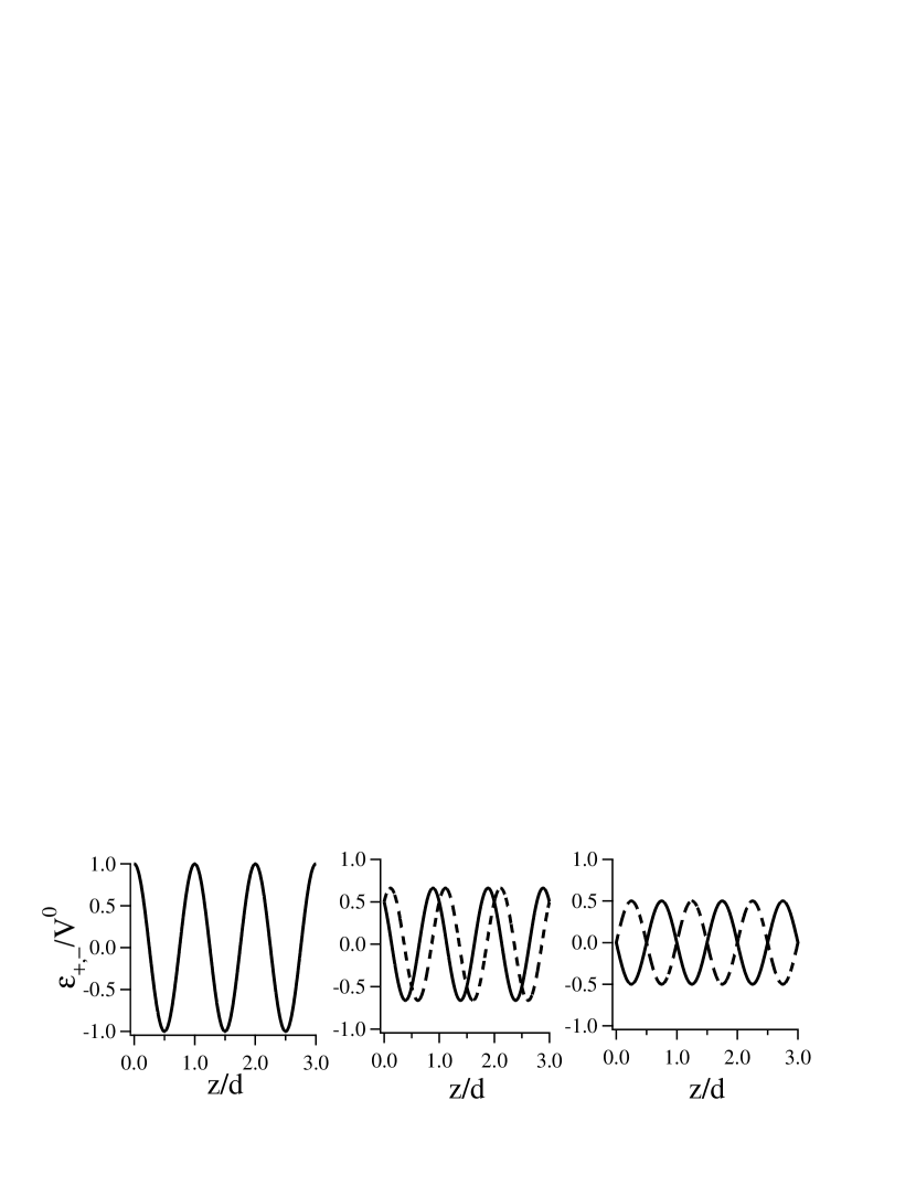
Figure 2: Eigenvalues $\epsilon_{+}$ (continuous line) and $\epsilon_{-}$ (dashed line), in units of $V^{0}$, plotted for different values of $\theta$ ($0$, $\pi/3$ and $\pi/2$ from left to right) in the case of the counterpropagating geometry corresponding to $\phi=\pi$ and for the value $\eta=-0.5$.

Fig. (2) reports the two eigenvalues of Eqs. (20) as a function of $z$ for different values of the relative angle $\theta$ between the two linear polarizations. The laser frequency is chosen such that $V^{1}=-0.5V^{0}$, that is $\eta=-0.5$. At $\theta=0$ with the laser polarizations parallel, $\epsilon_{+}$ and $\epsilon_{-}$ coincide. By increasing $|\theta|$, the minima of the potential curves $\epsilon_{+}$ and $\epsilon_{-}$ move in opposite directions along the $z$ axis, and the potential depth decreases. At $\theta=\pi/2$ the minima of $\epsilon_{+}$ coincide with the maxima of $\epsilon_{-}$, and their amplitudes are at the minimum. Let us suppose to start at $\theta=\pi/2$ preparing a $|+\rangle$ atom at the site $id$ and a $|-\rangle$ atom at the site $(i-\frac{1}{2})d$. Varying adiabatically $\theta$ from $\pi/2$ to $0$ (or to $\pi$) the two particle will occupy the same site. This protocol was used to transport the atoms from one site to the other in order to produce controlled collisions brennen99 ; jaksch99 ; mandel03 . We recall that in this counterpropagating geometry the effective magnetic field is oriented along the $z$ axis and is equal to zero for $\theta=0$, when the atoms collide.
Fig. 3 shows that the potential depth does not remain constant by varying $\theta$. As pointed in refs jaksch99 ; jaksch05a , this difficulty is avoided for a particular choice of the parameter $\eta$. In fact for $\eta^{2}=1$, the term $\cos^{2}\theta$ disappear in Eq. (25) and $U_{0}$ becomes a constant independent of $\theta$ and equal to $V^{0}$.

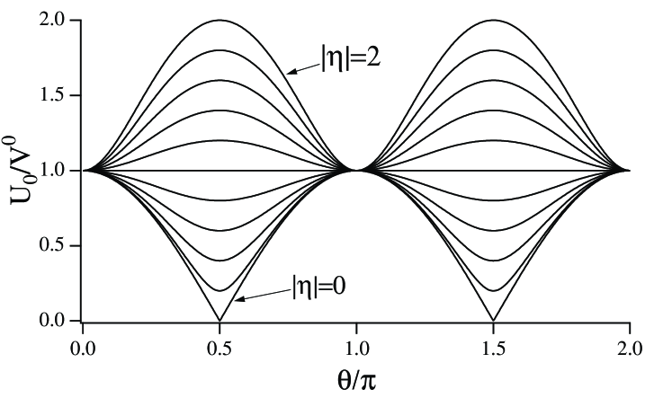
Figure 3: Potential depth $U_{0}$ as a function of $\theta$ for $|\eta|$ ranging between $0$ and $2$ in steps of $0.2$, from bottom to top. For $|\eta|=1$ the potential is a constant independent of $\theta$.

By assuming equal dipole moments for the D₁ and D₂ lines $\left|\langle J^{\prime}=\frac{1}{2}\left\|{\bf d}\right\|J=\frac{1}{2}\rangle\right|^{2}=\left|\langle J^{\prime}=\frac{3}{2}\left\|{\bf d}\right\|J=\frac{1}{2}\rangle\right|^{2}$note4 , the parameter $\eta(\omega)$ becomes:

$$\eta(\omega)=\frac{\Delta_{D2}-\Delta_{D1}}{\Delta_{D2}+2\Delta_{D1}}.$$ (26)

Fig. 4 reports the parameter $\eta$ versus the laser wavelength $\lambda$. The constraint $\eta^{2}=1$ implies $\eta=1$ or $\eta=-1$. The first condition is satisfied for $\Delta_{D1}=0$ which is not an acceptable value, since the whole treatment for the optical lattice potential is valid only for detunings $\Delta_{D1,2}$ large with respect to the typical hyperfine splitting. The $\eta=-1$ relation is satisfied if the laser wavelength is equal to the magic value $\lambda^{*}$

$$\frac{1}{\lambda^{*}}=\frac{1}{3}\left(\frac{1}{\lambda_{D1}}+\frac{2}{\lambda_{D2}}\right)$$ (27)

where $\lambda_{D1}$ and $\lambda_{D2}$ denote the resonant wavelengths for the D₁ and D₂ lines. For $\eta=-1$ the relative phase $\gamma_{0}$ becomes

$$\begin{split}\gamma_{0}&=\theta\quad\quad\quad\quad\,for\,\,0<\theta<\pi\\ \gamma_{0}&=2\pi-\theta\quad\quad for\,\,\pi\leq\theta\leq 2\pi\end{split}$$ (28)

Therefore for the magic wavelength $\lambda^{*}$ the potential depth is independent on $\theta$ and the phase $\gamma_{0}$ varies linearly with the relative angle $\theta$.

Figure 4: Plot of the dimensionless parameter $\eta^{2}$ as a function of the laser wavelength $\lambda$. The two continuous vertical lines denote the position of the resonant wavelengths $\lambda_{D2}$ and $\lambda_{D1}$, respectively. The dashed vertical line indicates the magic wavelength $\lambda^{*}$.

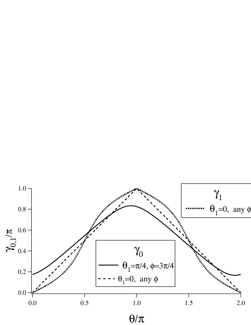
Figure 5: Optical lattice phase shifts $\gamma_{0}$ and $\gamma_{1}$ versus $\theta$ for the laser at the magic wavelength, corresponding to $\eta=-1$. For $\gamma_{0}$ the continuous line corresponds to $\theta_{1}=\pi/4$ and $\phi=3\pi/4$. The dashed line plots $\gamma_{0}$ at $\theta_{1}=0$ whichever value of $\phi$. The same $\gamma_{0}$ values are obtained for $\phi=\pi$ whichever value of $\theta_{1}$. For $\gamma_{1}$ the dotted line corresponds to $\theta_{1}=0$ whichever value of $\phi$. The coherent transport requires for the phase shift $\pi/2$ as initial value and $0$ as final value. A complete transport cannot be realized for the conditions corresponding to the continuous line, but instead can be realized for the dashed and dotted lines.

VI angle-tuned configuration

For $\phi$ different from $\pi$ the potential depth $U_{0}$ and the phase $\gamma_{0}$ depend on the angle $\theta_{1}$ as well. This reflects the fact that for $\phi\neq\pi$ the system is not invariant under rotations around the $z$ axis.
For the $U_{0}$ dependence on $\theta_{1}$ the magic wavelength $\lambda^{*}$ plays again a key role. In fact by choosing $\eta=-1$ Eqs. (21) reduce to

$$\begin{split}U_{0}&=V^{0}\;,\\ \gamma_{0}(\theta_{1},\theta,\phi)&=\arctan{\sqrt{\frac{1}{u^{2}}-1}}.\end{split}$$ (29)

Therefore the potential depth $U_{0}$ depends only on the laser wavelength.
The remaining dependence of $\gamma_{0}$ on the angles $(\theta_{1},\theta,\phi)$ defining the optical lattice represents a difficulty for the coherent transport operation. For instance for the values of $\theta_{1}=\pi/4$ and $\phi=3\pi/4$ the phase shift $\gamma_{0}$ versus $\theta$ is plotted as a dashed line in Fig. 5 and is compared to the value corresponding to the counterpropagating geometry, plotted as a continuous line. For those values of $\phi$ and $\theta_{1}$ the range of variation of $\gamma$ is smaller than $\pi$. This means that by varying $\theta$ the two potential curves corresponding to the two atomic eigenstates are shifted by a quantity smaller than the spatial period $d$. Thus the minima of the potentials for the two atomic eigenstates do not coincide and a complete transport is not realized. However under the special condition of $\theta_{1}=0$ Eq. (17) holds, and the phase $\gamma_{0}$ becomes

$$\begin{split}\gamma_{0}(\theta)&=\theta\quad\quad\quad\quad\,for\,\,0<\theta<\pi,\\ \gamma_{0}(\theta)&=2\pi-\theta\quad\quad for\,\,\pi\leq\theta\leq 2\pi.\end{split}$$ (30)

Therefore by choosing $\lambda=\lambda^{*}$ and $\theta_{1}=0$, the phase shift becomes fully equivalent to that of the counterpropagating case. Thus, it is possible to move the two potential curves of Eqs. (20) without changing the potential depth, and a spatial coherent transport with amplitude $d$ can be produced by varying the angle $\theta$ of the laser polarizations. For this angle-tuned configuration, even if the effective magnetic field is null at $\theta=0$ where the atoms collide, it includes a component along the $y$ axis at other values of $\theta$.

VII Transport of rubidium states

The vector component and the total potential of Eqs. (10) experienced by the atoms depend on the projection of the electron magnetic moment or, equivalently, of the total angular momentum ${\bf\hat{F}}$ along the local magnetic field. Different effective potentials are experienced by different Zeeman levels of the ground hyperfine state, and the laser parameters required for the coherent control depend on the atomic computational basis. Here we consider two different hyperfine-Zeeman states $|F,m_{F}\rangle$ of the ⁸⁷Rb atom as in the analysis of brennen99 ; jaksch99 ; mandel03 . As described in jaksch99 the potential experienced by the atoms in these internal states is derived from the potential of Eq. (10a) by considering the components of the electron spin for these states. However in the angle tuned geometry with $\phi\neq\pi$, the effective magnetic field also includes components oriented along the $x$ and $y$ axes. As a consequence the potential experienced by the atomic states depend on the optical lattice loading process and the occupation amplitudes for the Zeeman states. In fact Raman coherences of the type $|F,m\rangle\to|F^{\prime},m\pm 1\rangle$ are created by the effective magnetic field. As pointed out in ref. deutsch97 , in the tight binding regime where each lattice site can be considered as an independent potential well, the Wannier states constituting an orthonormal basis within each well in general become spinors.
For simplicity we analyze the case of an adiabatic loading of the $|F,m_{F}\rangle$ states in the lattice so that their $m_{F}$ component is oriented along the local magnetic field ${\bf B}_{\mathrm{eff}}$. Thus we impose the atomic states under consideration to be the $|F,m_{F}\rangle$ eigenstates along the local magnetic field. Let’s consider the following states:

$$\begin{split}|0>&=|F=2,m_{F}=2\rangle=|I=\frac{3}{2},m_{I}=\frac{3}{2}\rangle|S,m_{S}=\frac{1}{2}\rangle\,,\\ |1>&=|F,m_{F}\rangle\,=c_{+}|I=\frac{3}{2},m_{I}=m_{F}-\frac{1}{2}\rangle|S,m_{S}=\frac{1}{2}\rangle+c_{-}|I=\frac{3}{2},m^{\prime}_{I}=m_{F}+\frac{1}{2}\rangle|S,m_{S}=-\frac{1}{2}\rangle\,,\\ \end{split}$$ (31)

the coefficients $c_{\pm}$ defining the normalized superposition. For the $|F,m_{F}=1\rangle$ state of the explorations in refs. brennen99 ; jaksch99 ; mandel03 the coefficients are $c_{+}=1/2$ and $c_{-}=\sqrt{3}/2$. The energies $E_{0,1}$ of the states $|0,1\rangle$ at a fixed position $z$ within the optical lattice are given by

$$\begin{split}E_{0}\left(\theta_{1},\theta,\phi,z\right)&=\epsilon_{+}\left(\theta_{1},\theta,\phi,z\right)=U_{0}\cos(2\pi\frac{z}{d}+\gamma_{0})\,,\\ E_{1}\left(z,\theta_{1},\theta,\phi\right)&=|c_{+}|^{2}\epsilon_{+}\left(\theta_{1},\theta,\phi,z\right)+|c_{-}|^{2}\epsilon_{-}\left(\theta_{1},\theta,\phi,z\right)=V^{0}u\cos(2\pi\frac{z}{d})+V^{1}b\left(|c_{+}|^{2}-|c_{-}|^{2}\right)\sin(2\pi\frac{z}{d})\\ &=U_{1}\cos(2\pi\frac{z}{d}-\gamma_{1}).\\ \end{split}$$ (32)

While $U_{0}$ and $\gamma_{0}$ are given by Eq. (21), the potential depth $U_{1}(\theta_{1},\theta,\phi)$ and the phase $\gamma_{1}(\theta_{1},\theta,\phi)$ are given by

$$U_{1} =V^{0}\sqrt{\eta^{2}\Delta^{2}_{c}+(1-\eta^{2}\Delta^{2}_{c})u^{2}},$$ (33a)

$$\gamma_{1} =-\arctan\left(\eta\Delta_{c}\sqrt{\frac{1}{u^{2}}-1}\right)\,,$$ (33b)

where

$$\Delta_{c}=|c_{-}|^{2}-|c_{+}|^{2}.$$ (34)

We obtain two different effective lattice potentials trapping the atoms in the$|0\rangle$ and $|1\rangle$ hyperfine-Zeeman states.
Because Eqs. (33) have the same structure as Eqs. (29), the coherent transport is determined by the $u(\theta)$ dependence at fixed values $\theta_{1}$ and $\phi$. By using this analogy we conclude that, in order to perform a controlled-collisions experiment, the potentials seen by the two hyperfine states $|0,1\rangle$ must move in opposite direction when $\theta$ is varied. The comparison Eq. (33b) to Eq. (21b) indicates that this condition is satisfied when the $|1\rangle$ state is chosen such that $\Delta_{c}>0$, that is, when $|c_{-}|>|c_{+}|$. For the states $|F=2,m_{F}=-2\rangle$, $|F=2,m_{F}=-1\rangle$, $|F=1,m_{F}=1\rangle$ this inequality is satisfied.

The optimal coherent transport is obtained when the potential depth is constant by varying the $\theta$ control parameter. In Section V the constance of the optical depth was realized by fixing the laser wavelength at the magic value. For the present case of two hyperfine states a unique magic wavelength where the $U_{0}$ and $U_{1}$ potential depths are both independent of $\theta$ does not exist. While the $U_{0}$ constance imposes $\eta^{2}=1$ and produces the magic wavelength Eq. (27), the $U_{1}$ constance imposes $\left(\eta\Delta_{c}\right)^{2}=1$ leading to a different laser wavelength. For instance, at $\theta_{1}=0$ and fixing the laser wavelength to the $\lambda^{*}$ value of Eq. (27) such that $\eta=-1$, the potential depths for the $|0,1\rangle$ states become

$$\begin{split}U_{0}&=V^{0}\,,\\ U_{1}(\theta)&=V^{0}\sqrt{\Delta_{c}^{2}+(1-\Delta_{c}^{2})\cos^{2}\theta},\end{split}$$ (35)

while their phases $\gamma_{0,1}$ are

$$\begin{split}\gamma_{0}(\theta)&=\theta\,,\\ \gamma_{1}(\theta)&=\arctan\left(\Delta_{c}\tan\theta\right).\end{split}$$ (36)

When $\theta$ is varied from $\frac{\pi}{2}$ to $0$ or $\pi$, while the $U_{0}$ potential depth is independent of $\theta$, the $U_{1}$ potential depth depends on $\theta$ and its range is determined by $\Delta_{c}$, whence by the $c_{\pm}$ values. Therefore, when $\theta$ is varied the potentials experienced by the $|0,1\rangle$ states move with different velocities. The phase $\gamma_{0}$ is linearly dependent of $\theta$, while the dependence of $\gamma_{1}$ on $\theta$ has a more complicated behavior. For the case of the $|F=1,m_{F}=1\rangle$ state the $\gamma_{1}$ dependence is shown by the dotted line in Fig. 5. The coherent transport condition of phase shifts $\gamma_{0,1}$ varying from $\pi/2$ to $0$ is realized for both the hyperfine-Zeeman states. Different results for the change in the potential depth and for the phase dependence on $\theta$, and therefore for the displacements of the two potentials, are obtained for a laser wavelength different from the magic one.

VIII Adiabatic transport

In order to realize an efficient quantum gate, the time dependence of polarization angle $\theta$ should be chosen so that the transport of the atomic states is realized in the adiabatic limit, i.e. the atoms remain in the ground state of local optical potential. For an analysis of the adiabaticity constraint necessary for the coherent transport we approximate the atomic potential of Eq. (20) with a harmonic one. For non interacting atoms experiencing a harmonic potential moving with respect to the laboratory frame, the Hamiltonian may be written as salomon97

$$H=\frac{p^{2}}{2m}+\frac{1}{2}m\Omega^{2}z^{2}+M\ddot{z}_{hp}(t)z,$$ (37)

where $z$ denotes the coordinate of the atom in the harmonic potential frame, $\ddot{z}_{hp}$ represents the acceleration of the harmonic potential in the laboratory frame, and the oscillation frequency $\Omega$ of the harmonic oscillator is

$$\Omega=\sqrt{\frac{U_{0}}{M}}\frac{4\pi}{\lambda}sin(\phi/2).$$ (38)

If we consider the last term of the above Hamiltonian as a time-dependent perturbation, the probability of transferring an atom to the first excited level of the harmonic potential is

$$P_{f,i}=\frac{1}{2a_{ho}^{2}\Omega^{2}}\left|\int_{0}^{T}\ddot{z}_{hp}(t)e^{i\Omega t}dt\right|^{2},$$ (39)

where $a_{ho}=\sqrt{\hbar/M\omega}$ is the ground state radius for the harmonic potential, and $T$ is the time required for the coherent transport process.
The amplitude of the transfer probability of Eq. (39) depends greatly on the time dependence of the $\ddot{z}_{hp}$ acceleration. At first we will suppose that, as in the theoretical analysis of ref. jaksch99 and in the experimental investigation of ref.mandel03 , the potential moves at a constant speed, by imposing an infinite acceleration at $t=0$ and $t=T$. For this transformation the adiabatic condition for the atomic transformation requires

$$T\gg\frac{d}{a_{ho}}\frac{1}{\Omega}=\frac{1}{2}\left(\frac{\lambda^{6}M^{3}}{(4\pi)^{2}\hbar^{2}U_{0}}\right)^{1/4}sin\left(\phi/2\right)^{-\frac{3}{2}}.$$ (40)

Owing to this dependence on $\phi$, for a constant speed of the potential the time $T$ required to realize an adiabatic coherent transport in the angle-tuned configuration is much longer than in the counterpropagating case, for a given depth of the optical potential . Such result could impose a strong constraint for performing quantum computation with angle-tuned lattices.
However, the condition on $T$ for realizing the adiabatic limit becomes less restrictive if we assume a different motion for the lattice harmonic potential confining the atoms. For instance, let us assume that the lattice is constantly accelerated from $t=0$ to $t=\frac{T}{2}$ and constantly decelerated from $t=\frac{T}{2}$ to $t=T$. Thus the adiabatic condition becomes

$$T\gg\sqrt{\frac{d}{a_{ho}}}\frac{1}{\Omega}=\frac{1}{\sqrt{2}}\left(\frac{\lambda^{10}M^{5}}{(4\pi)^{6}\hbar^{2}U_{0}^{3}}\right)^{1/8}sin\left(\phi/2\right)^{-\frac{5}{4}}.$$ (41)

Therefore using this motion of the potential, the dependence of the minimum time for the coherent transport on the angle $\phi$ is modified causing a decrease in the time by a factor which for $\phi\sim 5^{\circ}$ is larger than 2. Moreover the additional dependence on $\lambda$, $U_{0}$, and the physical constants of Eq. (41) contributes to the decrease of the time scale, so that for the experimental conditions of ref. mandel03 transport times around 10 $\mu$s can be achieved.

IX Conclusions

In quantum computation experiments with neutral atoms loaded in optical lattices, a crucial aspect is the single site addressability. In the angle-tuned configuration where the lattice constant could be large, the question of the single site addressability is shifted to a frame of more accessible dimensions. For this geometry the coherent transport protocol requires specific conditions of the laser beam polarizations, linked to the breaking of the rotational symmetry associated to the counterpropagating geometry. An additional request is the constance of the optical potential depth during the coherent transport. This constance is realized by choosing a magic wavelength for the laser fields producing the lattice. The value of the magic wavelength is independent of the lattice geometry. However an unique magic wavelength for the transport of all hyperfine-Zeeman atomic states does not exist.

Coherent transport within an optical lattice represents a component of the process based on ultracold collisions and leading to entanglement of neutral atoms and implementation of quantum logic. By storing the ultracold atoms in the microscopic potentials provided by optical lattices the collisional interactions can be controlled via laser parameters. At the low temperature associated to the Mott insulator, the collisional process is described through s-wave scattering. In the $\theta_{1}=0$ laser configuration of the angle-tuned geometry, at $\theta=0$ the effective magnetic field is null and the scattering potentials associated to the different atomic states have an identical spatial dependence. However, as new feature brought by the angle-tuned geometry, at $\theta\neq 0$ the effective magnetic field is different from zero and oriented along different directions for different hyperfine-Zeeman states. Therefore during the whole collisional process the colliding atoms may be oriented along different spatial directions. In order to treat this collisional configuration, the atomic interaction may be described through the pseudopotential models introduced in refs. bolda03 ; stock05 for asymmetric trap geometries.

The atomic control is based on a the realization of a Mott insulator phase, in which the number of atoms occupying each lattice site is fixed. The physics of such a system is described in terms of a Bose-Hubbard model whose Hamiltonian contains the on-site repulsion resulting from the collisional interactions between the atoms, and the hopping matrix elements that take into account the tunneling rate of the atoms between neighboring sites. Both the repulsive interaction and the hopping energy can be tuned by adjusting the lasers setup, as reviewed in jaksch05b . The Mott insulator phase is realized under precise conditions between the on-site repulsion and the hopping matrix elements. The dependence of these parameters defining the angle-tuned lattice should be investigate in order to realize a Mott insulator in an angle tuned geometry.

X Acknowledgments

This researach was financially supported by the EU through the STREP Project OLAQUI and by the Italian MIUR through a PRIN Project. The authors are gratefully to Dieter Jaksch and Carl J. Williams for useful discussions.

References

- (1) I. Bloch, J. Phys. B: At. Mol. Opt. Phys. 38, S629-S643 (2005).
- (2) V. Finkelstein, P.R. Berman, and J. Guo, Phys. Rev. A 45, 1829 (1992).
- (3) R. Taïeb, P. Marte, R. Dum, and P. Zoller, Phys. Rev. A 47, 4986 (1993).
- (4) S. Marksteiner, R. Walser, P. Marte and P. Zoller, Appl. Phys. B. 60, 145 (1995).
- (5) G. K. Brennen, C. M. Caves, P. S. Jessen, and I. H. Deutsch, Phys. Rev. Lett. 82, 1060 (1999).
- (6) D. Jaksch, H.-J. Briegel, J. I. Cirac, C. W. Gardiner, and P. Zoller, Phys. Rev. Lett. 82, 1975 (1999).
- (7) D. Jaksch, Comtp. Phys. 45, 367-381 (2004).
- (8) O. Mandel, M. Greiner, A. Widera, T. Rom, T.W. Hänsch and I. Bloch, Phys. Rev. Lett. 91, 010407 (2003).
- (9) S. Friebel, C. D’Andrea, J. Walz, M. Weitz, and T.W. Hänsch, Phys. Rev. A 57, R20, (1998).
- (10) O. Morsch, J.H. Müller, M. Cristiani, D. Ciampini, and E. Arimondo, Phys. Rev. Lett. 87, 140402 (2001).
- (11) M. Albiez, R. Gati, J. Fölling, S. Hunsmann, M. Cristiani, and M.K. Oberthaler, Phys. Rev. Lett. 95, 010402 (2005)
- (12) Z. Hadzibabic, S. Stock, B. Battelier, V. Bretin, and J. Dalibard, Phys. Rev. Lett. 93, 180403 (2004).
- (13) L. Fallani, C. Fort, J.E. Lye, and M. Inguscio, Opt. Express 13, 4303 (2005).
- (14) H. Moritz, T. Stöferle, M. Köhl, and T. Esslinger, Phys. Rev. Lett. 91, 250402 (2003).
- (15) I. H. Deutsch and P. S. Jessen, Phys. Rev. A 57, 1972 (1998).
- (16) Owing to this transformation the angle between the polarizations of the lin--lin geometry is
- (17) The atomic motion is determined also by the gravitational and trapping potentials not included here.
- (18) C.Y. Park et al, Phys. Rev. A 63 032512 (2001) and 65 033410 (2002).
- (19) does not have the dimensions of a magnetic field. The correct magnetic field is , with the Bohr magneton.
- (20) On the basis of the lifetime measurements of volz96 the ratio of the dipole moments for the D2 and D1 is 1.027(1).
- (21) U. Volz and H. Schmoranzer, Physica Scripta T65, 48 (1996).
- (22) I.H. Deutsch, J. Grondalski, and P.M. Alsing, Phys. Rev. A 56, R1705 (1997).
- (23) E. Peik, M. Ben Dahan, I. Bouchoule, Y. Castin, and C. Salomon, Phys. Rev. A 55, 2989 (1997).
- (24) E. L. Bolda, E. Tiesinga, and P. S. Julienne, Phys. Rev. A 68, 032702 (2003).
- (25) R. Stock, A. Silberfarb, E. L. Bolda, and I.H. Deutsch, Phys. Rev. Lett. 94, 023202 (2005).
- (26) D. Jaksch and P. Zoller, Ann. Phys. 315, 52 (2005), and references therein.