Single-Species Three-Particle Reactions in One Dimension

Abstract

Renormalization group calculations for fluctuation-dominated reaction-diffusion systems are generally in agreement with simulations and exact solutions. However, simulations of the single-species reactions $3A\to(\emptyset,A,2A)$ at their upper critical dimension $d_{c}=1$ have found asymptotic densities argued to be inconsistent with renormalization group predictions. We show that this discrepancy is resolved by inclusion of the leading corrections to scaling, which we derive explicitly and show to be universal, a property not shared by the $A+A\to(\emptyset,A)$ reactions. Finally, we demonstrate that two previous Smoluchowski approaches to this problem reduce, with various corrections, to a single theory which surprisingly yields the same asymptotic density as the renormalization group.

I Introduction

Reaction-diffusion systems are known to be strongly dependent on fluctuations when the spatial dimension $d$ is at or below an upper critical dimension $d_{c}$. This fluctuation-dominated case has been treated by field-theoretic renormalization group (RG) methods for a wide variety of reaction types and conditions, as recently reviewed Täuber et al. (2005). Comparison of the RG results with exact solutions and simulations has generally yielded agreement or at least consistency, as detailed in examples given below. However, simulations of the single-species $3A\to(\emptyset,A,2A)$ reactions at the upper critical dimension $d=d_{c}=1$ ben Avraham (1993); Oshanin et al. (1995) appear to be inconsistent with RG predictions Lee (1994). This discrepancy is noteworthy since these reactions present one of the simplest and directly testable cases. In the current work we demonstrate that there is no discrepancy.

The general single-species reaction-diffusion decay $kA\to\ell A$ with integers $\ell<k$ has an upper critical dimension $d_{c}=2/(k-1)$. Above the upper critical dimension the density $n(t)$ follows the rate equation, $\partial_{t}n=-\lambda n^{k}$, which gives the asymptotic decay $n\sim t^{-1/(k-1)}$ with an amplitude that depends on the nonuniversal rate constant $\lambda$. Below the upper critical dimension particle anti-correlations neglected by the rate equation become relevant, giving rise to a slower decay $n\sim A_{k,\ell}(Dt)^{-d/2}$, with $A_{k,\ell}$ a universal constant dependent only on the reaction type ($k$ and $\ell$) and the dimension $d$. RG methods have been used to show the exponent to be exact Peliti (1986), and to demonstrate the universality of $A_{k,\ell}$ and provide an expansion in powers of $d_{c}-d$ for the amplitude Lee (1994).

The amplitude expansion may be tested by comparison with exact solutions and simulations. For example, solvable realizations of the $A+A\to 0$ model in one dimension give the decay amplitude of $A_{2,0}=1/\sqrt{8\pi}\simeq 0.199$ Bramson and Griffeath (1980); Lushnikov (1987). The RG expansion in $\epsilon=d_{c}-d=1$ gives instead $A_{2,0}\simeq 0.080+0.029+\dots$ Lee (1994). Evidently the truncated perturbative RG is of little accuracy when $\epsilon=1$. However, if the diffusive transport is replaced by long-range hops, the upper critical dimension can be continuously lowered from two to one, allowing for a truly small $\epsilon$ in spatial dimension $d=1$ Vernon (2003). In this case, the theoretical amplitude compares well with simulations. Also noteworthy is that the ratio $A_{2,1}/A_{2,0}=2$ found from exact solutions Bramson and Griffeath (1980); Bramson and Lebowitz (1988) is also an exact result from the RG calculation, i.e., a field rescaling transformation in the field theory shows this ratio to hold to all orders in the $\epsilon$ expansion Lee (1994). Thus simulations and exact solutions for $d<d_{c}$ are in general agreement with the field-theoretic RG approach.

For the borderline case of $d=d_{c}$, the density is predicted to decay with the rate equation exponent, but with logarithmic corrections and a universal amplitude Lee (1994),

$$n\sim A_{k,\ell}\left(\frac{\ln t}{Dt}\right)^{1/(k-1)}.$$ (1)

The amplitude in this case is given explicitly, rather than perturbatively, as

$$A_{k,\ell}=\left(\frac{k^{(k-2)/(k-1)}(k-2)!}{4\pi(k-\ell)}\right)^{1/(k-1)}.$$ (2)

This explicit result provides then a strong test for the RG calculation. An exact solution is available for a particular realization of the $A+A\to(\emptyset,A)$ reactions in $d=d_{c}=2$ Bramson and Griffeath (1980), with values $A_{2,0}=1/8\pi$ and $A_{2,1}=1/4\pi$ that match the RG results, eq. (2).

However, the predictions for the $3A\to\ell A$ reactions at the upper critical dimension $d_{c}=1$ have been the source of some controversy. Simulations have demonstrated logarithmic corrections in $d=1$, but with amplitudes that differ from the renormalization group predictions. Specifically, while eq. (2) gives $A_{3,\ell}\simeq 0.21$, $0.26$, and $0.37$ for $\ell=0$, $1$, and $2$ respectively, simulations have reported values $A_{3,0}\simeq 0.26$ Oshanin et al. (1995), $A_{3,1}\simeq 0.76$, and $A_{3,2}\simeq 0.93$ ben Avraham (1993). Further, the $3A\to\emptyset$ simulations were found to be consistent with a version of Smoluchowski theory adapted for three-particle reactions Oshanin et al. (1995). That is, an approximate theory appears to agree better with the simulations than the RG calculation, which in principle involves no approximations.

To address this discrepancy, we revisit all of the field-theoretic approach, simulations, and Smoluchowski theory. Our main results are as follows. First, we demonstrate with RG methods that the leading corrections to the asymptotic density are universal, a surprising property not shared by the $A+A\to(\emptyset,A)$ reactions at their upper critical dimension $d_{c}=2$. Our result is

$$n(t)\sim A_{3,\ell}\left(\frac{\ln t}{Dt}\right)^{1/2}+B_{3,\ell}\left(\frac{1}{Dt}\right)^{1/2}+O\left(\frac{1}{\sqrt{Dt\ln t}}\right)$$ (3)

with $A_{3,\ell}$ given by eq. (2) and $B_{3,\ell}$ computed in section II below. Explicitly,

$$A_{3,\ell}=\left(\frac{\sqrt{3}}{4\pi(3-\ell)}\right)^{1/2},\qquad B_{3,\ell}=\frac{9\sqrt{2\pi}(2+\ell)}{128}$$ (4)

The next term in the expansion is nonuniversal.

This universal leading correction is quite significant in the time range available to simulations, of the order of half the magnitude of the asymptotic density. Consequently, including this term makes the RG predictions consistent with the previous $3A\to\emptyset$ simulations Oshanin et al. (1995) but not with the $3A\to(A,2A)$ simulations ben Avraham (1993).

This motivated us to conduct our own simulations, which are presented in section III. Our simulation data is consistent with that of Ref. Oshanin et al. (1995) for the $3A\to\emptyset$ reaction, but not compatible with the data of Ref. ben Avraham (1993) for the $3A\to(A,2A)$ reactions, which we believe to be in err. Our simulation data is not capable of directly confirming the predicted amplitudes due to remaining, slow transients. However, the data shows no discrepancy with the RG predictions for all three cases.

In order to have a test of the RG predictions that does not contain slow transients, we turn in section IV to the field rescaling transformation in the field theory, which we use to predict relations between pure and mixed reactions. Our simulations verify that these relations hold with high accuracy.

Finally, we turn to the Smoluchowski approach, which is presented in section V. We begin by demonstrating that the Smoluchowski solution for the $A+A\to(\emptyset,A)$ reactions in $d=2$ not only exhibits the logarithmic corrections, but also gives the correct density amplitude $A_{2,\ell}$. We believe this to be a new result. This is also germane to the $3A\to\ell A$ reaction in $d=d_{c}=1$ because both Smoluchowski approaches to this problem in the literature Krapivsky (1994); Oshanin et al. (1995) are constructed via a quasi-two-dimensional approach. We show that these two approaches, when various omitted factors are included, reduce to the same Smoluchowski theory, and further that this theory reproduces the same asymptotic density as the RG approach.

A summary is presented in section VI.

II Renormalization Group Calculation

Our presentation in this section will follow closely the formalism developed in Lee (1994). The Doi-Peliti mapping of reaction-diffusion systems to a field theory is by now a standard technique Täuber et al. (2005); Doi (1976); Peliti (1985), giving for the $3A\to\ell A$ reaction the action

$$S=\int d^{d}x\,dt\Bigl{[} \bar{\phi}(\partial_{t}-D\nabla^{2})\phi+c_{1}\lambda_{0}\bar{\phi}\phi^{3}+c_{2}\lambda_{0}\bar{\phi}^{2}\phi^{3}$$ (5)

$$+\lambda_{0}\bar{\phi}^{3}\phi^{3}-n_{0}\bar{\phi}\,\delta(t)\Bigr{]}.$$

The first term in the integrand corresponds to the diffusion process and provides the propagator for the field theory. The higher order terms correspond to the reaction and provide vertices in the diagrammatic expansion. The Poisson initial conditions are reflected in the initial term $n_{0}\bar{\phi}(t=0)$.

Here $\lambda_{0}$ is a nonuniversal, bare coupling constant associated with the microscopic reaction rate, while the coefficients $c_{1}$ and $c_{2}$ depend only on $\ell$. These coefficients are determined by a field shift: the Doi-Peliti mapping first gives the action in terms of fields $\hat{\phi}$ and $\phi$, with the coupling terms $\lambda_{0}(\hat{\phi}^{3}-\hat{\phi}^{\ell})\phi^{3}$. To eliminate a “final term” $\phi(t_{f})$ that complicates the calculations (see Lee (1994); Täuber et al. (2005) for details) the field shift $\hat{\phi}=1+\bar{\phi}$ is then employed, resulting in the coupling terms in eq. (5), with the coefficients

$$c_{1}=3-\ell,\qquad c_{2}={\textstyle\frac{1}{2}}(3-\ell)(2+\ell).$$ (6)

The renormalization of this action Täuber et al. (2005); Lee (1994), necessary to obtain finite calculations for $d\leq 1$, is relatively straightforward, requiring only renormalization of the coupling constant. An arbitrary normalization time $t_{0}$ is used to define a dimensionless, renormalized coupling constant $g_{R}$. The renormalization group flow, for $t\gg t_{0}$, is described by the Callan-Symanzik equation

$$n(t,n_{0},g_{R},t_{0})=(t_{0}/t)^{d/2}n\bigl{(}t_{0},\tilde{n}_{0}(t),\tilde{g}_{R}(t),t_{0}\bigr{)}$$ (7)

with the running initial density

$$\tilde{n}_{0}(t)=n_{0}(t/t_{0})^{d/2}$$ (8)

and running coupling for $d=d_{c}=1$ given by

$$\tilde{g}_{R}(t)\sim\frac{2\pi}{\sqrt{3}\ln(t/\tau)}$$ (9)

where $\tau$ is some nonuniversal time constant related, via the diffusion constant, to the short distance cutoff of the field theory. The coefficient in eq. (9) is determined by the loop integrals in the definition of the renormalized coupling constant. The logarithmic time dependence is characteristic of marginal operators at the upper critical dimension.

A loop expansion in terms of the bare coupling $\lambda_{0}$ and initial density $n_{0}$ is used for the right hand side of eq. (7) to give the asymptotic $t\gg t_{0}$ density. For example, the tree-level (zero loop) diagrams may be summed by a Dyson equation Lee (1994), giving

$$n^{(0)}(t)=\frac{n_{0}}{(1+2n_{0}^{2}c_{1}\lambda_{0}t)^{1/2}}\sim(2c_{1}\lambda_{0}t)^{-1/2}$$ (10)

The coupling $\lambda_{0}/D$ is converted to $g_{R}$ and then replaced by the running coupling $\tilde{g}_{R}$. The initial density $n_{0}$ is replaced by $\tilde{n}_{0}$, which grows as $t^{d/2}$ via eq. (8). This latter step allows us to keep only the large $n_{0}$ limit in the unrenormalized density calculation. Any corrections due to finite $n_{0}$ will renormalize to subasymptotic contributions to the density. Finally, the time is set to $t_{0}$ and the prefactor in eq. (7) is included, giving the renormalized contribution

$$n^{(0)}_{R}(t)\sim\frac{(t_{0}/t)^{1/2}}{(2c_{1}\tilde{g}_{R}Dt_{0})^{1/2}}\sim\left(\frac{\sqrt{3}\ln t}{4\pi c_{1}Dt}\right)^{1/2}.$$ (11)

The higher order diagrams give renormalized contributions at order $(Dt)^{-1/2}\tilde{g}_{R}^{(m-1)/2}$, where $m$ is the number of loops. Since $\tilde{g}_{R}\sim 1/\ln t$ for large $t$, these represent subleading terms to the asymptotic density. Thus with eq. (6) for $c_{1}$ we obtain the leading order asymptotic density reported in Lee (1994), and given by eq. (1).

Up to this point we have summarized results from Lee (1994). Now we demonstrate that the leading corrections to the asymptotic density are themselves universal. The renormalized loop expansion with $\tilde{g}_{R}\sim 1/\ln(t/\tau)$ takes the form

$$(Dt)^{1/2}n(t)=A\sqrt{\ln(t/\tau)}+B+C/\sqrt{\ln(t/\tau)}+\dots$$ (12)

where $A$, $B$, $C$, … are universal coefficients. Nonuniversal terms, apart from $\tau$ above, are suppressed by negative powers of time. Reorganizing the expansion in terms of $\ln t$ via $\sqrt{\ln(t/\tau)}\sim\sqrt{\ln t}+\frac{1}{2}\ln\tau/\sqrt{\ln t}+\dots$, we observe that the nonuniversal $\tau$ dependence does not enter until order $1/\sqrt{\ln t}$. Hence, $B_{3,\ell}$ represents a universal leading correction to the asymptotic density.

This is in contrast to the $A+A\to(\emptyset,A)$ reaction at the upper critical dimension, for which the renormalized loop expansion has the form $(Dt)^{-1}[A\ln(t/\tau)+B+\dots]$, and the $\tau$ dependence enters the leading correction.

Next we determine the coefficient. As presented in Lee (1994), the summation of all one-loop diagrams requires the use of the tree-level density $n^{(0)}(t)$, given by eq. (10), and the tree-level response function $G^{(0)}(x,t_{1},t_{2})=\langle\phi(x,t_{2})\bar{\phi}(0,t_{1})\rangle_{0}$, where the subscript on the angle brackets indicates a tree-level average. With the Fourier transform $f(p)=\int dx\,e^{-ipx}f(x)$ we obtain

$$G^{(0)}(p,t_{1},t_{2})\sim\left(\frac{t_{1}}{t_{2}}\right)^{3/2}e^{-Dp^{2}(t_{2}-t_{1})}$$ (13)

in the large $n_{0}$ limit, which is sufficient for our purposes. From Lee (1994) the one-loop diagram contribution is given by

$$n^{(1)}(t)=6\int_{0}^{t}dt_{2}\int_{0}^{t_{2}}dt_{1}\int{dp\over 2\pi}G^{(0)}(0,t,t_{2})(-c_{1}\lambda_{0})n^{(0)}(t_{2})G^{(0)}(p,t_{2},t_{1})G^{(0)}(-p,t_{2},t_{1})(-c_{2}\lambda_{0})[n^{(0)}(t_{1})]^{3}$$ (14)

The factor of six results from the combinatorics of attaching the response functions to the vertices. Evaluating eq. (14) and using the result in the right-hand side of the CS equation (7) gives the one-loop contribution

$$n_{R}^{(1)}(t)\sim\frac{9\sqrt{2\pi}c_{2}}{64c_{1}}(Dt)^{-1/2}$$ (15)

Substituting for $c_{1}$ and $c_{2}$ via eq. (6) gives the value for $B_{3,\ell}$ reported in eq. (4).

III Simulations

In order to test our density calculations, we simulate the $3A\to(\emptyset,A,2A)$ reactions in one dimension. We employ synchronous dynamics, in which the particles are restricted to be on all even or all odd numbered sites at a given time. All particles are updated simultaneously, each particle randomly hoping one site left or right, which corresponds with a lattice spacing of unity to a diffusion constant $D=1/2$. Subsequent reactions occur between particles on the same site until there are no more than two particles per site. This completes a single time step.

For initial conditions, each lattice site is randomly assigned 0, 1, or 2 particles with probabilities $p_{0}$, $p_{1}$, and $p_{2}$ respectively. We choose the $p_{i}$ as follows: first, the particle numbers are determined by a Poisson distribution with average $n_{0}$. Then these particles are allowed to react until there are no more than two particles per site, which gives the site occupation probabilities ($p_{0}$, $p_{1}$, $p_{2}$) as functions of $n_{0}$ and $\ell$. In order to reduce initial density transients, we then take the limit $n_{0}\to\infty$, which gives

$$(p_{0},p_{1},p_{2})=\cases{\textstyle(\frac{1}{3},\frac{1}{3},\frac{1}{3})&$\ell=0$\cr(0,\frac{1}{2},\frac{1}{2})&$\ell=1$\cr(0,0,1)&$\ell=2$.}$$ (16)

These probabilities are used as the initial conditions for our simulations. All simulations were conducted on a lattice of size $2^{23}\simeq 8.4\times 10^{6}$ for $10^{8}$ time steps, with 10 to 20 independent runs for each case.

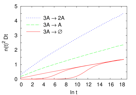
Figure 1: Plot of $n(t)^{2}Dt$ versus $\ln t$ for the $3A\to(\emptyset,A,2A)$ reactions, as labeled. The three curves for the $3A\to\emptyset$ reaction correspond, from top to bottom, to initial densities $n_{0}\to\infty$, $n_{0}=0.1$ and $n_{0}=0.01$. The rate equation prediction $n~{}\sim t^{-1/2}$ would correspond to a horizontal line.

In Fig. 1 we show the densities for the three reactions, plotted as $n(t)^{2}Dt$ versus $\ln t$. The data are clearly inconsistent with the rate equation result, $n\sim t^{-1/2}$, suggesting logarithmic corrections. According to eq. (1) the density plotted with these axes should approach a straight line with slope $A_{3,\ell}^{2}$. While the data show seemingly little curvature at late times, we present evidence below that suggests the asymptotic slopes have not been reached.

Also illustrated in Fig. 1 is the universality with respect to the initial density, shown for the $3A\to\emptyset$ reaction. Initial densities of $n_{0}=0.1$ and $n_{0}=0.01$ produce only transient deviations from the $n_{0}\to\infty$ data. The duration of the transient grows with decreasing $n_{0}$.

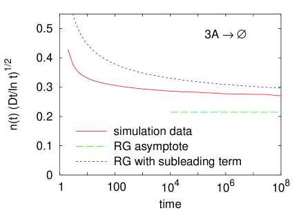
Figure 2: Plot of the density scaled by its expected time dependence versus time for the $3A\to\emptyset$ reaction. The data is averaged over 20 independent runs. Also shown are the RG predictions for the asymptote, a constant on this plot, and the asymptote with universal leading corrections.

Next we show, in turn, the same data for each of the pure reactions, as compared to the RG predictions. In Fig. 2, the density is multiplied by $\sqrt{Dt/\ln t}$, the inverse of the expected time dependence, and this is plotted versus time. According to the RG prediction, the data should approach the constant value $A_{3,0}$ asymptotically. This value included on the plot, and is seen to be well below the data. Also plotted is the universal sum of the asymptotic density and leading corrections. It is clear the leading corrections play a significant role in the time range accessible to simulation. It is important to note that the upper RG curve has the lower constant as its asymptote.

Our simulations appear to be consistent with those of Ref. Oshanin et al. (1995). We further conclude that the simulations are not in conflict with the RG calculations. The slow, logarithmic decay of the nonuniversal transient is responsible for the remaining discrepancy between the simulation data and the RG. Extending the simulations to asymptotia would appear to be impossible.

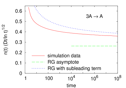
Figure 3: Plot of the $3A\to A$ simulation data, with axes and RG predictions as described in Fig. 2. The data is averaged over 15 independent runs.

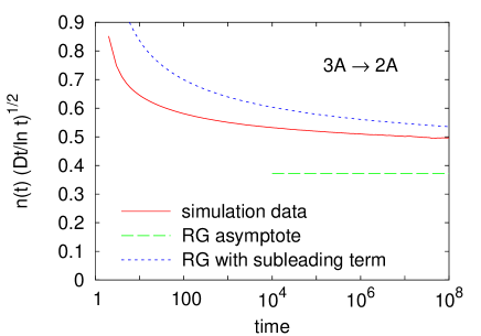
Figure 4: Plot of the $3A\to 2A$ simulation data, with axes and RG predictions as described in Fig. 2. The data is averaged over 10 independent runs.

Similar plots for the $\ell=1$ and $\ell=2$ reactions are shown in Figs. 3 and 4. In each case, the data fall well above the RG asymptote, but below the RG asymptote with the universal leading corrections. Here we note, observing the vertical scale, that our data are not consistent with the amplitudes 0.76 ($\ell=1$) and 0.93 ($\ell=2$) reported in ben Avraham (1993).

IV Mixed Reactions and the Field Rescaling Transformation

The RG field rescaling transformation, described below, predicts relationships between various mixed and pure reactions, similar to the predicted amplitude ratio for the $k=2$ case. These predictions can be tested by simulations, and furthermore the tests are not plagued by the logarithmically slow transients found in the previous section.

As discussed in Lee (1994), the action eq. (5) includes the case of mixed reactions, where different reactions may occur according to specified probabilities. Specifically, let $q_{\ell}$ be the probability that $\ell$ particles remain after three particles meet, with $q_{0}+q_{1}+q_{2}=1$. These reaction rates carry linearly through the Doi-Peliti formalism from the master equation to the field theory, giving the same action (5), with the coefficients

$$c_{1} = \sum_{\ell=0}^{2}(3-\ell)q_{\ell}=1+2q_{0}+q_{1}$$ (17)

$$c_{2} = \sum_{\ell=0}^{2}{\textstyle\frac{1}{2}}(3-\ell)(2+\ell)q_{\ell}=2+q_{0}+q_{1}$$ (18)

when expressed in terms of $q_{0}$ and $q_{1}$. We can write the universal density amplitudes in eq. (3) in terms of $c_{1}$ and $c_{2}$ as

$$A_{3,\ell}=\left(\frac{\sqrt{3}}{4\pi c_{1}}\right)^{1/2},\qquad B_{3,\ell}=\frac{9\sqrt{2\pi}c_{2}}{64c_{1}},$$ (19)

via eqs. (10) and (15). Thus we have a prediction for the density for any mixed reaction as well as the pure reactions.

A field rescaling transformation on the action eq. (5) may be used to predict relations between various pure and mixed reactions. The transformation $\phi\to b\phi$ and $\bar{\phi}\to b^{-1}\bar{\phi}$ leaves the diffusion part of the action unchanged, while transforming the coupling prefactors and initial density according to

$$c_{1}\to b^{-2}c_{1}\qquad c_{2}\to b^{-1}c_{2}\qquad n_{0}\to bn_{0}.$$ (20)

Thus, for example, the pure $\ell=2$ action, with $c_{1}=1$ and $c_{2}=2$, can be transformed by a factor $b=2/3$ to a mixed reaction with $(q_{0},q_{1},q_{2})=(1/4,3/4,0)$. As a result, the field-theory loop expansion for density in the $3A\to 2A$ reaction, when multiplied by $b$, will match that of the mixed reaction to all orders in the $n_{0}\to\infty$ limit. The only difference in the resulting renormalized densities will be a short-lived transients from the initial densities and irrelevant couplings, and a longer-lived but relatively small transient from differing nonuniversal time constants $\tau$ in the marginal renormalized coupling. Since the $\tau$ values may be quite similar or identical for models which implement the reaction the same way, the RG ultimately predicts that the density from different systems may be closely related by the field rescaling transformation, even at times accessible to simulation. This provides an additional test of the RG formalism.

In Fig. 5 we show simulation data for the pure $3A\to 2A$ reaction along with two mixed reactions defined by the probabilities $(q_{0},q_{1},q_{2})=(1/4,3/4,0)$ and $(1/9,5/9,1/3)$. According to the field rescaling transformation, these mixed reactions are both related to the $\ell=2$ case with rescaling factors $b=2/3$ and $b=3/4$ respectively. The pure reaction data is also plotted multiplied by $b$, which is seen to match quite well with both cases of mixed reaction data. Evidently the nonuniversal time constant $\tau$, which would be the only source of a slow transient difference, is essentially the same in the various reactions. We note that the reactions were implemented with the same microscopic rules, i.e., synchronous dynamics with a maximum occupancy of two particles per site and reaction occurring only between particles on the same site.

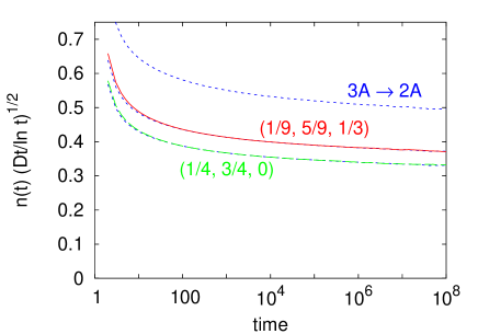
Figure 5: The density $n(t)$ for the $3A\to 2A$ reaction, as well as for two mixed reactions as labeled (see text). Also plotted is the $3A\to 2A$ data scaled by factors of $3/4$ and $2/3$, which overlays the mixed reaction data as predicted by the field rescaling transformation.

V Smoluchowski Theory

Smoluchowski theory is a mean-field theory based on the correlation function, or conditional density, as compared to rate equations which are based on the density. Interestingly, Smoluchowski theory is capable of capturing much of the behavior of the $d<d_{c}$, fluctuation-dominated systems missed by the rate equations: for the $A+A\to(\emptyset,A)$ reactions it gives the correct upper critical dimension $d_{c}=2$, correct decay exponents above and below $d_{c}$, and even exhibits logarithmic corrections at the critical dimension. However, the approach does involve an uncontrolled approximation and is known to have limitations. For example, the Smoluchowski density decay amplitude in $d=1$ differs from exact solutions by a factor of $\pi/2$ Torney and McConnell (1983), and in multi-species reactions even the exponents can be wrong Howard (1996).

However, Smoluchowski theory gives, surprisingly, the correct amplitude for the $kA\to\ell A$ reaction at the upper critical dimension $d_{c}=2/(k-1)$ for $k=2$ and $3$, as we demonstrate in this section. We first present the basic approach for two-particle reactions $A+A\to(\emptyset,A)$ in some detail, as this is necessary for getting the various factors correct and for generalizing to the three-particle case.

V.1 $A+A\to(\emptyset,A)$ reaction in $d=2$

A coordinate system origin is attached to one of particles. The motion of the other particles in this coordinate system remains diffusive with an effective diffusion constant $\tilde{D}=2D$, as can be straightforwardly verified from the continuum Green’s functions for the diffusion equation. The Smoluchowski theory is then built on the conditional density $n(r,t)$, where $r$ is the radial distance from the particle at the origin. First, $n(r,t)$ is assumed to evolve via the diffusion equation,

$$\frac{\partial}{\partial t}n(r,t)=\tilde{D}\nabla^{2}n(r,t),$$ (21)

subject to boundary conditions $n(R,t)=0$, where $R$ is the radius of the fixed particle, and $n(r\to\infty,t)=n_{\infty}$, and initial condition $n(r,0)=n_{\infty}$. The solution of eq. (21) is used to determine the particle current ${\bf j}=-\tilde{D}\nabla n(r,t)$, which in turn gives the flux of particles toward the origin,

$$F=-\oint dS\,\hat{n}\cdot{\bf j}|_{r=R}=-S_{d}\tilde{D}\left(\frac{\partial n}{\partial r}\right)_{r=R}$$ (22)

where $S_{d}$ is the surface area of the $d$-dimensional unit hypersphere. The flux $F$ then determines the decay rate of the probability $p$ that the particle at the origin has not been visited by another particle, i.e., $\dot{p}=-Fp$.

This can be turned into an equation for the density decay by considering each particle in turn to be the fixed particle. Since each meeting of particles involves two particles and removes $2-\ell$ particles, the density will decay according to

$$\frac{dn}{dt}=-\frac{2-\ell}{2}Fn.$$ (23)

To close these equations, $n_{\infty}$ is taken to be $n(t)$. This amounts to a quasistatic approximation, since the time-dependence of the large $r$ boundary condition is neglected when solving eq. (21). The second approximation in Smoluchowski theory is that the exterior particles are treated as only diffusing, and reactions are re-incorporated in a mean-field way via the decaying density used as the large $r$ boundary condition.

Now consider the case of $d=2$. For times $t\gg R^{2}/D$ the solution to eq. (21) in the region $R\leq r\ll(Dt)^{1/2}$ is given by Carslaw and Jaeger (1953)

$$n(r,t)=\frac{2n_{\infty}}{\ln t}\ln(r/R).$$ (24)

The resulting flux is $F=4\pi n_{\infty}\tilde{D}/\ln t$. Taking $n_{\infty}\to n(t)$ gives, via eq. (23),

$$\frac{dn}{dt}=-\frac{4\pi(2-\ell)D}{\ln t}n^{2}.$$ (25)

where we have substituted back the lab frame diffusion constant. This has the form of the mean-field rate equation with a time-dependent rate constant that decays as $1/\ln t$. Eq. (25) results in an asymptotic density of the form $n\sim A\ln t/(Dt)$, with the amplitude matching the RG value, eq. (2), and the exact solution Bramson and Griffeath (1980). We believe this to be the first demonstration that Smoluchowski theory predicts the correct amplitude at the upper critical dimension.

Finally, we comment on the case where the particles are not circular. The boundary condition for the conditional density remains $n({\bf r},t)=0$ for points ${\bf r}$ on the particle surface. While we are unaware of a formal exact solution to eq. (21) for this case, we appeal to the quasistatic approach presented in Krapivsky (1994). The conditional density is assumed to obey Laplace’s equation in the region exterior to the particle at the origin but within the diffusion radius $R_{D}=\alpha(Dt)^{1/2}$, where $\alpha$ is an arbitrary constant. The outer boundary condition is taken to be $n(R_{D},t)=n_{\infty}$. For a circular particle, this approach reproduces the known solution, eq. (24). For a non-circular particle, it is straightforward to demonstrate via separation of variables that the solution is unmodified apart from an additive constant (with respect to $r$) and additional subasymptotic terms that decay as powers of $t$. This suggests the asymptotic Smoluchowski flux and subsequent density are universal with respect to particle shape.

V.2 $3A\to\ell A$ reaction in $d=1$

Two approaches have been used to extend Smoluchowski theory to the case of three-particle, one species reactions in one dimension. Both approaches yielded densities with the logarithmic correction to the rate equation result.

Krapivsky’s method Krapivsky (1994) is to consider a fixed particle and then construct pseudo-particles in a $d=2$ plane out of every possible pair of particles, i.e. real particles at points $x_{1}$ and $x_{2}$ in the one-dimensional system would contribute a pseudo-particle at $(x_{1},x_{2})$. In this viewpoint a three-particle reaction corresponds to a pseudo-particle meeting the fixed particle at the origin. Krapivsky proposes to approximate the pseudo-particle dynamics as independently diffusing particles, even though their motion is correlated, with the net result that the problem reduces to the $d=2$ two-particle reaction. The only difference is that the $n_{\infty}$ represents the pseudo-particle density, which is given by $n(t)^{2}$, where $n(t)$ is the $d=1$ particle density. The corresponding equation becomes $\partial_{t}n\sim-Dn^{3}/\ln t$, which exhibits the expected $n\sim\sqrt{\ln t/Dt}$ behavior.

The second approach, due to Oshanin, Stemmer, Luding, and Blumen (OSLB) Oshanin et al. (1995), is based on the three-point correlation function, which due to translational invariance is a function of two distances. OSLB show that this correlation function, in the absence of reactions, satisfies an anisotropic two-dimensional diffusion equation in the plane defined by the two arguments. Reactions are then incorporated into this pseudo-two-dimensional system via the Smoluchowski approach.

We argue that at the level of the Smoluchowski approximation these two approaches are the same. The three-point correlation function viewed in the 2D plane is, in fact, the average of Krapivsky’s pseudoparticles over stochastic initial conditions and diffusion hops. Such an averaging is implicit in the Krapivsky method in going to the pseudoparticle diffusion equation, so at this point the two approaches should be formally identical. We now proceed to solve this system.

First, we observe that Krapivsky’s pseudo-particles indeed satisfy the same anisotropic diffusion equation as the OSLB. Let $y_{i}(t)\equiv x_{i}(t)-x_{i}(0)$ represent the displacement at time $t$ of the $i$th particle from its initial position. The single particle Green’s function is $G(y,t)\propto e^{-y^{2}/(4Dt)}$, where we neglect normalization factors for clarity. We attach a coordinate origin to particle $i=0$ by introducing the variables $u_{i}=y_{i}-y_{0}$. Now consider a pair of exterior, $i\neq 0$ particles, which we take to be $i=1$ and $2$. The combined Green’s function in the Smoluchowski frame is given by

$$G_{2}(u_{1},u_{2},t) =\int dy_{0}\,G(y_{0},t)\,G(y_{1},t)\,G(y_{2},t)$$ (26)

$$\propto\exp\Bigl{[}-\frac{1}{6Dt}(u_{1}^{2}+u_{2}^{2}-u_{1}u_{2})\Bigr{]}$$

The $u_{1}u_{2}$ cross-term indicates anisotropic diffusion, which may be diagonalized by a $\pi/4$ rotation. Taking $v_{1}=(u_{1}+u_{2})/\sqrt{2}$ and $v_{2}=(u_{1}-u_{2})/\sqrt{2}$ gives

$$G_{2}(v_{1},v_{2},t)\propto\exp\Bigl{[}-\frac{v_{1}^{2}}{12Dt}-\frac{v_{2}^{2}}{4Dt}\Bigr{]}$$ (27)

By comparison with the single-particle Green’s function we find that in the $v_{1}$ direction the effective diffusion constant is $D_{1}=3D$, while in the $v_{2}$ direction $D_{2}=D$. This can be understood by noting that changes in $y_{0}$, that is, the motion of the particle at the origin, affects $u_{1}$ and $u_{2}$ identically, thus enhancing the motion of their sum relative to their difference.

To make the Smoluchowski approximation one then solves this anisotropic diffusion equation in the $v$ plane. We first rescale $\tilde{v}_{1}=v_{1}/\sqrt{3}$ and $\tilde{v}_{2}=v_{2}$ to get isotropic diffusion. The rescaling affects the shape of the interior boundary condition, but as argued above, this should not affect the position-dependent part of the density at distances small compared to $(Dt)^{1/2}$. Mapping back to the $v$ plane we find

$$n(v_{1},v_{2},t)\sim(n_{\infty}/\ln t)\ln(v_{1}^{2}/3+v_{2}^{2})+\mbox{const.}$$ (28)

in the region $v_{1},v_{2}\ll(Dt)^{1/2}$. The particle current in the pseudo-particle plane is then

$${\bf j} =-\left(3D\frac{\partial}{\partial v_{1}}+D\frac{\partial}{\partial v_{2}}\right)n(v_{1},v_{2},t)$$ (29)

$$=-\frac{2n_{\infty}D}{(v_{1}^{2}/3+v_{2}^{2})\ln t}(v_{1}\hat{v}_{1}+v_{2}\hat{v}_{2})$$ (30)

Interestingly, current is directed radially inward despite the anisotropy. The flux through a circular region encompassing the fixed particle is

$$F=\frac{2n_{\infty}D}{\ln t}\int_{0}^{2\pi}\frac{d\theta}{\frac{1}{3}\cos^{2}\theta+\sin^{2}\theta}=\frac{4\sqrt{3}\pi n_{\infty}D}{\ln t}$$ (31)

Now we generate an equation for the density $n(t)$ of our one-dimensional system. As before, we generate an equation for the density by considering each particle in turn to be fixed at the origin. This brings a factor of $(3-\ell)/3$ since each reaction removes $3-\ell$ particles and is counted three times. Furthermore, since each particle pair contributes two pseudo-particles, i.e., at $(x_{1},x_{2})$ and $(x_{2},x_{1})$, the flux of pseudoparticles to the origin double counts the reactions with the particle at the origin. The net result is

$$\frac{dn}{dt}=-\frac{3-\ell}{6}Fn=-\frac{2\sqrt{3}(3-\ell)\pi D}{3\ln t}n^{3}$$ (32)

where in the last step we have taken $n_{\infty}=n(t)^{2}$. As with the $A+A\to(\emptyset,A)$ reactions in $d=2$, this has the rate equation form with a $1/\ln t$ reaction rate. The resulting density is of the expected form $n\sim A\sqrt{\ln t/(Dt)}$, with the amplitude $A$ matching the RG result, eq. (2). However, we note that the universal leading corrections predicted by the RG are absent, i.e., according Smoluchowski theory $B_{3,\ell}=0$.

Our result for the Smoluchowski amplitudes differ quantitatively from Krapivsky Krapivsky (1994), who did not consider the anisotropic nature of the diffusion, and from OSLB Oshanin et al. (1995), who omitted the factor of three due to the number of particles removed in $3A\to\emptyset$ and the factor of $1/2$ due to double-counting the rate of reactions at the origin. With these factors included, the OSLB result becomes equivalent to eq. (32).

VI Summary

The present work was motivated by the apparent discrepancy between the simulations and RG predictions. This discrepancy was resolved by demonstrating that the densities measured by simulation, which appear to be asymptotic in plots such as Fig. 1, are in fact consistent with the RG predictions of significant subasymptotic contributions, as demonstrated in Figs. 2, 3, and 4. Unfortunately, we also conclude that a more precise test of the RG predictions by direct comparison to simulations is not possible, owing to the slow decay of the higher order terms in a $1/\sqrt{\ln t}$ expansion.

In view of this, it is significant that exact solutions are available for the $A+A\to(\emptyset,A)$ reactions in $d=d_{c}=2$, which do provide a strong test of the RG results. It is also significant that relations predicted via the field rescaling transformation between pure and mixed reactions can be tested by simulations and appear to hold with no slow transients. Given that these $k=2$ amplitudes are correct, that the field rescaling transformation predictions hold, that there is no discrepancy with simulation in the pure $3A\to\ell A$ reactions, and that in principle no approximation is made in the RG treatment, it seems reasonable to believe the RG amplitudes reported here are exact results.

As is the usual benefit of an RG calculation, these amplitudes are also demonstrated to be universal, thus the predictions are subject to testing by future exact solutions for any particular realization of the dynamics.

A final result of our study is the demonstration that there is a single Smoluchowski theory for the $3A\to\ell A$ reaction in one dimension, and that this approximate theory indeed yields the exact asymptotic density. Since this property is shared by the $A+A\to(\emptyset,A)$ reaction in $d=2$, it appears to be a general feature of Smoluchowski theory that it succeeds quantitatively at the upper critical dimension. It may be possible to find an underlying explanation for this property, which would be an interesting direction for future work.